On application of empirical mode decomposition for turbulence analysis in open-channel flows

Abstract

Large-scale coherent structures are key elements of open-channel flow turbulence, quantification of which remains elusive. In this work, we use empirical mode decomposition (EMD) to break down a velocity time series into different modes, denoted as “intrinsic mode functions” (IMFs). Analysis of velocity auto- and co-spectra indicates that large-scale (LSMs) and very large-scale (VLSMs) fluid motions are sufficiently represented by particular groups of IMFs. A correlation between LSMs and VLSMs, identified by the EMD analysis, was found to generate 7% of the Reynolds shear stresses. However, the EMD analysis of surrogate velocity signals with randomized spectral phases demonstrated that the revealed correlation is actually an artefact of the EMD approach and should not be interpreted physically.

Keywords:

• Coherent structures
• empirical mode decomposition
• open-channel flow
• turbulence
• velocity spectra

1 Introduction

Turbulence in open-channel flows (OCFs) involves various types of eddies and coherent structures that scale with the viscous length, roughness height, distance z from the wall, and flow depth H, including: (1) near-bed streaks in smooth-bed OCFs (e.g. Nezu & Nakagawa, 1993) or wake eddies due to roughness elements in rough-bed OCFs (e.g. Nikora, 2008); (2) hairpin vortices (scaled with z, e.g. Adrian & Marusic, 2012; Nezu & Nakagawa, 1993); (3) large-scale motions (LSMs, e.g. hairpin packets) with a length scale of ≈ 2H to ≈ 4H and (4) very large-scale motions (VLSMs), or superstructures, with lengths up to 50H or even longer (e.g. Adrian & Marusic, 2012; Cameron et al., 2017; Duan et al., 2020, 2021; Peruzzi et al., 2020; Zampiron, Cameron, et al., 2020). Among them, LSMs and VLSMs are the main contributors to the turbulent energy and momentum fluxes (Cameron et al., 2020; Duan et al., 2020; Zampiron, Cameron, et al., 2020), and therefore a better understanding of large-scale turbulence is required. This enhanced knowledge may lead to improved modelling, prediction and perhaps control of flow drag (Zampiron, Cameron, et al., 2020), as well as to novel models of sediment transport, diffusion of substances and flow–biota interactions.

The contributions of LSMs and VLSMs to turbulence quantities (e.g. turbulent kinetic energy and momentum fluxes) can be estimated using different methods. The most common and simplest approach involves an intuitively defined separation wavelength (or wavenumber) that divides LSMs and VLSMs in velocity spectra (e.g. Duan et al., 2020; Guala et al., 2006; Hutchins & Marusic, 2007), thereby allowing the detection of LSM and VLSM contributions to velocity signals and turbulence statistics. However, despite the attractiveness of this approach, a separation wavelength does not represent an actual border between turbulent structures, which are likely to overlap in the spectral space over a range of wavenumbers. In an attempt to overcome this limitation, empirical mode decomposition (EMD, Huang et al., 1998) can be used to separate velocity signals into modes, known as “intrinsic mode functions” (IMFs). Indeed, unlike the sinusoidal Fourier components, each of these modes covers a range of wavenumbers, thereby allowing a coexistence of EMD-based modes in the spectral domain. Another velocity decomposition method is the proper orthogonal decomposition (POD, e.g. Holmes et al., 2012; Zampiron, Cameron, et al., 2020), which divides a velocity field into fully orthogonal (i.e. uncorrelated) modes. However, since the POD modes and the Fourier modes coincide for a 1D stationary velocity signal (which is a typical case of one-point measurements such as those used in this study), POD is not explored further.

EMD is gradually becoming a common tool for studying turbulent flows (e.g. Agostini & Leschziner, 2014, 2019; Franca & Lemmin, 2015; Peruzzi et al., 2021), and it is therefore beneficial to assess its advantages and limitations, particularly in relation to LSMs and VLSMs. The analysis presented in this work undertakes such an assessment using long-duration (8 h) acoustic-Doppler-velocimetry (ADV) records in rough-bed OCF. First, we will briefly introduce the experimental methodology (Section 2) and the EMD algorithm (Section 3). In Section 4, the results are outlined, including: examples of EMD modes (Section 4.1); the assessment of the contributions of LSMs and VLSMs to velocity auto- and co-spectra, and to turbulent stresses (Sections 4.2 and 4.3); and the analysis of surrogate velocity signals generated through phase randomization in the Fourier space, to evaluate the potential interrelations between LSMs and VLSMs identified by EMD (Section 4.4). Finally, the main outcomes of this work are summarized and discussed in Section 5.

2 Velocity measurements

ADV (Vectrino, Nortek) measurements were performed in the RS flume of the University of Aberdeen (0.4 m wide and 10.75 m long, e.g. Zampiron, Cameron, et al., 2020). The three velocity components were measured continuously for 8 h with a sampling frequency of 100 Hz at a relative elevation of z/H = 0.3 from the mean channel bed (z is wall-normal coordinate and H = 80.2 mm is mean flow depth). The measurements were located at 125H from the channel entrance, ensuring a good degree of flow development and the emergence of LSMs and VLSMs (Zampiron et al., 2023). The flow was steady and uniform for the total duration of the measurements. The bed of the channel was entirely covered by micro hooks (Pressogrip®) with a height of ≈1 mm, which ensured fully rough-bed flow conditions (Zampiron, Nikora, et al., 2020). The aspect ratio (i.e. width-to-depth) of 5 suggests quasi-two-dimensional flow conditions at the centre of the channel where measurements were made (e.g. Nezu & Nakagawa, 1993). Hydraulic parameters are listed in Table 1. The 8-hour velocity time series are provided in the online Supplemental Material. Further details on the measurements can be found in Zampiron et al. (2023).

Table 1 Flow conditions for the ADV measurements

H (mm)	Sb (%)	$u_{\ast }$ (m s^−1)	U (m s^−1)	Re (−)	F (−)	B/H (−)	H/Δ (−)	H^+ (−)	Δ^+ (−)
80.2	0.106	0.029	0.378	30,300	0.43	5.0	72.9	2320	32

Note: Experimental and analysis parameters: H is mean flow depth; S_b is bed slope; $u_{\ast }=\sqrt{gH{S}_b}$ is shear velocity, g is gravity acceleration; U = Q/(BH) is bulk flow velocity, Q is flowrate, B is channel width; ${\mathsf{R}}_{\mathsf{e}}=UH/\nu$ is bulk Reynolds number, ν is fluid kinematic viscosity; $\mathsf{F}=U/\sqrt{gH}$ is Froude number; B/H is flow aspect ratio; H/Δ is relative submergence, Δ is roughness height; $H^{+}=u_{\ast }H/\nu$ is friction Reynolds number, superscript + denotes normalization by the viscous length $\nu /u_{\ast }$; and ${\Delta }^{+}=u_{\ast }\Delta /\nu$ is roughness Reynolds number.

3 Empirical mode decomposition (EMD) algorithm

EMD is used to decompose a generic time series θ(t) (which can be stationary or not, t is time) into a set of IMFs. The IMFs exhibit a dominant frequency that gradually decreases as the IMF order (m) increases from m = 1 to M, where M represents the total number of IMFs. An IMF must satisfy two conditions (Huang et al., 1998): (i) the count of extrema and zero-crossings must either be equal or differ by at most one; and (ii) the local mean values of the upper and lower envelopes must be zero or, in other words, the two envelopes must be symmetric about zero. It is important to note that IMFs may not necessarily be orthogonal and thus can exhibit some degree of correlation. Our implementation of EMD stems from Huang et al. (1998) and follows a sifting process to extract iteratively the mth IMF of a signal θ ($IM{F}_{\theta }^m$).

The IMF order is initially set to m = 1. At the first iteration (n = 1, where n is iteration number), a provisional signal h is defined for the mth IMF as: (1) $\{\begin{array}{ll}{h}_{n=1}^m=\theta & \text{for }m=1\\ h_{n=1}^m=\theta -\sum _{\alpha =1}^{m-1}IM{F}_{\theta }^{\alpha }& \text{for}m>1\end{array}$(1) where α is a summation index. A new provisional signal $h_{n+1}^m$ is computed for the next iteration n + 1 as: (2) $h_{n+1}^m=h_n^m-e_n^m$(2) where $e_n^m$ is the mean of the envelopes of $h_n^m$. Upper and lower envelopes are computed by fitting a cubic spline through the maxima and minima of $h_n^m$, respectively. However, this interpolation scheme is inefficient at the start and the end of the times series, resulting in unrealistic values that, through multiple iterations, can propagate throughout the signal. This issue was mitigated by the repetition of the extrema at the start and end of the signal (Huang et al., 1998).

Equation (2) is repeated iteratively, with n = n + 1 at each new iteration, until the following condition is satisfied: (3) $\sqrt{\frac{\sum _t{\left(h_n^m-h_{n+1}^m\right)}^2}{\sum _t{\left(h_n^m\right)}^2}}\le ϵ$(3) where ε is a threshold value assumed ε = 0.1 (Huang et al., 1998). Once the algorithm reaches convergence, the mth IMF of the signal θ is obtained as $IM{F}_{\theta }^m=h_{n+1}^m$ and we may move to the (m + 1)th IMF. The process is repeated from Eq. (1) and continues until no further extrema can be detected in $h_{n=1}^{m+1}$, thus setting the total number of IMFs to M = m. The remaining monotonic signal $h_{n=1}^{m+1}$ represents the residual r_θ. In the case of stationary data, r_θ is equal to the time-averaged value $\overline{\theta }$ of the signal θ (overbar indicates time averaging).

Once all M IMFs have been obtained, EMD-filtered signals 〈θ〉 can be computed as: (4) $〈\theta 〉\left(t\right)=\sum _{m=m_1}^{m_2}IM{F}_{\theta }^m\left(t\right)$(4) where m₁ and m₂ are chosen summation limits. The original signal θ is reconstructed as: (5) $\theta \left(t\right)=\sum _{m=1}^{M}IM{F}_{\theta }^m\left(t\right)+r_{\theta }\left(t\right)$(5) A comprehensive review of the EMD approach and application examples are given in Huang and Shen (2014).

4 Results

In this work, we employ EMD to quantify the contributions of LSMs and VLSMs to velocity spectra and to turbulent stresses $\overline{u^{\mathrm{\prime }}{u}^{\mathrm{\prime }}}$, $\overline{w^{\mathrm{\prime }}{w}^{\mathrm{\prime }}}$ and $\overline{u^{\mathrm{\prime }}{w}^{\mathrm{\prime }}}$, where u^′ and w^′ are turbulent fluctuations of the streamwise (u) and vertical (w) velocity components, respectively, i.e. $u^{\mathrm{\prime }}=u-\overline{u}$ and $w^{\mathrm{\prime }}=w-\overline{w}$. Then, the obtained estimates are compared with those computed using the LSM-VLSM separation wavelength (Section 1) applied to the conventional velocity spectra. Considering that the length of both LSMs and VLSMs exceeds the flow depth H, we focus on streamwise wavelengths larger than H. The components in the streamwise (x), spanwise (y) and wall-normal (z) directions of the velocity vector are denoted as u, v and w, respectively.

4.1 Decomposition of velocity signals

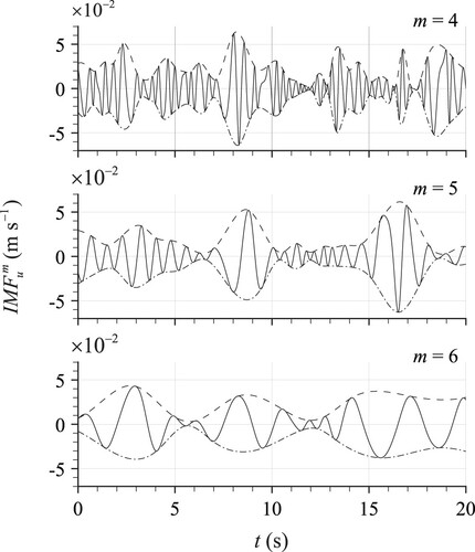
EMD (Section 3) was used to decompose the 8-h record of each velocity component (Section 2) into M_u = 13 IMFs for u, and M_v = M_w = 12 IMFs for v and w. Note that the number of IMFs is not universal and may depend on the specifics of the EMD algorithm (e.g. convergence criteria). In Fig. 1, we show 20 s long samples for a subset of IMFs of the streamwise velocity u ($IM{F}_u^m$, with m = 4 to 6) together with their envelope curves. IMFs belonging to the other velocity components and/or of different order are qualitatively similar. As expected, the dominant frequency of the IMFs decreases with increase in m, while upper and lower envelopes exhibit a good level of symmetry (conditions of Huang et al., 1998).

Figure 1 Selected IMFs (m = 4,5,6) of the streamwise velocity $IM{F}_u^m$ (solid lines). Dashed and dash-dotted lines represent upper and lower envelopes, respectively

4.2 LSM and VLSM contributions to velocity auto- and co-spectra

In this section, EMD is used to assess the contributions of LSMs and VLSMs to the pre-multiplied auto-spectra of the streamwise k_xS_uu(k_x) and vertical k_xS_ww(k_x) velocity components, and to the pre-multiplied co-spectrum k_xC_uw(k_x) of u and w, where k_x = 2π / λ_x and λ_x are streamwise wavenumber and wavelength, respectively. In our estimates we assume the validity of Taylor’s “frozen turbulence” hypothesis for OCFs, that gives ${\lambda }_x=\overline{u}/f$ where f is frequency (e.g. Nikora & Goring, 2000). Spectra were computed for 2800 subsections 20.48 s long with a 50% overlap, which were then ensemble averaged. Pre-multiplied velocity spectra are particularly convenient for studying large-scale flow structures as they show energy distributions of the velocity fluctuations as a function of the spectral wavelength (unlike conventional power spectra that show energy density distributions). Auto-spectrum S_vv exhibits low energy within the VLSM wavelength range and therefore is not considered in this paper.

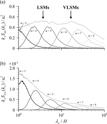
In Fig. 2, we show k_xS_uu(k_x) and k_xS_ww(k_x) of the original signals (dotted lines) together with the contributions from the IMFs. The spectrum of the original streamwise velocity signal (Fig. 2a) reveals two distinct “hills” at wavelengths of ≈3.5H and ≈17H, reflecting the presence of LSMs and VLSMs, respectively (e.g. Cameron et al., 2017; Kim & Adrian, 1999; Zampiron, Cameron, et al., 2020). As expected from Fig. 1, the dominant wavelength (i.e. corresponding to the spectral “hill”) in the IMF spectra increases with m. The low-frequency IMFs 9 ≤ m ≤ 13 contain a small amount of energy at wavelengths exceeding the VLSM range (where our spectra are not resolved due to the limited size of the time subsections) and therefore are not visible.

Figure 2 Pre-multiplied auto-spectra of the mth IMF of the (a) streamwise u and (b) vertical w velocity components as functions of the normalized streamwise wavelength λ_x/H. Dotted lines show the spectra of the original velocity signals

In Fig. 3, the original auto- and co-spectra are compared to the contributions attributed to LSMs and VLSMs estimated using EMD. Considering that a zero-mean (i.e. fluctuating) velocity time series can be expressed as the sum of its IMFs (Eq. 5), the auto-spectra of the streamwise (S_uu) and vertical (S_ww) velocity components can be expressed as (e.g. Bendat & Piersol, 2010, page 126): (6) $\begin{array}{rl}& S_{uu}=\underset{\mathrm{L}\mathrm{S}\mathrm{M}}{\underbrace{S_{{〈u〉}_{\mathrm{L}\mathrm{S}\mathrm{M}}{〈u〉}_{\mathrm{L}\mathrm{S}\mathrm{M}}}}}+\underset{\mathrm{V}\mathrm{L}\mathrm{S}\mathrm{M}}{\underbrace{S_{{〈u〉}_{\mathrm{V}\mathrm{L}\mathrm{S}\mathrm{M}}{〈u〉}_{\mathrm{V}\mathrm{L}\mathrm{S}\mathrm{M}}}}}+\underset{\mathrm{L}\mathrm{S}\mathrm{M}-\mathrm{V}\mathrm{L}\mathrm{S}\mathrm{M}}{\underbrace{2C_{{〈u〉}_{\mathrm{L}\mathrm{S}\mathrm{M}}{〈u〉}_{\mathrm{V}\mathrm{L}\mathrm{S}\mathrm{M}}}}}+{\Phi }_{uu}\end{array}$(6) (7) $\begin{array}{rl}& S_{ww}=\underset{\mathrm{L}\mathrm{S}\mathrm{M}}{\underbrace{S_{{〈w〉}_{\mathrm{L}\mathrm{S}\mathrm{M}}{〈w〉}_{\mathrm{L}\mathrm{S}\mathrm{M}}}}}+\underset{\mathrm{V}\mathrm{L}\mathrm{S}\mathrm{M}}{\underbrace{S_{{〈w〉}_{\mathrm{V}\mathrm{L}\mathrm{S}\mathrm{M}}{〈w〉}_{\mathrm{V}\mathrm{L}\mathrm{S}\mathrm{M}}}}}+\underset{\mathrm{L}\mathrm{S}\mathrm{M}-\mathrm{V}\mathrm{L}\mathrm{S}\mathrm{M}}{\underbrace{2C_{{〈w〉}_{\mathrm{L}\mathrm{S}\mathrm{M}}{〈w〉}_{\mathrm{V}\mathrm{L}\mathrm{S}\mathrm{M}}}}}+{\Phi }_{ww}\end{array}$(7) Similarly, for the velocity co-spectrum (C_uw) we have: (8) $\begin{array}{rl}{C}_{uw}& =\underset{\mathrm{L}\mathrm{S}\mathrm{M}}{\underbrace{C_{{〈u〉}_{\mathrm{L}\mathrm{S}\mathrm{M}}{〈w〉}_{\mathrm{L}\mathrm{S}\mathrm{M}}}}}+\underset{\mathrm{V}\mathrm{L}\mathrm{S}\mathrm{M}}{\underbrace{C_{{〈u〉}_{\mathrm{V}\mathrm{L}\mathrm{S}\mathrm{M}}{〈w〉}_{\mathrm{V}\mathrm{L}\mathrm{S}\mathrm{M}}}}}\\ & +\underset{\mathrm{L}\mathrm{S}\mathrm{M}-\mathrm{V}\mathrm{L}\mathrm{S}\mathrm{M}}{\underbrace{C_{{〈u〉}_{\mathrm{L}\mathrm{S}\mathrm{M}}{〈w〉}_{\mathrm{V}\mathrm{L}\mathrm{S}\mathrm{M}}}+C_{{〈u〉}_{\mathrm{V}\mathrm{L}\mathrm{S}\mathrm{M}}{〈w〉}_{\mathrm{L}\mathrm{S}\mathrm{M}}}}}+{\Phi }_{uw}\end{array}$(8) The parts of the jth velocity component (u_j) representing LSMs (〈u_j〉_LSM) and VLSMs (〈u_j〉_VLSM) are reconstructed as the sums of different IMFs using Eq. (4). The remaining energy of S_uu, S_ww and C_uw, not associated with LSMs, VLSMs, or their combination, is represented by the terms $\Phi$_uu, $\Phi$_ww and $\Phi$_uw, respectively (shown as grey areas in Fig. 3).

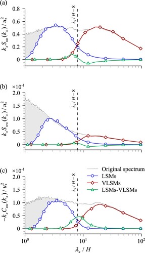
Figure 3 EMD contributions (Eqs 6–8) to pre-multiplied (a) streamwise velocity auto-spectrum, (b) vertical velocity auto-spectrum, and (c) uw co-spectrum. Vertical dashed lines show the separation wavelength λ_x / H = 8 used in Section 4.3. Grey areas show energy that is not associated with LSMs, VLSMs or their combination ($\Phi$_uu, $\Phi$_ww and $\Phi$_uw in Eqs 6–8, respectively)

To define the LSM and VLSM signals, appropriate summation limits (m₁ and m₂, defined in Eq. 4) are chosen based on seeking a good visual agreement between the shape and peaks in the original spectra, and the LSM and VLSM spectra computed from the constructed signals 〈u_j〉_LSM and 〈u_j〉_VLSM (Fig. 3), i.e. $〈u{〉}_{\mathrm{L}\mathrm{S}\mathrm{M}}={\sum }_{m=4}^{5}IM{F}_u^m$, $〈w{〉}_{\mathrm{L}\mathrm{S}\mathrm{M}}={\sum }_{m=4}^{5}IM{F}_w^m$, $〈u{〉}_{\mathrm{V}\mathrm{L}\mathrm{S}\mathrm{M}}={\sum }_{m=6}^{M_u}IM{F}_u^m$ and $〈w{〉}_{\mathrm{V}\mathrm{L}\mathrm{S}\mathrm{M}}={\sum }_{m=6}^{M_w}IM{F}_w^m$. This approach is considered adequate due to the wide range of wavenumbers encompassed by each IMF (Fig. 2), which minimizes the subjectivity in selecting the IMFs. A similar approach was employed by Agostini and Leschziner (2014, 2019) when studying turbulence in closed-channel flows using two-dimensional EMD.

Similar to the streamwise auto-spectrum, velocity co-spectrum also exhibits a strong signature of VLSMs, indicating their sizeable contribution to turbulent momentum fluxes (or shear stresses). Figure 3 suggests that a noticeable contribution to S_uu and C_uw arises from a combined effect of LSMs and VLSMs (i.e. LSM–VLSM correlation, Eqs 6 and 8). The LSM-VLSM contribution to S_uu changes in sign with λ_x, while the contribution to -C_uw remains positive throughout. Considering the potential physical significance of this combined contribution, its origin will be explored in Section 4.4.

4.3 LSM and VLSM contributions to turbulent stresses

The portions of turbulent streamwise ($\overline{u^{\mathrm{\prime }}{u}^{\mathrm{\prime }}}$) and vertical ($\overline{w^{\mathrm{\prime }}{w}^{\mathrm{\prime }}}$) normal stresses, and of turbulent shear stresses ($\overline{u^{\mathrm{\prime }}{w}^{\mathrm{\prime }}}$) associated with LSMs and VLSMs are presented in Fig. 4. EMD estimates (Fig. 3) are compared to the separation wavelength method (introduced in Section 1). The separation wavelength is chosen at λ_x/H = 8, close to the intersection of the LSMs’ and VLSMs’ curves and the peak of the LSM-VLSM contribution to C_uw (Fig. 3c). The lower bound wavelength of the LSMs is set equal to the flow depth (λ_x/H = 1), where the LSM curve approximately reaches zero. Contributions to turbulent stresses are computed as the integrals of the respective velocity spectra, i.e. $〈\overline{u^{\mathrm{\prime }}{u}^{\mathrm{\prime }}}〉={\int }_0^{\mathrm{\infty }}{S}_{〈u〉〈u〉}\left(k_x\right)\text{d}{k}_x$, $〈\overline{w^{\mathrm{\prime }}{w}^{\mathrm{\prime }}}〉={\int }_0^{\mathrm{\infty }}{S}_{〈w〉〈w〉}\left(k_x\right)\text{d}{k}_x$ and $〈\overline{u^{\mathrm{\prime }}{w}^{\mathrm{\prime }}}〉={\int }_0^{\mathrm{\infty }}{C}_{〈u〉〈w〉}\left(k_x\right)\text{d}{k}_x$.

Figure 4 Estimated relative contribution of LSMs and VLSMs to streamwise ($\overline{u^{\mathrm{\prime }}{u}^{\mathrm{\prime }}}$) and vertical ($\overline{w^{\mathrm{\prime }}{w}^{\mathrm{\prime }}}$) normal stresses, and to shear stress ($\overline{u^{\mathrm{\prime }}{w}^{\mathrm{\prime }}}$) using EMD (empty bars) and a separation wavelength of λ_x/H = 8 (filled bars)

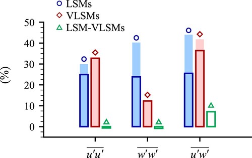
Using EMD, we estimate that ∼24–26% of normal and shear stresses are associated with LSMs, while VLSMs account for 33% of $\overline{u^{\mathrm{\prime }}{u}^{\mathrm{\prime }}}$, 12% of $\overline{w^{\mathrm{\prime }}{w}^{\mathrm{\prime }}}$ and 36% of $\overline{u^{\mathrm{\prime }}{w}^{\mathrm{\prime }}}$. The inter-scale (correlation) contribution LSM-VLSM (Eqs 6–8) is essentially negligible for $\overline{u^{\mathrm{\prime }}{u}^{\mathrm{\prime }}}$ and $\overline{w^{\mathrm{\prime }}{w}^{\mathrm{\prime }}}$ (due to the change of sign, Fig. 3a and b), whereas it accounts for 7% of the total shear stress $\overline{u^{\mathrm{\prime }}{w}^{\mathrm{\prime }}}$. Contributions of comparable magnitude have been earlier reported by Agostini and Leschziner (2019).

Using the separation wavelength method, the contributions from LSMs to velocity variances $\overline{u^{\mathrm{\prime }}{u}^{\mathrm{\prime }}}$ and $\overline{w^{\mathrm{\prime }}{w}^{\mathrm{\prime }}}$, and to velocity covariance $\overline{u^{\mathrm{\prime }}{w}^{\mathrm{\prime }}}$ are higher compared to the EMD estimates, primarily due to the minimum wavelength being set to λ_x/H = 1. The contributions of VLSMs to normal stresses closely match those obtained from EMD. However, a 42% VLSM contribution to $\overline{u^{\mathrm{\prime }}{w}^{\mathrm{\prime }}}$ exceeds the 36% from the EMD analysis. This discrepancy reflects the sharp transition between scales and the orthogonality of Fourier modes (i.e. LSM-VLSM cross-terms are expected to be zero due to the orthogonality). Cameron et al. (2020) and Duan et al. (2020) have reported contributions of VLSMs to $\overline{u^{\mathrm{\prime }}{u}^{\mathrm{\prime }}}$ of ∼40–50%, and to $\overline{u^{\mathrm{\prime }}{w}^{\mathrm{\prime }}}$ of ∼30–60%.

The above EMD results, together with those presented in Section 4.2, suggest the potential importance of the LSM-VLSM term as it may relate to interactions of LSMs and VLSMs and energy exchanges between them. The validity of such an interpretation is assessed in the next section.

4.4 The nature of LSM-VLSM correlation within the EMD approach

The nature of the correlated contribution from LSMs and VLSMs can be studied by randomizing the spectral phases of the velocity signals (Prichard & Theiler, 1994). Using phase randomization, we can generate surrogate signals (denoted by tilde) that preserve LSM and VLSM energy contributions to S_uu, S_ww and C_uw (Eqs 6–8), while suppressing any cross-correlation between LSMs and VLSMs. Only the co-spectrum C_uw will be considered, for brevity, but a qualitatively similar behaviour is also observed for the auto-spectra S_uu and S_ww.

The Fourier transform of a generic signal θ is $\Theta =A\left(f\right)e^{i\varphi \left(f\right)}$, where A is the amplitude, i is the imaginary unit and ϕ is the phase angle. The phase of $\Theta$ can be randomized as $\tilde{\Theta }=A\left(f\right)e^{i\left[\varphi \right(f)+\phi (f\left)\right]}$, where φ obeys a uniform random distribution within [0, 2π]. Thus, the phase-randomized signal $\tilde{\theta }$ can be computed as the inverse Fourier transform of $\tilde{\Theta }$. Following these steps, any velocity signal involved in Eqs (6–8) is phase-randomized. Using the same φ for different velocity components preserves the cross-correlation between them, which is otherwise destroyed (Prichard & Theiler, 1994).

In Fig. 5a, we show co-spectra of phase-randomized EMD velocity signals ${\widetilde{〈u_j〉}}_{\mathrm{L}\mathrm{S}\mathrm{M}}$ and ${\widetilde{〈u_j〉}}_{\mathrm{V}\mathrm{L}\mathrm{S}\mathrm{M}}$, with phase randomization applied after the EMD of the original velocity record. In this case, the cross-correlation between u and w is preserved, while the cross-correlation (if any) between LSM and VLSM signals is eliminated by phase randomization. This result is achieved by using a random phase angle φ that is the same for u and w, but different for their LSM and VLSM parts. The LSM and VLSM contributions in Fig. 5a are the same as in Fig. 3c, while the LSM-VLSM correlation term is suppressed by phase-randomization. As a result, the sum of the LSM and VLSM contributions (dashed line) deviates from the spectra of the original signal.

Figure 5 Co-spectra of (a) phase-randomized EMD signals ${\widetilde{〈u_j〉}}_{\mathrm{L}\mathrm{S}\mathrm{M}}$ and ${\widetilde{〈u_j〉}}_{\mathrm{V}\mathrm{L}\mathrm{S}\mathrm{M}}$; and of (b) signal components ${〈\widetilde{〈u_j〉}〉}_{\mathrm{L}\mathrm{S}\mathrm{M}}$ and ${〈\widetilde{〈u_j〉}〉}_{\mathrm{V}\mathrm{L}\mathrm{S}\mathrm{M}}$ obtained by applying EMD to the phase-randomized velocity signal $\widetilde{〈u_j〉}$ (Section 4.4). Other lines, symbols and shadings are defined in Fig. 3

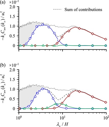
Then, EMD is applied a second time to a “surrogate” velocity signal $\widetilde{〈u_j〉}$ reconstructed as the sum of all its phase-randomized constituent signals, and thus free of any correlation between LSMs and VLSMs. Using the same m₁ and m₂ as in Section 4.2, ${〈\widetilde{〈u_j〉}〉}_{\mathrm{L}\mathrm{S}\mathrm{M}}$ and ${〈\widetilde{〈u_j〉}〉}_{\mathrm{V}\mathrm{L}\mathrm{S}\mathrm{M}}$ are obtained. Co-spectra of ${〈\widetilde{〈u_j〉}〉}_{\mathrm{L}\mathrm{S}\mathrm{M}}$ and ${〈\widetilde{〈u_j^{}〉}〉}_{\mathrm{V}\mathrm{L}\mathrm{S}\mathrm{M}}$ are shown in Fig. 5b. The co-spectrum computed as the sum of the different contributions (dashed line) is preserved by the EMD and therefore is the same as in Fig. 5a. However, we can observe the reappearance of the LSM-VLSM correlation term, which is balanced by a decrease in the LSM and VLSM co-spectra around λ_x/H ≈ 8 (Eq. 8).

This result explicitly demonstrates that the LSM-VLSM correlation observed in the EMD outputs (Sections 4.2 and 4.3) is actually introduced by the EMD procedure and does not reflect physical mechanism(s). While a certain degree of correlation between IMFs is expected due to the lack of orthogonality inherent in EMD, the energy content of such correlation should be small compared to the other contributions (Huang et al., 1998). However, in our case, the LSM-VLSM correlated contribution to the uw cospectrum is quite noticeable, highlighting a certain flaw of EMD when used to assess the effects of multi-scale fluid motions on turbulent fluxes of momentum. Consequently, any attempts to separate the contributions of different scales to $\overline{u^{\mathrm{\prime }}{w}^{\mathrm{\prime }}}$ using EMD and their physical interpretation should be approached with caution. Instead, the use of alternative approaches like the wavelength separation method or other decompositions procedures such as the “dynamic mode decomposition” (Schmid, 2010) may be more appropriate. On the other hand, the contribution of the LSM-VLSM correlation to autospectra is much less significant, indicating that EMD remains a valuable tool in this case, capable of extracting LSM and VLSM contribution to velocity spectra with a realistic overlap across a range of wavenumbers.

5 Conclusions

We used EMD to decompose velocity time-series into different modes (IMFs), which, unlike the Fourier components, can coexist over a range of spectral wavenumbers. Appropriately selected groups of IMFs were found to sufficiently represent the LSMs’ and VLSMs’ contributions to velocity times series, velocity auto-spectra and turbulent normal stresses (Section 4.2). The EMD analysis suggested that up to 7% of the turbulent shear stress may be due to the interactions (correlation) of LSMs and VLSMs (Section 4.3), with potentially important implications for scale-to-scale momentum exchanges and turbulence dynamics overall. However, non-zero values of the LSM-VLSM correlation terms in Eqs (5) and (6) could also reflect the lack of orthogonality of the IMFs. By randomizing the spectral phases of the velocity signals (Section 4.4), we demonstrated that the “correlated” contributions of LSMs and VLSMs to velocity spectra (Section 4.2) and turbulent stresses (Section 4.3) are an artefact of the EMD algorithm. In light of these considerations, any outcomes of the EMD analysis related to statistics across different velocity scales (e.g. in relation to Reynolds stresses and velocity co-spectra) should be treated with caution. On the other hand, our analysis suggests that EMD is an effective tool to isolate the signatures of LSMs and VLSMs on velocity signals and their contributions to auto-spectra and turbulent normal stresses for which the LSM-VLSM correlation term is negligible.

Notation

C(kx)	=	wavenumber velocity co-spectrum (m3 s−2 rad−1)
f	=	frequency (Hz)
h	=	provisional signal
H	=	mean flow depth (m)
IMFm	=	mth Intrinsic Mode Function
kx	=	streamwise wavenumber (rad m−1)
e	=	mean envelope
m	=	IMF order (−)
M	=	total number of IMFs (−)
r	=	residual
S(kx)	=	wavenumber velocity auto-spectrum (m3 s−2 rad−1)
t	=	time (s)
u	=	streamwise velocity component (m s−1)
v	=	spanwise velocity component (m s−1)
w	=	wall-normal velocity component (m s−1)
x	=	streamwise coordinate (−)
y	=	spanwise coordinate (−)
z	=	wall-normal coordinate (−)
ε	=	convergence threshold (−)
θ	=	generic time series
$\Theta$	=	Fourier transform of θ
λx	=	streamwise wavelength (m)
ϕ	=	phase angle (rad)
φ	=	random phase angle uniformly distributed within [0,2π] (rad)
$\Phi$	=	portion of velocity auto- or co-spectrum not associated to LSMs or VLSMs (m3 s−2 rad−1)
$\overline{\phantom{aa}}$	=	time averaging
〈  〉	=	EMD filtering
$\tilde{\phantom{0}}$	=	phase randomization

Acknowledgements

The authors wish to express their gratitude to Roy Gillanders for the help provided and to the School of Engineering of the University of Aberdeen for the support.

Supplemental data

Supplemental data for this article can be accessed https://doi.org/10.1080/00221686.2023.2241838.

Disclosure statement

No potential conflict of interest was reported by the authors.

Additional information

Funding

The study has been supported by the EPSRC/UK grants: “Bed friction in rough-bed free-surface flows: a theoretical framework, roughness regimes, and quantification” (EP/K041088/1) and “Secondary currents in turbulent flows over rough walls” (EP/V002414/1).

References

- Adrian, R. J., & Marusic, I. (2012). Coherent structures in flow over hydraulic engineering surfaces. Journal of Hydraulic Research, 50(5), 451–464. https://doi.org/10.1080/00221686.2012.729540
- Agostini, L., & Leschziner, M. A. (2014). On the influence of outer large-scale structures on near-wall turbulence in channel flow. Physics of Fluids, 26(7), 075107. https://doi.org/10.1063/1.4890745
- Agostini, L., & Leschziner, M. A. (2019). The connection between the spectrum of turbulent scales and the skin-friction statistics in channel flow at. Journal of Fluid Mechanics, 871, 22–51. https://doi.org/10.1017/jfm.2019.297
- Bendat, J. S., & Piersol, A. G. (2010). Random data: Analysis and measurement procedures (4th ed.). John Wiley & Sons, Inc.
- Cameron, S. M., Nikora, V. I., & Stewart, M. T. (2017). Very-large-scale motions in rough-bed open-channel flow. Journal of Fluid Mechanics, 814, 416–429. https://doi.org/10.1017/jfm.2017.24
- Cameron, S. M., Nikora, V. I., & Witz, M. J. (2020). Entrainment of sediment particles by very large-scale motions. Journal of Fluid Mechanics, 888, A7. https://doi.org/10.1017/jfm.2020.24
- Duan, Y. C., Chen, Q. G., Li, D. X., & Zhong, Q. (2020). Contributions of very large-scale motions to turbulence statistics in open channel flows. Journal of Fluid Mechanics, 892, A3. https://doi.org/10.1017/jfm.2020.174
- Duan, Y. C., Zhong, Q., Wang, G., Zhang, P., & Li, D. (2021). Contributions of different scales of turbulent motions to the mean wall-shear stress in open channel flows at low-to-moderate Reynolds numbers. Journal of Fluid Mechanics, 918, A40. https://doi.org/10.1017/jfm.2021.236
- Franca, M. J., & Lemmin, U. (2015). Detection and reconstruction of large-scale coherent flow structures in gravel-bed rivers. Earth Surface Processes and Landforms, 40(1), 93–104. https://doi.org/10.1002/esp.3626
- Guala, M., Hommema, S. E., & Adrian, R. J. (2006). Large-scale and very-large-scale motions in turbulent pipe flow. Journal of Fluid Mechanics, 554(-1), 521–542. https://doi.org/10.1017/S0022112006008871
- Holmes, P., Lumley, J. L., Berkooz, G., & Rowley, C. W. (2012). Turbulence, coherent structures, dynamical systems and symmetry. Cambridge University Press.
- Huang, R. N., & Shen, S. S. P. (2014). Hilbert-Huang transform and its applications (2nd ed.). World Scientific.
- Huang, R. N., Shen, Z., Long, S. R., Wu, M. C., Shih, H. H., Zheng, Q., Yen, N.-C., Tung, C. C., & Liu, H. H. (1998). The empirical mode decomposition and the Hilbert spectrum for nonlinear and non-stationary time series analysis. Proceedings of the Royal Society of London. Series A: Mathematical, Physical and Engineering Sciences, 454(1971), 903–995. https://doi.org/10.1098/rspa.1998.0193
- Hutchins, N., & Marusic, I. (2007). Large-scale influences in near-wall turbulence. Philosophical Transactions of the Royal Society A: Mathematical, Physical and Engineering Sciences, 365, 647–664. https://doi.org/10.1098/rsta.2006.1942
- Kim, K. C., & Adrian, R. J. (1999). Very large-scale motion in the outer layer. Physics of Fluids, 11(2), 417–422. https://doi.org/10.1063/1.869889
- Nezu, I., & Nakagawa, H. (1993). Turbulence in open-channels flows. A. A. Balkema.
- Nikora, V. (2008). Hydrodynamics of gravel-bed rivers: scale issues. In Gravel-bed rivers VI: From process understanding to river restoration, 61–81. Elsevier.
- Nikora, V. I., & Goring, D. G. (2000). Eddy convection velocity and Taylor's hypothesis of ‘frozen’ turbulence in a rough-bed open-channel flow. Journal of HydroScience & Hydraulic Engineering, JSCE, 18(2), 75–91.
- Peruzzi, C., Poggi, D., Ridolfi, L., & Manes, C. (2020). On the scaling of large-scale structures in smooth-bed turbulent open-channel flows. Journal of Fluid Mechanics, 889, A1. https://doi.org/10.1017/jfm.2020.73
- Peruzzi, C., Vettori, D., Poggi, D., Blondeaux, P., Ridolfi, L., & Manes, C. (2021). On the influence of collinear surface waves on turbulence in smooth-bed open-channel flows. Journal of Fluid Mechanics, 924, A6. https://doi.org/10.1017/jfm.2021.605
- Prichard, D., & Theiler, J. (1994). Generating surrogate data for time series with several simultaneously measured variables. Physical Review Letters, 73(7), 951–954. https://doi.org/10.1103/PhysRevLett.73.951
- Schmid, P. J. (2010). Dynamic mode decomposition of numerical and experimental data. Journal of Fluid Mechanics, 656, 5–28. https://doi.org/10.1017/S0022112010001217
- Zampiron, A., Cameron, S. M., Stewart, M. T., Marusic, I., & Nikora, V. I. (2023). Flow development in rough-bed open channels: mean velocities, turbulence statistics, velocity spectra, and secondary currents. Journal of Hydraulic Research, 61(1), 133–144. https://doi.org/10.1080/00221686.2022.2132311
- Zampiron, A., Cameron, S., & Nikora, V. (2020). Secondary currents and very-large-scale motions in open-channel flow over streamwise ridges. Journal of Fluid Mechanics, 887, A17. https://doi.org/10.1017/jfm.2020.8
- Zampiron, A., Nikora, V., Cameron, S., Patella, W., Valentini, I., & Stewart, M. (2020). Effects of streamwise ridges on hydraulic resistance in open-channel flows. Journal of Hydraulic Engineering, 146(1), 06019018. https://doi.org/10.1061/(ASCE)HY.1943-7900.0001647