Regression of directed graphs on independent effects for density and reciprocity

ABSTRACT

In common models for dyadic network regression, the density and reciprocity parameters are dependent on each other. Here, the j₁ and j₂ models are introduced with a density parameter that represents the log odds of a single tie. Consequently, the density and reciprocity parameters are independent and the interpretation of both parameters more straightforward. Estimation procedures and simulation results for these new models are discussed as well as an illustrative example.

KEYWORDS:

• MCMC
• network density
• network reciprocity
• network regression
• social networks
• social support

1. Introduction

In social network analysis, a network is commonly represented by a directed graph, or digraph, reflecting presence and absence of social relations in a given set of actors. These can be partitioned into dyads, representing pairs of actors and their relations. In a null dyad, actors are mutually unconnected, an asymmetric dyad consists of a directed tie from an actor to another, which is not returned by the other, in a symmetric or reciprocal dyad both actors send a tie to each other.

One of the first statistical models for directed graphs was the model by Holland and Leinhardt (1981). It estimates a density and a reciprocity parameter from the data. The density parameter models the odds of an asymmetric dyad versus a null dyad and is subdivided into an overall estimate and sender and receiver effects. The reciprocity parameter models the ratio between the odds of a symmetric dyad versus an asymmetric dyad and the odds of an asymmetric dyad versus a null dyad. The model (Van Duijn 1995; Van Duijn, Snijders and Zijlstra, 2004) is a successor to the model. It enables the inclusion of predictor variables through the introduction of random sender and receiver parameters. Predictors can be included on the actor level for sender and receiver effects and at the dyad level for density and reciprocity.

The and the models are based on a multinomial representation of the four possible dyadic outcomes. Consequently, the modeled probability of one outcome affects the probability of other outcomes and the density and reciprocity parameters are dependent on each other. This complicates the interpretation of both.

In this paper, the and models will be presented, in which the density parameter reflects the odds of a single tie, resulting in independent density and reciprocity parameters. Since these parameters are unconfounded, their interpretation is more straightforward. In addition, the density parameter is now comparable to parameters in more familiar models like logistic regression.

The model has random parameters for sending and receiving ties (activity and popularity). This sets it apart from the well-known class of exponential random graph models (ERGMs) (Robins et al. 2007). Even though both can be expressed as exponential models, ERGMs are more focused on, and very flexible in, modeling structure and predicting subgraphs. The model specifically aims at predicting ties.

In the remainder of this paper, the model will be further explained and the and models will be introduced in Section 2. Since estimates of the reciprocity parameter in the model are relatively likely to become unstable, specific adaptations to the estimation procedure are discussed in Section 3. This is followed by simulation results in Section 4. An illustrative example using empirical data is presented in Section 5, contrasting the and models. Finally, concluding remarks are given in Section 6.

2. Models

2.1 The model

The model (Holland and Leinhardt, 1981) describes the probabilities of two directed dichotomous tie observations in dyads of actors and as

(1)

where is a directed tie from actor to actor taking value in the presence of a tie and in the absence, and

(2)

In Equation (1), is the density parameter for a specific dyad, solving for which yields

(3)

the odds of an asymmetric dyad versus a null dyad. In Equation (2), is substituted by for the overall log odds and and reflecting individual deviations in sending and receiving ties in an asymmetric dyad for actors and , respectively. The sender and receiver effects and sum to zero. Since an asymmetric tie never involves the same actor as sender and receiver, the sender and receiver effect tend to have a (slightly) negative relation.

Solving Equation (1) for , the reciprocity parameter for a specific dyad, results in

(4)

the ratio of the odds of a reciprocal dyad versus an asymmetric dyad and the odds of an asymmetric dyad versus a null dyad. In Equation (2), this ratio is substituted by the overall estimate .

An implication of the multinomial representation of the four possible outcomes for the dyads in Equation (1) is that a change in the modeled probability of one outcome affects the probability of other outcomes. As a result, the parameters and in the model (Holland and Leinhardt, 1981) are dependent on each other. This can also be observed by recognizing that the denominator in the expression for (Equation (2)) equals the expression for (Equation (3)). A visual representation of the dependence between and for different values of the probability of a single tie, , is given in Figure 1.

Figure 1. Relationship between theta (θ_ij) and rho (ρ_ij) in the P₁ model for given probabilities P(Y_ij = 1)= p .

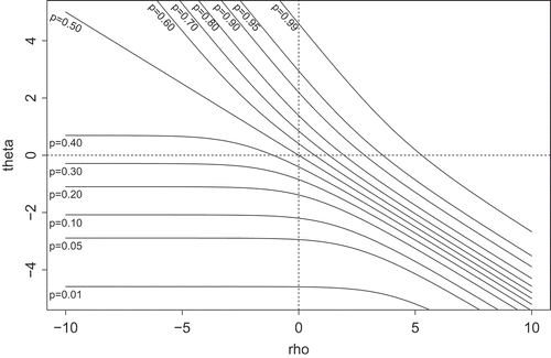
As Figure 1 illustrates, in the model the parameters and have differently shaped negative relations for different values of the probability of a tie . Both and are also related to since for larger values of both increase. When , equals the log odds of . For values , is larger than the log odds of while the opposite holds for .

2.2 The model

The new model applies probabilities to the different dyadic outcomes through the density parameter and a parameter which is indirectly used to model the reciprocity:

(5)

with

The density parameter models the log odds of a single tie, which can be seen by solving Equation (5) for ,

(6)

The reciprocity parameter in the model, , is similar to the expression for in the model (Equation (4)),

(7)

The values for in Equation (5) and thus the probabilities for the dyadic outcomes can be determined after solving for as

In the model, only depends on and consequently is independent of . Any differences in as a result of differences in are subsequently also independent of . In summary, the model has a density parameter for the log odds of and an independent reciprocity parameter for the log odds ratio (Equation (7)).

2.3 The model

The model (Van Duijn 1995; Van Duijn et al., 2004) took a major step forward by extending the model (Holland and Leinhart, 1981) to allow predictor variables for the sender and receiver effects and for density and reciprocity. This was achieved by introducing random sender and receiver effects, freeing up parameter space for the coefficients of the predictors. The model extends on the model analogously to the extension of the model on the model.

The density parameter is substituted by random sender and receiver effects and and an overall parameter for the log odds of . The random effects are assumed to have a bivariate normal distribution with variances , and covariance . The density parameter is further substituted by the regression parameters , , and for sender, receiver, and density predictors , , and , respectively,

The sender and receiver predictors are variables at the actor level and the density predictors are variables at the dyad level.

The parameter for reciprocity (Equation (7)) is substituted by an overall estimate of reciprocity and regression coefficients for symmetric dyadic predictors, ,

3. Estimation and prior distributions for the model

In logistic regression, estimates can become highly unstable due to a phenomenon called separation (Albert and Anderson 1984). This stems from sparse data being (nearly) identified for one of the outcomes. This is also observed in the and models, in particular with the extended specification of the reciprocity parameters and in the model. Since these are independent of the probability of a tie , they are relatively unstable. One way to deal with this problem is to apply an appropriate prior distribution in Bayesian simulation methods. For this reason the model is estimated with an Markov chain Monte Carlo (MCMC) algorithm (see e.g. Gelman et al. 2014), subsequently sampling the random effects , their covariance matrix , and the regression parameters . The prior distribution applied to is an inverse Wishart distribution. 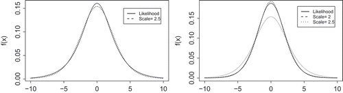Since the model closely resembles logistic regression for the parameters , , , and in , their prior distribution is based on assuming half an observation for each outcome in logistic regression, as suggested by Gelman et al. (2008). This results in the likelihood

closely resembling a -distribution with 7 degrees of freedom and scale 2.5 (see Figure 2), which was taken as the actual prior distribution. In a similar manner, a prior distribution for the parameters and in was derived. However, the prior based on assuming half an observation for all dyads still resulted in unstable estimates. Therefore, the prior distribution was based on the likelihood assuming one observation for each dyad (and ),

This distribution is close to a -distribution with 7 degrees of freedom with scale 2 (see Figure 2), which was applied as prior distribution.

Figure 2. Likelihoods serving as reference for the prior distributions for m, γ₁, γ₂ and γ₃ (left) and r and γ₄ (right) and approximating t-distributions with df = 7.

For the regression parameters , , , and , the above priors were further adjusted to the variation in the predictors through dividing the scale of the -distributions by the observed standard deviation of , , , and . Following Raftery (1996) and Gelman (2008), the predictors were centered to an average of zero to assure the center of the prior distributions can be set at zero as well.

4. Simulations

To verify the effectiveness of the prior distributions against separation, simulations were run. Data were simulated according to model 3 from Zijlstra et al. (2009), containing predictors at the actor level (for receiving) as well as at the dyad level (for density and reciprocity). The variance of the random sender effects () was taken twice as large as the variance of the random receiver effects () with a negative covariance (). The density and reciprocity were and , corresponding to . A receiver effect with coefficient was added for a predictor drawn from a binary (0,1) distribution with equal probabilities. There are two density predictors; is the coefficient for a predictor drawn from a multinomial distribution with five outcomes (1, 2, 3, 4, 5) with equal probability and is the coefficient for a random digraph with . Finally, the coefficient for the predictor for reciprocity, , represents the effect of the absolute differences of the multinomial outcomes used as a predictor for the density. Different values for were applied. A very small value of was based on Zijlstra et al. (2009). To have a more complete test for separation, a substantial value of , implying a predicted range of 4 for the log of Equation (4), and a large value , implying a predicted range of 8 for the log of Equation (4), were used as well. All models were simulated 1,000 times for relatively small networks of 20 actors and medium-sized networks of 40 actors. The -distribution with was used as prior, with scales as described in Section 3. Results are presented in Table 1. Here, only is reported for the models with simulated values and because results for the other parameters were highly similar to those in the model with .

Table 1. Mean parameter estimates, posterior standard deviations,and coverage rates of the 95% and 99% coverage intervals over 1,000 replicated networks.

		20 actors				40 actors
Effect	Simulated value	Mean	SD	95	99	Mean	SD	95	99
Receiver		–0.087	0.490	0.938	0.987	–0.102	0.287	0.930	0.982
Density		–1.453	0.184	0.947	0.995	–1.433	0.091	0.945	0.984
		0.203	0.154	0.927	0.987	0.199	0.074	0.931	0.989
		0.509	0.337	0.972	0.988	0.492	0.160	0.971	0.994
Reciprocity		1.892	0.716	0.957	0.992	1.990	0.322	0.945	0.991
		0.127	0.672	0.961	0.993	0.092	0.296	0.948	0.988
		0.962	0.755	0.963	0.995	1.028	0.365	0.953	0.993
		1.658	0.866	0.945	0.986	1.938	0.480	0.962	0.992
Random effects
Sender variance		1.629	0.761	0.938	0.993	1.535	0.433	0.949	0.991
Receiver variance		0.941	0.459	0.970	0.997	0.822	0.242	0.953	0.989
Sender–receiver covariance		–0.477	0.404	0.937	0.986	–0.507	0.232	0.944	0.990

For the regression parameters, all coverage rates in Table 1 are relatively close to the nominal values of 95 and 99. This indicates that even for small networks of 20 actors the prior distributions for the regression parameters yield acceptable intervals for inference, avoiding separation. However, for the small networks the average point estimates for and are relatively far from their simulated values. This appears to be mainly due to the large standard deviations for these parameters. For the medium-sized networks of 40 actors, the standard deviations are smaller and the point estimates are relatively close to their simulated values.

5. Application: reported emotional support between Dutch high school pupils

To further illustrate the model, it was applied to a network from the Dutch Social Behavior Study (Baerveldt and Snijders 1994; Baerveldt et al. 2004). The network was measured on a year group of 62 high school students with 37 boys and 27 girls of ages between 16 and 18 years old. Each student was asked from whom they had received emotional support when they were depressed, for instance, after the end of a relationship or in a conflict with someone else. Two models were estimated. In model 1, a sender and receiver effect for being a boy is included as well as a density effect for (dyads of) different gender. In model 2, a reciprocity effect for different gender is added.

Results are presented in Table 2. For the model, a negative receiver effect is found for being a boy. This indicates that the probability of reporting having received emotional support from boys is smaller compared to girls. There is an additional negative density effect for “different gender,” indicating a smaller probability of receiving emotional support in dyads with different gender. Thus, given the receiver effect of “boy,” receiving emotional support from someone of similar gender is more likely. In model 2, no further effect of different gender on the reciprocity is found.

Table 2. Estimates with posterior standard deviations for reported emotional support for and models.

		Model 1		Model 2		Model 1		Model 2
Effect	Predictor	Est.	SD	Est.	SD	Est.	SD	Est.	SD
Sender	Boy ()	–0.22	0.36	–0.24	0.35	0.00	0.45	–0.17	0.37
Receiver	Boy ()	–1.01	0.33	–1.02	0.32	–1.05	0.38	–0.95	0.31
Density ()		–4.60	0.21	–4.59	0.22	–5.32	0.26	–5.15	0.25
	Different gender ()	–1.17	0.33	–1.15	0.32	–0.80	0.25	0.05	0.11
Reciprocity ()		5.07	0.67	5.18	0.61	4.84	0.51	4.35	0.61
	Different gender ()			0.82	1.79			–1.52	0.68
Random effects
Sender variance ()	0.73	0.27	0.70	0.30	0.92	0.34	0.75	0.34
Receiver variance ()	0.43	0.19	0.45	0.21	0.36	0.20	0.35	0.15
Sender–receiver covariance ()	0.26	0.19	0.30	0.22	–0.17	0.19	0.11	0.19

For , estimates for analogue models are presented in Table 2 as well. A similar receiver effect of “boy” and density effect of “different gender” was found on the odds of an asymmetric versus a null dyad. However, in model 2, the density effect of different gender is no longer significant, while there is now a significant negative reciprocity effect (assuming a significance level of 0.05). This is unexpected since the observed log odds ratio for different gender (Equation (2)) is actually higher (6.14 compared to 5.03 for same gender). In the model, such effects are possible since the sender, receiver, density, and reciprocity effects are all dependent on each other and jointly model the observed data (see also Figure 1).

Comparing between models, the standard deviation for the coefficient of the predictor for reciprocity, , is particularly large in the model. This originates from the reciprocity parameters and γ₄ in partly modeling the probability . In contrast, in the reciprocity parameters are independent of , resulting in less stable estimates.

6. Concluding remarks

With , a new model for regression of predictors on dichotomous dyadic network data was introduced. This was compared to the most similar model, the model. Both can be preferred in different situations. An advantage of is that the density and reciprocity parameters are independent, avoiding ambiguous estimates as seen for the model in the application in Section 5. Besides, the parameter for density in the model has a familiar interpretation as the log odds of a tie, comparable to logistic regression. On the other hand, when there is theoretical interest in non-reciprocated ties, the model seems to be most appropriate because the density parameter in estimates the odds of asymmetric dyads.

A property of the model that requires further investigation is that the estimation of the reciprocity parameter is unstable because of the independence from the density parameter. With the introduction of specific prior distributions, a practical solution to this problem was presented. However, an analytical solution may further improve the estimates.

For the and model, the dependence between the density and reciprocity also requires further investigation. Even though it applies the same expression for reciprocity (Equation (4)) as the and model (Equation (7)), it is not yet clear how specifically the interpretation is affected by its dependence on density. Because the reciprocity parameter in the and model is related to the probability of a single tie, the frequency of symmetric dyads, that is, (1,1), is modeled to a greater extent by the reciprocity parameter than the frequency of null dyads, that is, (0,0). On the contrary, given the probability of a single tie, the and model assign equal weight to both null and symmetric dyads. These models may therefore be of particular value in cases where there is substantial theoretical interest in the extent to which both null and symmetric dyads are observed beyond chance.

Software for estimating models is freely available from the corresponding author. The R-package (R Core Team 2014) dyads is expected to become available in the near future.

References

- Albert, A., and J. A. Anderson. (1984). On the existence of maximum likelihood estimates in logistic regression models. Biometrika, 71(1), 1–10.
- Baerveldt, C., and T. A. B. Snijders. (1994). Influences on and from the segmentation of networks: Hypotheses and tests. Social Networks, 16, 213–232.
- Baerveldt, C., M. A. J. Van Duijn, L. Vermeij, and D. A. Van Hemert. (2004). Ethnic boundaries and personal choice. Assessing the influence of individual inclinations to choose intra-ethnic relationships on pupils networks. Social Networks, 26, 55–74.
- Gelman, A. (2008). Scaling regression inputs by dividing by two standard deviations. Statistics in Medicine, 27(15), 2865–2873.
- Gelman, A., J. B. Carlin, H. S. Stern, and D. B. Rubin. (2014). Bayesian data analysis (Vol. 2). Boca Raton, Florida, USA: Chapman & Hall/CRC.
- Gelman, A., A. Jakulin, M. G. Pittau, and Y. S. Su. (2008). A weakly informative default prior distribution for logistic and other regression models. The Annals of Applied Statistics, 2(4), 1360–1383.
- Holland, P. W., and S. Leinhardt. (1981). An exponential family of probability distributions for directed graphs. Journal of the American Statistical Association, 76, 33–50.
- R Core Team. (2014). R: A language and environment for statistical computing. R Foundation for Statistical Computing: Vienna, Austria. http://www.R-project.org/
- Raftery, A. E. (1996). Approximate Bayes factors and accounting for model uncertainty in generalised linear models. Biometrika, 83(2), 251–266.
- Robins, G., P. Pattison, Y. Kalish, and D. Lusher. (2007). An introduction to exponential random graph (p*) models for social networks. Social Networks, 29(2), 173–191.
- Van Duijn, M. A. J. (1995). Estimation of a random effects model for directed graphs. In: SSS95. Symposium Statistische Software, 7, 113–131.
- Van Duijn, M. A. J., T. A. B. Snijders, and B. J. H. Zijlstra. (2004). P2: A random effects model with covariates for directed graphs. Statistica Neerlandica, 58, 234–254.
- Zijlstra, B. J. H., M. A. J. Van Duijn, and T. A. B. Snijders. (2009). MCMC estimation for the P2 network regression model with crossed random effects. British Journal of Mathematical and Statistical Psychology, 62, 143–166.