Sensitivity analysis of a passive decay heat removal system under a post-loss of coolant accident condition

Abstract

Passive safety features are now of interest to the design of future generation reactors because of their peculiar characteristics of simplicity, reduction of human interaction, and avoidance of failures of active components. However, the large uncertainty associated with the responses of passive systems might not be ignored. Therefore, it is necessary to identify the uncertain inputs that have the important impact on the uncertainty of the system performance. In this study, two global sensitivity measures, the first-order sensitivity index and the total-order sensitivity index, are applied to a natural circulation decay heat removal system of a gas-cooled fast reactor for identifying the important system inputs. It is found that the uncertainty in the system pressure contributes the most to the uncertainty in the system outputs. In addition, the cooler (the heat exchanger of the emergency cooling system) wall temperature, the Nusselt number in the mixed convection regime, and the friction factor in the mixed convection flow regime also have small impact on the uncertainty of the system outputs.

Keywords:

• sensitivity
• uncertainty
• nuclear power generation safety
• passive safety systems
• sensitivity analysis

1. Introduction

Passive safety features are now of interest to the design of future generation reactors. They are characterized by their full reliance upon natural laws (e.g., gravity, natural circulation, heat conduction, and stored energy) to accomplish their designated safety functions. However, the large uncertainties associated with passive systems are acknowledged [1 –6]. These uncertainties are due to the lack of understanding of the underlying phenomena of these systems as well as the lack of operating experience of these systems. Up till now, some efforts have been done for quantifying the uncertainty of the performance of passive safety systems and for estimating their failure probabilities [1 –6]. If the uncertainty of the system performance is large, it is necessary to know where further efforts should be focused so that this output uncertainty can be reduced. Sensitivity analysis plays an important role for identifying the important inputs that have the important impact on the uncertainty of the system performance.

The design of a 600 MW gas-cooled fast reactor (GFR) has been the subject of study at the Massachusetts Institute of Technology (MIT) in the past several years [7 –11]. A natural convection cooling system has been designed for decay heat removal and a steady-state model of this system has been developed. The input parameters of this model include the reactor power level, the system pressure, the cooler (the heat exchanger (HX) of the emergency cooling system (ECS)) wall temperature, and the correlations for describing the thermal-hydraulic phenomena. Two outputs of the system are the helium gas coolant temperatures at the outlet of the hot channel and the average channel, respectively. In this work, by evaluating the contribution of each uncertain input to the uncertainty in the outputs, we aim to identify the key inputs affecting the output uncertainties for further improving the model and the design of this reactor.

This paper is organized as follows. In Section 2, with the comparison of several sensitivity analysis methods, two global sensitivity measures are adopted for sensitivity analysis of this decay heat removal system. Then, the extended Fourier amplitude sensitivity test (FAST) method for calculating these two measures is introduced in Section 3. In Section 4, the model of this natural convection system is described in detail. The sensitivity analysis results and discussions are presented in Section 5. Finally, conclusions are given in Section 6.

2. Sensitivity analysis methods

2.1. Local sensitivity analysis methods

A local sensitivity analysis method is conceived and often defined as a local measure of the effect of a given input on a given output. Given a model Y = g(X), where Y is the model output of interest, and X = {X ₁, X ₂, … , X_m } (m is the number of input parameters) is the set of uncertain input parameters, a Taylor series approximation to Y can be developed. If we restrict this series to first-order terms, we have the approximation:

where X₀  = [x ₁₀, x ₂₀, … x_{m 0}] is the set of nominal values of input parameters.

The common way to describe a local sensitivity coefficient is that it is the first-order partial derivative of the model output with respect to the model input, which is expressed as

in Equation (2) is calculated by varying the input parameter X_i , while fixing all other inputs at their nominal values. Since depends on the units used for the input parameters, its unit will change when the units of input parameters change. Therefore, should be normalized in order to remove the effect of the units. The approximation in Equation (2) can be rewritten in the two following forms:

Two normalized expressions of are then defined as

and

where y ₀ = g(X₀) and and σ _y are the standard deviations of the input parameter X_i and the model output Y, respectively.

measures the effect on Y that results from perturbing X_i by a fixed fraction of its nominal value . measures the effect on Y which results from perturbing X_i by a fixed fraction of its standard deviation. From the definition of , , and , it is known that only a small perturbation of X_i in the neighborhood of its nominal value is permitted for calculating the partial derivative. Because the value of an input parameter could be any value in its distribution range, it is necessary to take the entire distribution of this parameter into consideration. This is done through global sensitivity analysis, which looks at the output uncertainty over the entire distributions of the input parameters.

2.2. Global sensitivity analysis methods

A global sensitivity analysis method evaluates the effect of an input parameter on the uncertainty of the model output by looking at the entire distribution of this input. Several global sensitivity measures have been proposed [12 –17]. Among them, the first-order sensitivity index [14] and the total-order sensitivity index [15] are popularly used.

In statistics, variance (as well as standard deviation) has been a universal term to represent data variation. With the implicit assumption that the uncertainty of a model output could be represented by its variance, Hora and Iman proposed a global uncertainty importance measure [12]. It is given as

where V(Y) is the variance of the model output Y when all input parameters are sampled from their probability distributions, and is the expected variance of Y that remains if the input parameter of interest X_j was known. Here, X _−j means all input parameters except X_j are included.

The expected percentage reduction of the variance of Y is obtained as follows [13]:

where represents the variance that is expected to be reduced when the value of X_i was known. Here, X _−i means all input parameters except X_i are included.

From statistical science, we know that the relationship holds. Equation (8) is in fact the definition of the first-order sensitivity index S_i proposed by Sobol [14]. When the input parameters are independent, based on Sobol's variance decomposition procedure [14], V(Y) is decomposed as follows:

where , , and so on.

The Sobol's sensitivity indices are defined as

According to Equation (9), satisfy

Each index is a sensitivity measure describing the percentage of the total variance contributing to the uncertainties in the set of input parameters . S_i is named as the first-order index, S_ij is named as the second-order index, and so on. S_i describes the effect of parameter i on the variance of Y when it is taken alone. The higher-order indices account for interaction effect of various parameters on the variance of Y.

When there are no interactions among input parameters, it is known from Equation (11) that

In this case, S_i is enough to identify the input that contributes the most to the variance of the model output. However, it is a fact known to both modelers and experimentalists that the number and importance of the interaction terms between input parameters usually grow with the number of input parameters [18]. Therefore, it is also necessary to describe the contribution of these interaction terms to the variance of the model output. If a model has m input parameters, it is known from Equation (11) that the total number of sensitivity indices to be calculated is as high as 2 ^m  − 1, which increases exponentially with the number of input parameters. This brings about the computational problem referred to as the curse of dimensionality [19]. To cope with this dimensionality problem, the total effect sensitivity index S_Ti has been proposed [15]. It is defined as the sum of all partial sensitivity indices involving parameter X_i . For example, in a model with four input parameter Y = g(X ₁, X ₂, X ₃, X ₄), the total effect index involving parameter X ₁ is

It can be proved that

where X _−i means all input parameters except X_i are included.

S_Ti measures the total effect of an input parameter. It represents the expected percentage of the variance of the model output that remains if all input parameters except X_i were known. For a given input parameter X_i , the difference between S_i and S_Ti shows the effect of the interaction terms involving X_i on Y. If S_i is high, we know that X_i has an important effect on the variance of Y. If S_i is small and S_Ti is high, we know that the effect of X_i on the variance of Y is mainly through the interaction terms involving X_i . If both S_i and S_Ti are small, we know that X_i has a negligible effect on the uncertainty of Y.

S_i and S_Ti are the most popularly used global sensitivity measures and have been applied to many different models [20]. Both measures are used in this study for identifying the important model inputs of a thermal-hydraulic model. In the next section, the method for computing S_i and S_Ti will be introduced.

3. The extended FAST method

The FAST method was introduced in 1970s for computing S_i [21 –24]. It was extended by Saltelli et al. for computing both S_i and S_Ti [25]. The core idea of FAST is to assign each input parameter X_i an integer frequency ω _i through a search curve G_i (sin(ω _is)), which is used to explore the multidimensional space of the model inputs:

where s is a scalar variable varying over the range −π < s < π, and G_i (sin(ω _is)) satisfies

where u = sin(ω _is) and P_i (G_i (u)) is the probability density distribution (PDF) of G_i (u).

Equation (16) can be transformed to the following equation:

Integrating both sides of Equation (17), we have

where Γ _i is the cumulative distribution function of G_i (u) and C is a constant.

G_i (u) can then be obtained as follows:

where is the inverse function of Γ _i .

When the input parameter X_i is uniformly distributed, based on Equations (15) and (19), we have

If X_i is uniformly distributed in [0, 1], C will be 0.5.

The model output Y can be expanded by using a Fourier series:

where

Here, T is the period of Y, and i ∈ {−∞,…, − 1,0,1, … , + ∞}.

If ω _i s are positive integers, the period T will be 2π. Equations (22) and (23) then become

For practical problems, A_i and B_i can be computed by using discrete sampling techniques. Suppose we sample s from the range (−π, π), we have

where

Based on Equation (15), we can obtain a set of input parameters for each s_i ,

and calculate the model output.

Equations (28) and (29) are repeated n times; finally, we can obtain the Fourier coefficients:

A_i and B_i have the following properties:

Especially, when i = 0, we know

The spectrum of the Fourier series expansion is defined as

where i ∈ {−∞,…, − 1,0,1, … , + ∞}.

We have

The variance of Y is

By evaluating the spectrum for the frequency ω _i and its higher-order harmonics pω _i (p ∈ { − M,…, −1,0,1,…, M}, M is the number of harmonics considered in the analysis, which is usually set to 4), the partial variance of Y arising from the uncertainty of the input parameter X_i can be estimated by

The first-order sensitivity index S_i can then be obtained by calculating V_i /V(Y).

To calculate the total-order sensitivity index S_Ti , the input parameter X_i needs to be assigned a high integer frequency ω _i , while the other input parameters except X_i are assigned low frequencies in the range (1, ω _i /2) [25]. A Fourier analysis allows the sum of all the terms that do not include the parameter X_i (let us indicate it as V _−i ) to be recovered at the low end of the spectrum:

The quantity V(Y) − V _−i is the sum of all effects involving X_i , i.e., the effects needed for computing S_Ti . S_Ti can then be obtained by calculating 1 − V _−i /V(Y).

4. The case study

4.1. System descriptions and operating conditions

The case in this study is a three-loop natural convection cooling system of a conceptual GFR under a post-LOCA condition [4]. The reactor is a 600 MWth GFR cooled by helium flowing through separate channels in a silicon carbide matrix core. This design has been the subject of study in the past several years at MIT within the framework of the I-NERI project Development of GEN IV Advanced Gas-Cooled Reactors with Hardened/Fast Neutron Spectrum [7 –11].

One loop of a GFR decay heat removal configuration is shown schematically in Figure 1. The flow path of the cooling helium gas is shown by the black arrows. The hot helium gas from the reactor core proceeds through a top reflector and chimney to the inner coaxial duct and then upward to the hot plenum of the ECS HX, where it transfers heat to naturally circulating water on the secondary side. The cold helium gas from the HX flows down through a check valve to the outer coaxial duct, which brings it back to the reactor vessel, where it proceeds through the downcomer back to the reactor core. A check valve (item 15 in Figure 1) is installed to prevent backflow through the HX during normal operation. A blower is mounted in the downcomer below the HX to provide cooling during shutdown, since the safety grade ECS HX is used for shutdown cooling and post-LOCA heat removal. In order to achieve a sufficient decay heat removal rate by natural circulation, it is necessary to maintain an elevated pressure even after the LOCA. This is accomplished by a guard containment, which surrounds the reactor vessel and power conversion unit and holds the pressure at a level that is reached after the depressurization of the system.

Figure 1. Schematic representation of one loop of the GFR passive decay heat removal system [4].

The three heat removal loops are identical in geometry and characteristics. The loop dimensions are summarized in Table 1, where the section number in the first column corresponds to the flow path number in Figure 1.

Table 1. Geometric parameter of the system [4].

Section	Hydraulic diameter (m)	Flow area (m^2)	Length (m)	ΔZ* (m)	K loss coefficient	Roughness (m)
1	0.6	7.2571	7.7	−5.3	1	4.5 × 10^−5
2	7.4	43.008	1	0.5	0	4.5 × 10^−5
3	0.0145	1.65 × 10^−4	1	1	0.5	1.0 × 10^−5
4	0.0145	1.65 × 10^−4	1.7	1.7	0.25	1.0 × 10^−5
5	0.0145	1.65 × 10^−4	1	1	1	1.0 × 10^−5
6	7.4	43.0	3	3	0	4.5 × 10^−5
7	5.4	22.9	6	6	0.1	4.5 × 10^−5
8	0.8	50.3	4	0	1.23	4.5 × 10^−5
9	1	2.24	2	2	0	4.5 × 10^−5
10	1.6364	5.4	1.5	1.5	0.1	4.5 × 10^−5
11	0.15	1.35	1.25	−0.5	0.23	4.5 × 10^−5
12	0.003055	9.81	0.3	−0.3	1.23	1.0 × 10^−5
13	0.15	1.35	1.25	−0.2	1	4.5 × 10^−5
14	1.526	8.2	1	−1	0	4.5 × 10^−5
15	1	3.76	3	−3	13.23	4.5 × 10^−5
16	1.526	8.20	1	−1	0	4.5 × 10^−5
17	0.25	0.363	3	0	1	4.5 × 10^−5
18	2.0253	2.29	5.4	−5.4	0.5	4.5 × 10^−5
Notes: *It refers to the change in height from the beginning to the end of the section in question. “−” signal represents that the height of the end of a section is lower than the height of the beginning of this section.

The average core power to be removed is assumed to be 12 MWth, which is equivalent to 2% of the full reactor power. The work by Hejzlar [7] and Okano et al. [8] has shown that this percent is a reasonable approximation. To guarantee natural circulation cooling at this power level, a pressure of 1650 kPa is required [4]. In addition, the secondary side of the HX is assumed to have a nominal wall temperature of 90°C.

It is important to note that the subject of the present analysis is the steady-state natural circulation cooling that takes place after the LOCA transient has occurred. Our purpose is to identifying the important variables that affect the stability of the functionality of a long-term decay heat removal. Therefore, the analysis hereafter refers to this steady-state period.

4.2. The thermal-hydraulic model

To simulate the steady-state behavior of this decay heat removal system, a thermal-hydraulic code developed at MIT has been used [7]. This code treats all multiple loops as identical, and each loop is divided into 18 sections that are defined by their length, hydraulic diameter, surface area, height, form loss coefficient and roughness. The heater (i.e., the reactor core, item 4 in Figure 1) and the cooler (i.e., the HX, item 12 in Figure 1) have been further subdivided into 40 separate nodes to calculate the temperature and flow gradient in detail. Both the average and the hot channels are modeled in the core so that an increase in temperature in the hot channel due to the radial peaking factor can be calculated.

To obtain a steady-state solution, the code balances the pressure losses around the loop so that friction and form losses are compensated by the buoyancy term, while at the same time maintains the heat balance in the heater and the cooler. The heat balance between the inlet and outlet of each node in the heater and the cooler is calculated through Equation (41):

where [Qdot] _i is the heat rate in the ith node (kW), [mdot] _i is the mass flow rate in the ith node (kg/s), c_{p ,i} is the specific heat at constant pressure in the ith node (kJ/(kg K)), T_i is the temperature measured at the outlet of the ith node, the inlet, the wall channel, and the coolant bulk (K), S_i is the heat-exchanging surface in the ith node (m²), and h_i is the heat transfer coefficient (kW/(m² K)) in the ith node.

Equation (41) describes the equality between the enthalpy increase of the flow from the inlet to the outlet in a node and the heat exchange from the channel wall to the bulk of the coolant. The heat transfer coefficient h_i is determined by Nusselt number, which is a function of fluid characteristics and geometry, and is calculated through appropriate correlations covering forced, mixed, and free convection regimes in both turbulent and laminar flow, as reported in Williams et al. [10,11].

The mass flow rate is determined by a balance between the buoyancy and pressure loss along the closed loop:

where ρ _i is the coolant density in the ith section (kg/m³), H is the height of the ith section, f_i is the friction factor in the ith section, L_i is the length of the ith section, D is the hydraulic diameter of the ith section (m), [mdot] is the mass flow rate in the ith section, A_i is the flow area of the ith section (m²), and K is the form loss coefficient.

Equation (42) states that the sum of buoyancy (first term), friction losses (second term), and form losses (third term) is equal to zero along the closed loop in the steady state. The friction factor f_i is a function of the fluid characteristics and geometry and is calculated using appropriate correlations, as reported in Williams et al. [10].

The assumptions employed in the model are summarized as follows:

•	Steady-state natural flow;
•	The helium gas flow is one dimensional, fully developed;
•	Temperature on the walls of the HX and the reactor core is considered uniform along both axial (within the node) and azimuthal coordinates;
•	The contribution of radiation is neglected;
•	The duct walls are perfectly insulated on the outside; and
•	Gas properties are temperature dependent and are evaluated at operating pressure (local pressure variation due to pressure losses is not accounted for in property equations);

An iterative algorithm was used to find a solution that satisfies simultaneously the heat balance and pressure losses equations. The calculations begin with a guess of temperature distribution along the loop and the estimate of the mass flow rate for the calculation of gas properties. Then, the mass flow rate is iteratively solved to satisfy continuity in the closed loop. Next, the reactor core section is solved using the heat transfer coefficient from the updated mass flow rate. Since the heat transfer coefficients also depend on gas temperatures, iteration loops on the reactor core heat balance are necessary. Once the core outlet temperature is determined, it is used as the inlet temperature to the HX to solve iteratively for HX outlet temperature and to satisfy the heat balance in the HX. Finally, the HX outlet temperature is compared to the reactor core inlet temperature. If they do not agree, an adjustment to the reactor core inlet temperature will be made and the whole process will be repeated starting with new mass flow rate evaluation. Iterations proceed until the difference between the HX outlet and the reactor core inlet temperatures is smaller than a user-prescribed tolerance (typically 0.01°C).

4.3. Uncertainties in the thermal-hydraulic model

The thermal-hydraulic model introduced in the previous section is a simplified mathematical representation of the steady-state behavior of the natural decay heat removal system. To what extent the model result predicts the reality depends on the accuracy of the phenomena described in the model and on the accuracy of the values of parameters being used. The uncertainty associated with the model is call model uncertainty, and the uncertainty associated with the parameters is known as parameter uncertainty. Both types of uncertainty are due to the lack of knowledge of the phenomena being modeled and the parameters adopted. Hence, they are referred to as epistemic uncertainty.

In this thermal-hydraulic model, model uncertainty is related to the correlations adopted to describe the thermal-hydraulic phenomenon (e.g., friction factor and Nusselt number). Since the models used for calculating the correlations are just simplified representation of the real phenomenon, the uncertainty of the model can be described by a multiplicative model [26]:

where y is the real value of the quantity to be predicted, f(x) is the result of the correlation, and ε is the error factor.

Based on Equation (43), the uncertainty in the quantity y is then translated into the uncertainty in the error factor ε . In the preceding work by Pagani et al. [4], two parameters that have to be calculated from existing correlations; that is, Nusselt number and friction factor were selected to represent the uncertainties with this thermal-hydraulic model. Nusselt number is directly related to heat transfer coefficient, which affects the helium gas temperatures in the reactor core and the HX, as shown in Equation (41). Friction factor is directly related to the pressure loss, which affect the mass flow rate of helium in the system, as shown in Equation (42). Because the helium gas works in different flow regimes, as reported by William et al. [10,11], the parameters Nusselt number and friction factor are further divided based on the characteristics of the flow regimes, i.e., the forced convection regime, the mixed convection regime, and the free convection regime.

In addition, the reactor core power level, the system pressure, and the cooler wall temperature were identified as the three parameters that are associated with parameter uncertainty, as reported by Pagani et al. [4].

The consideration of these uncertainties leads to a definition of nine uncertain input parameters for this model. As shown in Table 2, the uncertainties of these parameters have been represented by normal distributions. Their mean value and the standard deviations were also given [4]. The uncertainty distributions used represent the current state of knowledge of the uncertainties of these parameters by its research group. It is conceivable that they might change in the future as more experimental data are obtained and more knowledge is accumulated. The choices of these parameters and their distributions are elaborated below.

Table 2. Uncertain parameters in the GFR passive decay heat removal system.

	Parameter	Mean value	Standard deviation (% of the mean value)
Parameter uncertainty	X 1 (power level (MW))	12.0	1
	X 2 (system pressure (kPa))	1650	7.5
	X 3 (cooler wall temperature (°C))	90	5
Model uncertainty (ε)	X 4 (Nusselt number in the forced convection regime)	1	5
	X 5 (Nusselt number in the mixed convection regime)	1	15
	X 6 (Nusselt number in the free convection regime)	1	7.5
	X 7 (friction factor in the forced convection regime)	1	1
	X 8 (friction factor in the mixed convection regime)	1	10
	X 9 (friction factor in the free convection regime)	1	1.5

4.3.1. Power

According to industry practice and experience, an error of 2% is usually considered in the determination of the power level, due to uncertainty in the measurement. Assuming that this error defines the 95% confidence interval, the standard deviation equal was set to 1% [4].

4.3.2. Pressure

The system pressure before the accident is kept by the control system within a small percentage of the nominal value. However, the post-LOCA conditions are determined not only by the pressure level in the primary system and guard containment before the accident but also by the energy stored before the accident, the energy absorbed by surrounding materials, the dynamics of the accident, and by the leakage rate of the gas from the guard containment. All these uncertainties accumulate in the final pressure value in the guard containment. Therefore, its uncertainty in post-LOCA conditions should be relatively large and the 95% confidence interval was set to ±15% [4].

4.3.3. Cooler wall temperature

In this thermal-hydraulic model, the inner wall (the wall in contact with the helium gas) temperature in the HX was used as a boundary. Water with inlet and outlet temperature of 25°C and 85°C, respectively, was proposed as the secondary cooling medium. The design of secondary cooling system has not been finalized; hence, a uniform inner wall temperature of 90°C was used in the model as an approximation. This wall temperature will be affected by the variation in inlet water temperature of the second side of the HX, which arrives from the storage tank outside the guard containment and is affected by ambient conditions in the reactor building. Considering the uncertainties of the second side of the heat exchange, a 95% confidence interval of ±10% on this vale was considered [4].

4.3.4. Nusselt number and friction factor

Correlations used to calculate the Nusselt numbers and friction factors are obtained from experimental databases. They have different functional forms depending on the geometry, fluid characteristics, boundary conditions (uniform heat or uniform temperature), and fluid regimes (forced, natural, or mixed convection). Heating in vertical piping and the forced flow regime has been extensively studied because of its practical importance in power production, and the correlations involved are quite precise. On the other hand, natural and especially mixed convection correlations are not supported by extensive experimental results, and the resulting correlations suffer from larger uncertainty. Starting from correlation errors available in the literature [27,28], and depending on the applicability of the correlation used, the error on the Nusselt number was estimated to range from a minimum of 10% (forced convection) to a maximum of 30% (mixed convection) [4]. Similarly, the error on the friction factor ranges from a minimum of 2% (forced convection) to a maximum of 20% (mixed convection).

5. Results and discussions

For the GFR passive decay heat removal system, a configuration of three loops was considered in the analysis. Two model outputs were taken into consideration. One is the helium gas temperature at the outlet of the hot channel in the reactor core (denoted as Y ₁ herein). The other is the helium gas temperature at the outlet of the average channel in the reactor core (denoted as Y ₂ herein). The difference between the average channel and the hot channel is that the radial peaking factor is considered in the latter.

5.1. Uncertainty analysis of the model outputs

As introduced in Section 2.2, the first-order sensitivity index S_i and the total-order sensitivity index S_Ti are established with the assumption that variance is enough to represent uncertainty. If the distributions of the model outputs are normal (or nearly normal), S_i and S_Ti are applicable to them. If the distributions of the model outputs are highly skewed, variance will not be suitable to represent uncertainty. In this case, other sensitivity indices, such as the indicator proposed by Liu and Homma [17], might be suitable.

To check the shapes of the distributions of the model outputs, uncertainty analysis was firstly performed. We randomly sampled 100,000 sets of the input parameters and propagated them through this thermal-hydraulic model. The obtained distributions of Y ₁ and Y ₂ are shown in Figures 2 and 3, respectively. It is known from both figures that the distributions of Y ₁ and Y ₂ are almost symmetric about the means. The mean of Y ₁ and Y ₂ are about 638°C and 497°C, respectively. Therefore, S_i and S_Ti are applicable to this model.

Figure 2. The PDF of the helium gas temperature at the outlet of the hot channel.

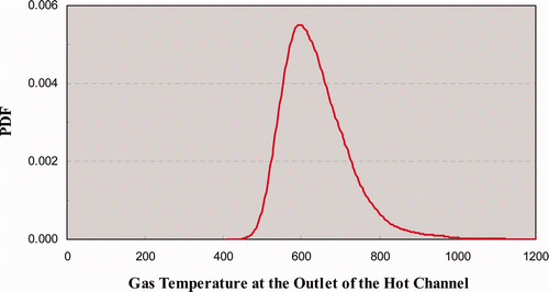
Figure 3. The PDF of the helium gas temperature at the outlet of the average channel.

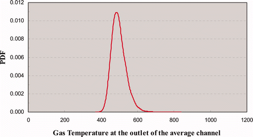
In addition, it is obvious that the distribution of Y ₁ is wider than that of Y ₂. The standard deviation of Y ₁ is 84.6°C. It is about 2.2 times larger than that of Y ₂, which is 39.2°C. This means that the variations of system pressure, Nusselt numbers, and friction factors have more impact on the helium gas temperature in the hot channel than that in the average channel. Because of the effect of radial peaking in the hot channel, the gas temperature in the hot channel is higher than that in the average channel. Therefore, the kinematic viscosity in the hot channel is higher. The study by Williams et al. [11] has shown that the helium gas flow in the core works in the laminar regime, where the friction factor is inversely proportional to the Reynolds number:

where u_f is the velocity of helium gas (m/s), d is the hydraulic diameter of the channel (m), and ν is the kinematic viscosity (m²/s). Therefore, the friction factor in the hot channel is larger than that in the average channel. In addition, the density of helium gas in the hot channel is smaller than that in the average channel. Based on Equation (42), we know that it is more difficult to maintain the balance between the buoyancy and pressure loss in the hot channel than in the average channel. Hence, it is easier to lead to the change of the helium gas flow rate and temperature in the hot channel than in the average channel if there are variations of system pressure, Nusselt numbers, and friction factors.

5.2. Ranking of parameters contributing to the uncertainty in Y₁

The contributions of the nine uncertain input parameters to the uncertainties of the model outputs are estimated by using the FAST method, which has been implemented in the software GSALab (Global Sensitivity Analysis Laboratory) developed at Japan Atomic Energy Agency [29]. The contribution ratios of the input parameters to the uncertainty of Y ₁ and their importance rankings are summarized in Table 3 and are plotted in Figure 4. It is shown that X ₂ (system pressure) has the most important impact on the uncertainty of Y ₁. Of the uncertainty in Y ₁, 73.3% is attributed to X ₂ alone. If the effect of the interactions of X ₂ with other input parameters is taken into consideration, the contribution of X ₂ to the uncertainty of Y ₁ will increase to 80.4%. The reason that X ₂ is so important is due to the fact that it directly determines whether this natural circulation system will succeed or fail. It strongly affects the density of the helium gas and thus affects the buoyancy force on which the functioning of this system is based. Especially, if there is a decrease in X ₂, there will be a decrease in the buoyancy force and an increase in the friction loss and the form loss (see Equation (42)). In this case, the balance between the buoyancy force and the pressure loss might not be maintained and might result in the failure of this natural circulation system.

Table 3. Contributions of uncertain input parameters to the uncertainty of the model output Y ₁.

Parameter	Contributions to the uncertainty of Y 1 based on Si (%)		Contributions to the uncertainty of Y 1 based on STi (%)
	Ratio	Ranking	Ratio	Ranking
X 1 (core power)	0.6%	5	1.7%	5
X 2 (system pressure)	73.3%	1	80.4%	1
X 3 (cooler wall temperature)	3.8%	4	4.5%	4
X 4 (Nu number, forced)	0.03%	7	1.7%	6
X 5 (Nu number, mixed)	4.9%	3	5.7%	3
X 6 (Nu number, free)	0.2%	6	1.6%	7
X 7 (friction factor, forced)	0.004%	9	1.5%	9
X 8 (friction factor, mixed)	7.6%	2	9.2%	2
X 9 (friction factor, free)	0.01%	8	1.5%	8

Figure 4. The contributions ratios of the nine uncertain input parameters to the uncertainty of the helium gas temperature at the outlet of the hot channel.

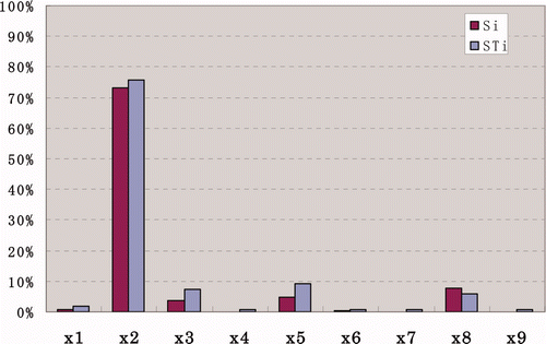
In addition, it is found that X ₃ (cooler wall temperature), X ₅ (Nusselt number in the mixed convection flow regime) and X ₈ (friction factor in the mixed convection flow regime) have small impact on the uncertainty of Y ₁. As far as X ₃ is concerned, it is known from Equation (41) that the variation of the cooler wall temperature will affect the helium gas temperature in the loop. In particular, if the heat flux is constant, the increase of the cooler wall temperature will lead to an increase in the helium gas temperature in the core channels.

Nusselt numbers are directly related to heat transfer coefficients:

where h is the convective heat transfer coefficient (W/(m² K), L is characteristic length (m), and λ is the thermal conductivity of helium gas (W/(m K). Suppose that the cooler wall temperature does not change, if the heat transfer coefficient in the cooler decreases, there will be a decrease in the heat flux in the cooler, which will result in an increase in the helium gas temperature. Suppose that the heat flux in the reactor core does not change, if the heat transfer coefficient in the reactor core decreases, the channel wall temperature will increase, which will also lead to an increase in the helium gas temperature. The reasons that the Nusselt number in the mixed convection flow regime (X ₅) is more important than that in the forced convection flow regime (X ₄) and that in the free convection flow regime (X ₆) can be explained from two aspects. One main reason is that the helium gas flow works mainly in the mixed convection flow regime in the reactor core and the HX [11]. The other reason is that the uncertainty of the parameter X ₅ itself is larger than those of X ₄ and X ₆ because the mixed convection correlations are not supported by extensive experimental results [7].

As to friction factors, it is known from Equation (42) that friction factors affect the pressure losses, which further affects the natural circulation flow rate. If there is an increase in the friction factor, there will be an increase in the pressure losses along the closed loop, which will result in a decrease in the helium gas flow rate. On the contrary, small friction factors will result in an increase in the helium gas flow rate. This flow rate will directly affect the heat flux in the close loop and further affects the helium gas temperature in the heater and the cooler (see Equation (41)). If the helium gas flow rate is low, its temperature will increase. The reasons that the friction factor in the mixed convection flow regime (X ₈) is more important than the Nusselt number in the forced convection flow regime (X ₇) and that in the free convection flow regime (X ₉) are the same as those explanations for X ₅.

It is known from Table 3 that, when the effect of each input parameter is taken alone, 3.8%, 4.9%, and 7.6% of the uncertainty in Y ₁ is attributed to X ₃, X ₅, and X ₈, individually. These proportions will increase to 4.5%, 5.7%, and 9.2%, respectively, when the interaction of each of these three parameters (X ₃, X ₅, and X ₈) with other input parameters is considered. Either based on S_i or S_Ti , we know that X ₈ has the second most important impact on the uncertainty of Y ₁, followed by X ₅ and X ₃. Because friction factors are associated to coolant flow rates and Nusselt numbers are associated to heat transfer coefficients, we can infer that, in the hot channel, the uncertainty in the helium gas flow rate has stronger impact on the helium gas temperature than the heat transfer coefficient has.

5.3. Ranking of parameters contributing to the uncertainty in Y₂

The contribution ratios of the input parameters to the uncertainty of Y ₂ are summarized in Table 4 and are plotted in Figure 5. Similar to the results in Table 3, the system pressure X ₂ is still the most important parameter affecting the uncertainty of Y ₂. It contributes to 72.4% of the uncertainty of Y ₂ when it is considered alone. If the interactions of X ₂ with other input parameters are taken into account, its total contribution to the uncertainty of Y ₂ will increase to 75.8%. In addition, X ₃, X ₅, and X ₈ also have small impact on the uncertainty of Y ₂, which contribute 7.2%, 8.3%, and 4.8% of the uncertainty of Y ₂ individually when each of them is taken alone. Even when the interaction of these parameters with other input parameters is considered, their contributions only increase a little, which are 0.2%, 0.9%, and 1%, respectively. For Y ₂, X ₅ has more impact on its uncertainty than X ₈ has, which means that the uncertainty in the heat transfer coefficient contributes more to the uncertainty in the helium gas temperature in the average channel than the uncertainty in the helium gas flow rate does.

Table 4. Contributions of uncertain input parameters to the uncertainty of the model output Y ₂.

Parameter	Contributions to the uncertainty of Y 1 based on Si (%)		Contributions to the uncertainty of Y 2 based on STi (%)
	Ratio	Ranking	Ratio	Ranking
X 1 (core power)	0.93%	5	1.7%	5
X 2 (system pressure)	72.4%	1	75.8%	1
X 3 (cooler wall temperature)	7.2%	3	7.4%	3
X 4 (Nu number, forced)	0.007%	7	0.9%	6
X 5 (Nu number, mixed)	8.3%	2	9.2%	2
X 6 (Nu number, free)	0.1%	6	0.9%	8
X 7 (friction factor, forced)	0.004%	8	0.9%	9
X 8 (friction factor, mixed)	4.8%	4	5.8%	4
X 9 (friction factor, free)	0.003%	9	0.9%	7

Figure 5. The contribution ratios of the nine uncertain input parameters to the uncertainty of the helium gas temperature at the outlet of the average channel.

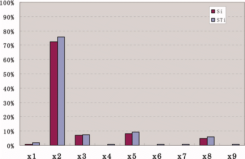
It is noticed that while the friction factor X ₈ ranks the second important parameter with regard to the uncertainty of Y ₁, it ranks the fourth with regard to the uncertainty of Y ₂. This ranking difference can be explained as follows. Since the helium gas flow rate is low under natural circulation, the flow in the core channels is in the laminar regime [11], where the friction factor is inversely proportional to the Reynolds number and thus strongly dependent on kinematic viscosity. Kinematic viscosity increases exponentially with temperature, which is roughly a function of T^3/2 (T represents temperature) [7]. Because temperature in the hot channel is higher than that in the average channel, there will be a larger change of the friction factor despite a small variation of the helium gas temperature in the hot channel. This will affect the flow rate strongly, leading to a large variation of the helium gas temperature in the hot channel.

For the other five input parameters X ₁, X ₄, X ₆, X ₇, and X ₉, each of them contributes little to the uncertainties in Y ₁ and Y ₂ (no more than 1% when each of them is taken alone, and no more than 2% when its interactions with other input parameters are considered. Therefore, the uncertainties of these parameters are comparatively negligible.

6. Conclusions

Passive systems are now of interest to the design of future generation nuclear reactors because it can avoid the failure of active components (e.g., pumps) and reduction of human error. On the other hand, the uncertainties associated with passive systems are usually larger than those in active systems, due to lack of data on a full spectrum of the phenomena a passive system might occur during its lifetime and due to limited experience in operating these systems. This work contributes to the uncertainty study of passive systems. The subject of this work is a natural convection decay heat removal system of a GFR. A simplified steady-state model of this system under a post-LOCA condition was analyzed by variance-based sensitivity analysis methods for identifying the important factors contributing to the uncertainties in the model outputs. The results show that the system pressure has the most important impact on the variations of the helium gas temperatures at the core channel outlets. The strong sensitivity of the helium gas temperature to the system pressure shows that it is critical to reduce the variation of this pressure to achieve a stable system performance. In addition to the pressure level in the guard containment, the system pressure in the post-LOCA conditions is also affected by the energy stored in the system before the accident, the dynamics of the accident. These should be carefully considered when designing this system.

In addition, the Nusselt number and the friction factor in the mixed flow regime as well as the wall temperature of the HX were also found to have small impacts on the helium gas temperatures. This is because the helium coolant works mainly in mixed convection flow regimes in the systems. However, the impact of these two parameters on the variation of the helium gas temperature is much smaller than the system pressure has. The reduction of the uncertainty associated with the Nusselt number and the friction faction in the mixed convection flow regime depends on better modeling the phenomena in this flow regime. This needs much more input from basic research and therefore is difficult. Careful design of the system to transfer the flow regime of the working fluid from the mixed flow regime to the forced flow regime might be considered if the impact of these two parameters on the system performance is to be reduced further.

The wall temperature of the HX was also found to have a small impact on the variation of the helium temperature. To reduce this impact, the secondary side of the HX (water is the proposed secondary side coolant) needs to be carefully designed with the consideration of the change of inlet water temperature which is affected by the ambient conditions. In addition, the fouling of the pipe surface will also affect heat transfer and further affect the performance of the entire system.

Acknowledgements

Part of this work was done when the first author visited MIT Department of Nuclear Science and Engineering. The first author thanks Prof. George Apostolakis, Nicola Pedroni, and Dustin Langewisch for fruitful discussions. The authors also thank the anonymous referee for their valuable comments which have led to an improved work. The views expressed in this work are the authors only and do not represent any others.

References

- Burgazzi , L. 2003 . Reliability evaluation of passive systems through functional reliability assessment . Nucl. Technol , 144 : 145 – 151 .
- Burgazzi , L. 2004 . Evaluation of uncertainties related to passive systems performance . Nucl. Eng. Des , 230 : 93 – 106 .
- Jafari , J. , Auria , F. , Kazeminejad , H. and Davilu , H. 2003 . Reliability evaluation of a natural circulation system . Nucl. Eng. Des , 224 : 79 – 104 .
- Pagani , L.P. , Apostolakis , G.E. and Hejzlar , P. 2005 . The impact of uncertainties on the performance of passive systems . Nucl. Technol , 149 : 129 – 140 .
- Zio , E. and Pedroni , N. 2009 . Estimation of the functional failure probability of a thermal-hydraulic passive system by subset simulation . Nucl. Eng. Des , 239 : 580 – 599 .
- Zio , E. and Pedroni , N. 2009 . Functional failure analysis of a thermal-hydraulic passive system by means of line sampling . Reliab. Eng. Syst. Saf , 94 : 1764 – 1781 .
- Hejzlar , P. 2001 . A modular gas turbine fast reactor concept (MFGR-GT) . Trans. Am. Nucl. Soc , 84
- Okano , Y. , Hejzlar , P. and Driscoll , M.J. 2002 . Thermal hydraulics and shutdown cooling of supercritical CO2 GT-GCFRs , MIT Department of Nuclear Engineering . MIT-ANP-TR-088
- Eapen , J. , Hejzlar , P. and Driscoll , M.J. 2002 . Analysis of a natural convection loop for post-LOCA GCFR decay heat removal , MIT Department of Nuclear Engineering . MIT-GCFR-002
- Williams , W. , Hejzlar , P. , Driscoll , M.J. , Lee , W.J. and Saha , P. 2003 . Analysis of a convection loop for GFR post-LOCA decay heal removal from a block-type core , MIT Department of Nuclear Engineering . MIT-ANP-TR-095
- Williams , W.C. , Hejzlar , P. and Saha , P. 2004 . Analysis of a Convection Loop for GFR Post-LOCA Decay Heat Removal . Proceedings of ICONE 12 . April 25–29 2004 .
- Hora , S.C. and Iman , R.L. 1986 . A comparison of maximum/bounding and Bayesian/Monte Carlo for fault tree uncertainty analysis , Sandia National Laboratories . SAND85-2839
- Iman , R.L. 1987 . A matrix-based approach to uncertainty and sensitivity analysis for fault trees . Risk Anal , 7 : 21 – 33 .
- Sobol , I.M. 1993 . Sensitivity estimates for nonlinear mathematical models . Math. Model. Comput. Exp , 1 : 407 – 414 .
- Homma , T. and Saltelli , A. 1996 . Importance measures in global sensitivity analysis of nonlinear models . Reliab. Eng. Syst. Saf , 52 : 1 – 17 .
- Borgonovo , E. 2007 . A new uncertainty importance measure . Reliab. Eng. Syst. Saf , 92 : 771 – 784 .
- Liu , Q. and Homma , T. 2010 . A new importance measure for sensitivity analysis . J. Nucl. Sci. Technol , 47 : 53 – 61 .
- Saltelli , A. , Tarantola , S. and Campolongo , F. 2000 . Sensitivity analysis as an ingredient of modelling . Stat. Sci , 15 : 377 – 395 .
- Rabitz , H. , Ali , O.F. , Shorter , J. and Shim , K. 1999 . Efficient input–output model representations . Comput. Phys. Commun , 117 : 11 – 20 .
- Saltelli , A. , Chan , K. and Scott , E.M. 2000 . Sensitivity Analysis , Chichester : John Wiley & Sons . ISBN 0471998923
- Cukier , R.L. , Fortuin , C.M. , Shuler , K.E. , Petschek , A.G. and Schaibly , J.H. 1973 . Study of the sensitivity of coupled reaction systems to uncertainties in rate coefficients. I: Theory . J. Chem. Phys , 59 : 3873 – 3878 .
- Schaibly , J.H. and Shuler , K.E. 1973 . Study of the sensitivity of coupled reaction systems to uncertainties in rate coefficients. II: Applications . J. Chem. Phys , 59 : 3979 – 3888 .
- Cukier , R.I. , Schaibly , J.H. and Shuler , K.E. 1975 . Study of the sensitivity of couples reaction systems to uncertainties in rate coefficients. III: Analysis of the approximations . J. Chem. Phys , 63 : 1140 – 1149 .
- Cukier , R.I. , Levine , H.B. and Shuler , K.E. 1978 . Nonlinear sensitivity analysis of multiparameter model systems . J. Comput. Phys , 26 : 1 – 42 .
- Saltelli , Tarantola , S. and Chan , K. 1999 . A quantitative model-independent method for global sensitivity analysis of model output . Technometrics , 41 : 39 – 56 .
- Zio , E. and Apostolakis , G.E. 1996 . Two methods for the structured assessment of model uncertainty by experts in performance assessment in radioactive waste repositories . Reliab. Eng. Syst. Saf , 54 : 225 – 241 .
- Churchill , S.W. 1998 . “ Combined free and forced convection in channels ” . In Heat Exchanger Design Handbook , Edited by: Hewitt , G.F. New York : Begell House . Sec. 2.5.10
- Gnielisnki , V. New equations for heat and mass transfer in turbulent pipe and channel flow . Int. Chem. Eng , 16 359 – 368 .
- Liu , Q. , Homma , T. , Nishimaki , Y. , Hayashi , H. , Terakado , M. and Tamura , S. 2010 . GSALab computer code for global sensitivity analysis , Japan Atomic Energy Agency . JAEA-Data/Code 2010-001