Source term estimation of atmospheric release due to the Fukushima Dai-ichi Nuclear Power Plant accident by atmospheric and oceanic dispersion simulations

Abstract

The source term of the atmospheric release of ¹³¹I and ¹³⁷Cs due to the Fukushima Dai-ichi Nuclear Power Plant accident estimated by previous studies was validated and refined by coupling atmospheric and oceanic dispersion simulations with observed ¹³⁴Cs in seawater collected from the Pacific Ocean. By assuming the same release rate for ¹³⁴Cs and ¹³⁷Cs, the sea surface concentration of ¹³⁴Cs was calculated using the previously estimated source term and was compared with measurement data. The release rate of ¹³⁷Cs was refined to reduce underestimation of measurements, which resulted in a larger value than that previously estimated. In addition, the release rate of ¹³¹I was refined to follow the radioactivity ratio of ¹³⁷Cs. As a result, the total amounts of ¹³¹I and ¹³⁷Cs discharged into the atmosphere from 5 JST on March 12 to 0 JST on March 20 were estimated to be approximately 2.0 × 10¹⁷ and 1.3 × 10¹⁶ Bq, respectively.

Keywords:

• release amounts
• ¹³¹I
• ¹³⁷Cs
• atmosphere
• ocean
• Fukushima Dai-ichi nuclear power plant
• monitoring data
• dispersion simulation
• WSPEEDI-II
• SEA-GEARN

View correction statement:

Corrigendum

CORRIGENDUM

1. Introduction

A large amount of radionuclides was discharged into the atmosphere by the Fukushima Dai-ichi Nuclear Power Plant (FNPP1) accident in Japan, which was caused by the great east Japan earthquake and tsunami on March 11, 2011. The radionuclides released from the FNPP1 were transferred eastward by a strong jet stream and reached the west coast of North America within four days [1]. A portion of the airborne radionuclides was deposited into the Pacific Ocean by a dry/wet deposition process. Moreover, water used to cool a damaged nuclear reactor leaked into the ocean. Tokyo Electric Power Company (TEPCO) estimated that 4.7 × 10¹⁵ Bq of radioactive materials including ¹³¹I, ¹³⁴Cs, and ¹³⁷Cs were released directly into the ocean from a pit of the Unit 2 reactor during April 1–6, 2011 [2]. In addition, TEPCO confirmed the following accidental/intentional direct releases into the ocean: (1) an intentional discharge of 1.5 × 10¹¹ Bq of low-level wastewater during April 4–10, (2) an accidental release estimated at 2.0 × 10¹³ Bq from the Unit 3 reactor on May 11, and (3) an accidental leakage of 2.6 × 10¹⁰ Bq from a desalination plant on December 4.

Assessment of the accident's influence on the marine environment should include a fundamental understanding of the actual conditions of radionuclide release into the ocean through direct and atmospheric pathways. Numerical simulations of radionuclide migration near the coastal region attributed to the FNPP1 accident have been performed by several authors [3–6]. In addition, long-term climatological simulation models that include 10–30 year forecasting results for the entire Pacific region have been reported [7,8]. These studies performed atmospheric dispersion simulations of the radionuclide release into the ocean through the atmospheric pathway on the basis of the source term estimated by previous studies [9–12]. However, it should be noted that while the source term for the period in which the plume flowed over land in Japan is reasonable, that for the period in which the plume flowed into and deposited over the ocean could not be verified [12]. Therefore, it is important to validate the source term of atmospheric release through measurements of the seawater collected from the Pacific Ocean.

In this study, as a first step toward a better understanding of radionuclide dispersion in the Pacific Ocean due to the FNPP1 accident, the source term of atmospheric release estimated by a previous study [12] was validated by coupling atmospheric and oceanic dispersion simulations with ¹³⁴Cs observed in the seawater collected from the Pacific Ocean.

The oceanic dispersion of ¹³⁴Cs has been simulated using ¹³⁴Cs deposition on the sea surface calculated by an atmospheric dispersion model. The source term of ¹³⁴Cs was given by that determined by Terada et al. [12], hereafter the initial source term, by assuming the same release rate for ¹³⁴Cs and ¹³⁷Cs. The simulation results obtained using the initial source term showed good agreement with most observed sea surface concentration of ¹³⁴Cs. However, the simulation results for the eastern North Pacific showed a tendency of underestimating observed sea surface concentration of ¹³⁴Cs. We believed that this tendency resulted from an underestimation of the initial source term. Therefore, the source term of the atmospheric release of radionuclides, hereafter the new source term, was refined to reduce the underestimation of observed sea surface concentration of ¹³⁴Cs collected from the Pacific Ocean. This refinement of the source term is a first effort to feed oceanic dispersion analysis results back into atmospheric dispersion analysis.

In Section 2, we describe the four models and discuss the validation results of the initial source term and the estimation method for the new source term from observed ¹³⁴Cs in seawater. In Section 3, the results of the new source term and simulation of ¹³⁴Cs using the new source term are explained.

2. Methods

2.1. Numerical models for atmospheric dispersion

The Worldwide Version of System for Prediction of Environmental Emergency Dose Information (WSPEEDI-II) [13] was used to simulate the atmospheric dispersion of radionuclides released from the FNPP1 over the Pacific Ocean. WSPEEDI-II calculates air concentration and the surface deposition of radionuclides and radiological doses using the nonhydrostatic mesoscale meteorological prediction model (MM5) [14] and the Lagrangian particle dispersion model (GEARN) [15]. Concerning deposition processes for radiocesium in GEARN, the deposition velocity was set at a constant of 1 mm s⁻¹ [10]; the amount of wet deposition of each particle was proportional to its radioactivity with the scavenging coefficient Λ s⁻¹ calculated from the precipitation intensity γ mm h⁻¹ with Λ = αγ^β. The constants α and β were set at 5.0 × 10⁻⁵ and 0.8, respectively [12].

The calculation period of WSPEEDI-II was from 5 JST (UTC + 9 h) on March 12 to 0 JST on May 1. The computational domain includes the entire North Pacific region (Figure 1) with a horizontal resolution of 80 km. In the vertical resolutions, 23 sigma levels from the surface to 100 hPa and 20 levels from the surface (with a bottom layer of 20 m thickness) to 10 km were set in MM5 and GEARN, respectively. The radioactivity ratio of ¹³⁴Cs/¹³⁷Cs was assumed to be 1.0 [16]; therefore, we also treated the release rate of ¹³⁴Cs to be the same as that of ¹³⁷Cs in this study. Thus, the source term of ¹³⁴Cs was given by the initial source term of ¹³⁷Cs in Terada et al. [12]. The calculated deposition amounts were given to the Lagrangian oceanic particle dispersion model (SEA-GEARN) every 24 h. Further details of WSPEEDI-II and its prediction performance are described in Terada et al. [15].

Figure 1 Simulation area and locations of the sampling stations used for verification and refinement of the source term of atmospheric release from the Fukushima Dai-ichi Nuclear Power Plant (FNPP1). Circles (triangles) on the map indicate calculations within (without) a factor of 10 of the measurements in Figure 3. Crosses on the map indicate that ¹³⁴Cs released directly into the ocean from the FNPP1 may have an influence on the ¹³⁴Cs concentration in surface water, as indicated by a preliminary modeling study. Numbers with the prefix “J” indicate the sampling points reported by Honda et al. [22], and those without the prefix “J” indicate the sampling points reported by the Meteorological Research Institute [23]

2.2. Numerical models for oceanic dispersion

SEA-GEARN used the 10-day mean ocean current, simulated by the coupled ocean–atmosphere global model K7 [17], as an input variable. K7 is a fully coupled global general circulation model (GCM) developed by Data Research Center for Marine–Earth Sciences, Japan Agency for Marine–Earth Science and Technology (JAMSTEC/DrC). The coupled GCM is composed of the Atmospheric GCM for the Earth Simulator (AFES) [18] and the Ocean–Sea Ice GCM for the Earth Simulator (OIFES) [19]. The resolution of the AFES component is T42 horizontally (approximately 2.8°) and 24 layers in vertical σ coordinates. The resolution of the OIFES component is 1° horizontally and 45 vertical layers. The four-dimensional variation method, one of the highly efficient data assimilation techniques, was used to execute reanalysis data in K7.

The assimilated elements for the OIFES included temperature and salinity from the Fleet Numerical Meteorology and Oceanography Center (FNMOC) dataset, sea surface temperature from OISST version 2, sea surface dynamic height anomaly data from TOPEX/Poseidon altimetry, and the monthly mean temperature and salinity field of the World Ocean Database 2001 (WOD2001). The assimilated elements for the AFES included air temperature, specific humidity, and wind vector from National Oceanic and Atmospheric Administration/National Centers for Environmental Prediction (NOAA/NCEP). Further details of K7 and its prediction performance are described in Sugiura et al. [17]. The optimization of the initial value of OIFES and sea surface bulk correction coefficients, including the coefficients of each bulk formula of latent heat, sensible heat, and momentum flux, were iterated to approach the observed dataset during the reanalysis period from January 1 to June 30.

SEA-GEARN is a particle random-walk model to simulate radionuclide transport in oceans [20]. Cesium-134 (half life = 2.1 years) was considered in the calculation. The computational domain includes the entire North Pacific region (Figure 1). The horizontal and vertical resolutions are same as those of OIFES in K7. Turbulent mixing was modeled using the Smagorinsky formula [21] for horizontal fluxes. For vertical fluxes, the average for the mixed layer of an entire calculation period of K7, namely 4 × 10⁻³ m² s⁻¹, was used for the entire model grid. The time step was 20 min. The calculation period of SEA-GEARN was from March 12 to June 30.

The source term of radionuclides released directly into the ocean from the FNPP1 was estimated by modifying the release period (from March 21 to April 30) given by Kawamura et al. [4]. In particular, analysis of the ¹³¹I/¹³⁷Cs activity ratio [3] indicated that the direct release into the ocean began on March 26 and was extended up to June 30. As a result of the above modification, the total amount of direct release into the ocean from March 26 to June 30 was estimated to be approximately 1.1 × 10¹⁶ Bq for ¹³¹I and 3.5 × 10¹⁵ Bq for ¹³⁷Cs. Because the monitoring data of ¹³¹I near the FNPP1 became less than the detection limit on and after May 30, the release period of ¹³¹I became shorter, from March 26 to May 29, than that of radioactive cesium.

2.3. Measurement data for the ocean used for the estimation of the new source term

Imprints of former atmospheric nuclear tests were detected in the seawater sample of ¹³⁷Cs. Thus, ¹³⁴Cs was adopted for the estimation of the new source term. ¹³⁴Cs measured in the seawater used for the estimation was observed by Honda et al. [22] and the Meteorological Research Institute, Japan (MRI) [23]. We used SEA-GEARN to perform a preliminary simulation that only considered the direct release from the FNPP1 into the ocean and excluded atmospheric deposition on the sea surface. Sampling points that could have been influenced by direct release from the FNPP1, indicated by crosses on the map shown in Figure 1, as well as those below detection limits were excluded from the new source term estimation. Thus, the measurement data of 54 points were used for the estimation of the new source term during observation periods of April 14–May 3, 2011 for Honda et al. [22] and March 31–May 17, 2011 for MRI [23].

2.4. Validation of the source term by ¹³⁴Cs simulation

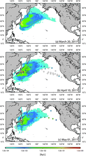
The horizontal distribution of the sea surface concentration of ¹³⁴Cs used for calculation with the initial source term and for measurements obtained during March 31–May 17 is shown in Figure 2. Because a coarse resolution of the horizontal grid space was used in the calculation, the results of the surface concentration of radionuclides close to the Japanese coast that are reported in Kawamura et al. [4] are not detailed in the present study. An image of the horizontal distribution recorded on March 20 (Figure 2(a)) shows that ¹³⁴Cs was deposited on the sea surface along Fukushima and Miyagi prefectures and in the offshore area northeast and southeast of the FNPP1. Less than 1 × 10⁻³ Bq L⁻¹ of ¹³⁴Cs, a substantially low amount, reached the coastal area of California, USA and the Bering Sea. One to two months after the FNPP1 accident (Figure 2 (b) and (c)), approximately 1 × 10⁻³ Bq L⁻¹ of ¹³⁴Cs was reported near Japan in areas such as the Okhotsk Sea and Japan Sea. Thus, the FNPP1 accident widely dispersed radionuclides across the entire North Pacific region.

Figure 2 Horizontal distribution of sea surface ¹³⁴Cs obtained by simulation with the initial source term on (a) March 20, (b) April 10, and (c) May 1. Colors of circles in the figures represent observed sea surface concentration of ¹³⁴Cs at sampling points (b) from March 31 to April 18 and (c) from April 21 to May 17, 2011

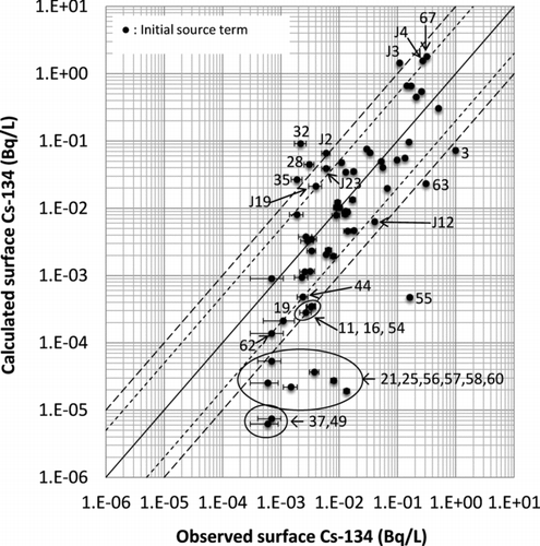
The results of a comparison between the simulation and measurements of the sea surface concentration of ¹³⁴Cs and statistics on the percentage of calculations of sea surface concentration of ¹³⁴Cs that are within factors of 2, 5, and 10 of the measurements are plotted in Figure 3 and summarized in Table 1, respectively. The simulation results using the initial source term showed good agreement with observed data (Figure 3) with an FA10 of 75% (Table 1). However, simulation results in some area of the eastern North Pacific (Nos. 21, 25, 37, 49, 55−58, and 60 in Figure 3) showed a tendency of underestimation against observed data. The horizontal distribution of the sea surface concentration of ¹³⁴Cs in Figure 2 indicates that the simulation results in the eastern North Pacific were also lower than the measurement results. This tendency indicates that the actual abundance of ¹³⁴Cs in the eastern North Pacific was higher than that obtained by calculation using the initial source term. We attributed this tendency to an underestimation of the release rate in the initial source term for some periods. The initial source term was estimated on the basis of environmental monitoring data on land. However, monitoring data in the ocean were not considered. Therefore, the source term of the atmospheric release of radionuclides, hereafter the new source term, was refined using ¹³⁴Cs observed in the seawater collected from the North Pacific.

Table 1 Statistics of sea surface concentration of ¹³⁴Cs calculated from data points between March 31 and May 17, 2011. Values of FA2, FA5, and FA10 denote the percentage of calculations within factors of 2, 5, and 10 of the measurements, respectively

Release rate used for calculations	FA2 (%)	FA5 (%)	FA10 (%)	Correlation coefficients
Initial source term	35	60	75	0.54
New source term	37	65	77	0.53

Figure 3 Scatter diagram of the sea surface concentration of ¹³⁴Cs comparing measurements and calculations using the initial source term. Solid lines show 1:1 lines, and the areas between two long-dashed (short-dashed) lines indicate the bands within a factor of 10 (5). The numbers in the figure denote the sampling points shown in Figure 1

2.5. Estimation of the new source term

We set the estimation period as March 12–20 to reflect the large release rate change reported by previous studies [10,12]. The release period was separated into 18 terms, as shown in Figure 4. Numbers with the prefix “a” in the figure indicate a period in which the release rates were determined on the basis of land monitoring data [9,10]. We estimated the new release rate during these periods. No land monitoring data was available; therefore, the hydrogen explosion at Unit 3 was assumed to be the same as the explosions at Unit 1 in the initial source term [12]. For this reason, the Unit 3 event was time-averaged to “term 5” for estimation using measurement data in the ocean.

Figure 4 Time variation of estimated new release rates of ¹³¹I and ¹³⁷Cs from March 12 to 20, 2011. Dotted lines show the initial release rates reported by Terada et al. [12]. Divided periods of estimation are represented by gray lines. The date and time of important plant events are also shown in figure. This figure is modified from Figure 4 of Katata et al. [10]

The new release rates at each term were estimated by the following method. First, two model simulations were conducted to calculate the sea surface concentration of ¹³⁴Cs. These included atmospheric dispersion simulation by GEARN that used the initial release rate, followed by oceanic dispersion simulation by SEA-GEARN that used sources such as direct release from the FNPP1 into the ocean and atmospheric deposition derived from the simulation of GEARN. The correction coefficient for the initial source term, which assumed that these dispersion simulations are correct, was obtained by measuring the calculated sea surface concentration of ¹³⁴Cs at the sampling point i as follows:

where R_i is the correction coefficient at the sampling point i, M_i is the measured sea surface concentration (Bq L⁻¹) of ¹³⁴Cs at the sampling point i, and C_i is the calculated sea surface concentration (Bq L⁻¹) of ¹³⁴Cs at the sampling point i at 12 JST on the same observed date. The range of R _i was 0.024 to 706.

Next, to investigate the correction quantity on the basis of the cumulative deposition amount, i.e., to estimate which release period should be corrected, the contribution of deposition must be measured for each release period at each sampling point. In particular, unit release (1 Bq h⁻¹) calculations during each of the 18 terms of the release periods shown in Figure 4 were performed by GEARN. The daily deposition data of each simulation result were used as the input in the calculation of SEA-GEARN. The direct release from the FNPP1 into the ocean was not considered in the calculation of SEA-GEARN. The sea surface concentration D_ij (Bq L⁻¹) of ¹³⁴Cs at the sampling point i at 12 JST on the same observed date were extracted from the calculation results of each term. A large D_ij indicates that the term j at the sampling point i has a large contribution to the deposition. The contribution at each term j and sampling point i are obtained by considering the initial source term as follows:

where IRate_j is the initial release rate (Bq h⁻¹) at term j, which was estimated by Terada et al. [12]. As a result, the contribution ratio at each term j to the sum of all terms at the sampling point i is written as follows:

The correction coefficient X_j , which considers the weighting of the contribution ratio at each sampling point i, is written as

Finally, in this study, the new release rate NRate_j (Bq h⁻¹) at term j is written by multiplying IRate_j with the rate X_j :

3. Results

3.1. Estimation results for the new source term

The new release rate of ¹³⁷Cs was derived from that of ¹³⁴Cs because the assumed radioactivity ratio of ¹³⁴Cs/¹³⁷Cs is 1.0. The radioactivity ratio of ¹³¹I/¹³⁷Cs determined by Terada et al. [12] was also used for estimating the new release rate of ¹³¹I. The time variation and values of the new source terms of ¹³¹I and ¹³⁷Cs are shown in Table 2 . These time variations are compared with the initial release rate in Figure 4. For estimating the new release rate, a coarse oceanographic model of 1° horizontal resolution was used; therefore, a sharp change in the release rate could not be expressed.

Table 2 Release period, release duration, release rates of ¹³⁷Cs and ¹³¹I, and rate X_j , shown in Equation (4), for the period between 5 JST on March 12 and 0 JST on March 20

No. of release	Release period	Release	Release rate	Release rate	Xj in
period in Fig.4	(month/day time JST)	duration (h)	of ^137Cs (Bq h^-1)	of ^131I (Bq h^-1)	eq. (4)
a1	3/12 05:00-3/12 09:30	4.5	1.1E+13	1.1E+14	3.0
a1	3/12 09:30-3/12 15:30	6	5.0E+12	5.0E+13	3.0
a1	3/12 15:30-3/12 16:00	0.5	8.9E+14	8.9E+15	3.0
1	3/12 16:00-3/13 00:00	8	2.3E+13	2.3E+14	2.7
2	3/13 00:00-3/13 11:00	11	2.8E+13	2.8E+14	3.3
a2	3/13 11:00-3/13 15:00	4	3.3E+13	3.3E+14	3.9
3	3/13 15:00-3/13 23:00	8	3.7E+13	3.7E+14	4.4
4	3/13 23:00-3/14 11:00	12	1.1E+13	1.1E+14	3.1
5	3/14 11:00-3/14 19:00	8	2.5E+13	2.5E+14	1.2
a3	3/14 19:00-3/14 21:30	2.5	4.2E+12	4.2E+13	1.8
a3	3/14 21:30-3/15 00:00	2.5	2.4E+14	2.4E+15	1.8
a3	3/15 00:00-3/15 07:00	7	7.3E+13	6.4E+14	1.8
a3	3/15 07:00-3/15 10:00	3	5.5E+14	5.5E+15	1.8
a3	3/15 10:00-3/15 13:00	3	1.5E+13	1.5E+14	1.8
a3	3/15 13:00-3/15 17:00	4	7.3E+14	7.3E+15	1.8
6	3/15 17:00-3/16 02:00	9	1.2E+13	8.3E+14	3.9
a4	3/16 02:00-3/16 06:00	4	9.9E+12	6.9E+14	3.3
7	3/16 06:00-3/16 18:00	12	5.5E+12	3.8E+14	1.8
8	3/16 18:00-3/17 06:00	12	8.2E+12	5.8E+14	2.7
9	3/17 06:00-3/17 18:00	12	1.2E+13	5.0E+14	1.2
10	3/17 18:00-3/18 06:00	12	1.1E+13	4.6E+14	1.1
a5	3/18 06:00-3/18 10:00	4	2.3E+13	9.5E+14	2.3
11	3/18 10:00-3/19 00:00	14	3.1E+13	1.3E+15	3.1
12	3/19 00:00-3/19 15:00	15	3.0E+13	1.2E+15	3.0
13	3/19 15:00-3/20 00:00	9	4.1E+13	4.5E+14	1.2

The correction coefficient X_j exceeded one in all periods. The lowest value was 1.1 at term 10, from 18 JST on March 17 to 6 JST on March 18, and the highest value was 4.4 at term 3, from 15 to 23 JST on March 13; the average value was 2.5.

The new release rate of ¹³⁷Cs reached the peak of 8.9 × 10¹⁴ Bq h⁻¹ at the term of the hydrogen explosion in Unit 1, from 15:30 to 16 JST on March 12, and dropped to 2.3 × 10¹³ Bq h⁻¹ at term 1, from 16 JST on March 12 to 0 JST on March 13. The rate increased gradually with time to reach 3.7 × 10¹³ Bq h⁻¹ at term 3, from 15 to 23 JST on March 13. Because the plume mainly flowed to the Pacific Ocean owing to a southwesterly–westerly wind from 12 JST on March 12 to 12 JST on March 14 [10], the estimation accuracy of the initial source term at this period was low. Therefore, the estimation method that used observed seawater data gave a more reliable result.

At term 5, from 11 to 19 JST on March 14, the total estimation was 2.0 × 10¹⁴ Bq during the period in which the release rate of the hydrogen explosion in Unit 3 was time-averaged. However, it was impossible to classify the volume of the amount released as a result of this explosion.

The temporal change of the release rate for term a3, from 19 JST on March 14 to 17 JST on March 15, was estimated in detail by previous investigations [9,10]. However, only air dose rates were available as measurements; the release rates of major radionuclides were determined through reproduction of the air dose rates from groundshine by assuming the radioactivity ratio of the radionuclides. The new release rate was 1.8 times larger than the initial release rate. Thus, atmospheric dispersion simulation with the new release rate will result in overestimation of the surface deposition concentration. The contribution of the wet deposition according to rain or snow coverage at this accident is high. Then, for atmospheric dispersion simulation, increasing the wet deposition intensity by approximately 0.6 corrects the new estimation, and the surface deposition concentration would be in agreement with the land monitoring data. However, when the wet deposition intensity is 0.6 times, the sea surface concentration may be underestimated again. Moreover, considering the overestimation of ¹³⁷Cs deposition on the land near the northern part of Japan reported by Terada et al. [12] compared with airborne monitoring, it is expected that the atmospheric dispersion calculation with the initial release rate for this period could reproduce the measurements of ¹³⁴Cs in sea water by reducing the error in deposition prediction. The appropriate source term is obtained by conducting sensitivity analysis of the parameter of wet deposition intensity and repeating the same work as reported in this study by using model simulation and the observed sea surface concentration.

The total amounts of ¹³¹I and ¹³⁷Cs discharged into the atmosphere from 5 JST on March 12 to 0 JST on May 1 are estimated to be approximately 2.0 × 10¹⁷ and 1.3 × 10¹⁶ Bq, respectively.

3.2. Cesium-134 simulation with the new source term

The horizontal distribution of the sea surface concentration of ¹³⁴Cs used for calculation with the new source term and for measurements from March 31 to May 17, 2011 is shown in Figure 5. A comparison of Figure 5 with Figure 2 reveals that the simulation results with the new source term increased the traffic transport of radionuclides to the east. As shown in Figure 5 (b) and (c), the extension of a green contour area of approximately 1 × 10⁻² Bq L⁻¹ northeast of the FNPP1 agrees with the observed data. Figure 6 shows the results of comparison between the simulation and measurements of the sea surface concentration of ¹³⁴Cs using the new source term. The results obtained with the initial source term are also plotted for comparison. Because all the new release rates at all 18 terms increased, the simulated concentration increased relative to the results obtained with the initial release rate. The statistics on the percentage of calculations of the sea surface concentration of ¹³⁴Cs that are within factors of 2, 5, and 10 of the measurements are summarized in Table 1. All statistic values were improved. A comparison of the statistics obtained with the new source term with those obtained with the initial source term reveals that FA5 increased from 60% to 65%. These results indicate that radionuclides observed in seawater can be actually used for estimating the atmospheric source term of nuclear accidents that occur in coastal areas. However, the simulation results in some areas of the eastern North Pacific remain underestimated (Figure 6). As stated in Section 3.1, verification of the atmospheric deposition process plays an important role in resolving these underestimation issues.

Figure 5 Horizontal distribution of sea surface ¹³⁴Cs by simulation using the new source term on (a) March 20, (b) April 10, and (c) May 1, 2011. Colors of circles represent observed sea surface concentration of ¹³⁴Cs at sampling points (b) from March 31 to April 18 and (c) from April 21 to May 17, 2011

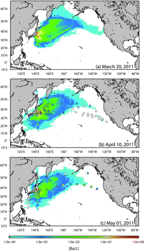
Figure 6 Scatter diagram of the sea surface concentration of ¹³⁴Cs (Bq L⁻¹) comparing measurements and calculations using the initial and new source terms. Solid lines show 1:1 lines, and the areas between two long-dashed (short-dashed) lines indicate the bands within a factor of 10 (5). The numbers in the figure denote the sampling points shown in Figure 1

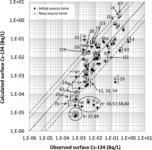
Table 3 summarizes the amounts of ¹³¹I and ¹³⁷Cs that were released into the atmosphere and the ocean and those deposited on the land and ocean surfaces. The deposition amounts of ¹³¹I were 7.4 × 10¹⁶ and 9.9 × 10¹⁶ Bq on the land and ocean surfaces, respectively. For ¹³⁷Cs, the deposition amounts were 5.8 × 10¹⁵ and 7.6 × 10¹⁵ Bq on the land and ocean surfaces, respectively. The results of gross supply to the North Pacific from atmospheric deposition and from direct release from the FNPP1 can be estimated to be 1.1 × 10¹⁷ and 1.1 × 10¹⁶ Bq for ¹³¹I and ¹³⁷Cs, respectively. The new source term of atmospheric and oceanic release offers important information for presuming the remaining radionuclides at the FNPP1.

Table 3 Amounts of ¹³¹I and ¹³⁷Cs released into the atmosphere and ocean and those deposited on land and ocean surfaces (Bq)

		^131I	^137Cs
New source term	Atmosphere (from March 12 to May 1)	2.0 × 10^17	1.3 × 10^16
	Ocean (from March 26 to June 30)	1.1 × 10^16	3.5 × 10^15
Deposition	Land	7.4 × 10^16	5.8 × 10^15
	Ocean	9.9 × 10^16	7.6 × 10^15
Gross supply to the North Pacific		1.1 × 10^17	1.1 × 10^16

4. Summary

The source term of the atmospheric release of radionuclides from the FNPP1 has been refined using observed ¹³⁴Cs in the seawater collected from the Pacific Ocean and four types of numerical models. The results indicated that the release rates of ¹³⁷Cs and ¹³¹I became larger than those previously estimated for most of the period. In addition, total amounts of ¹³¹I and ¹³⁷Cs discharged into the atmosphere from 5 JST on March 12 to 0 JST on May 1 were estimated to be approximately 2.0 × 10¹⁷ and 1.3 × 10¹⁶ Bq, respectively. A comparison of the statistics obtained using the new source term with those obtained with the initial source term showed that all statistic values were improved. This study demonstrated the effectiveness of using radionuclides observed in seawater for estimating the source term of atmospheric release in case of nuclear accidents occurring in coastal areas.

The new source term obtained in this study is a first guess value; therefore, these results contain uncertainty. Various types of models that include physical processes and parameters, resolutions, and regions in addition to environmental data are needed to determine the probable source term. Detailed source term estimation obtained using the coupled atmospheric and oceanic dispersion simulation remains a topic for future research.

Acknowledgements

The authors would like to thank Akiko Furuno for providing the WSPEEDI-II results; Yoichi Ishikawa, Hiromichi Igarashi, and Shiro Nishikawa for providing the K7 results; and Toyokazu Kakefuda for his technical support.

References

- Takemura , T , Nakamura , H , Takigawa , M , Kondo , H , Satomura , T , Miyasaka , T and Nakajima , T . 2011 . A numerical simulation of global transport of atmospheric particles emitted from the Fukushima Daiichi Nuclear Power Plant . SOLA. , 7 : 101 – 104 . doi: 10.2151/sola.2011-026
- 2011 . Report of Japanese government to the IAEA ministerial conference on nuclear safety: The accident at TEPCO's Fukushima Nuclear Power Stations . http://www.kantei.go.jp/foreign/kan/topics/201106/iaea_houkokusho_e.html
- Tsumune , D , Tsubono , T , Aoyama , M and Hirose , K . 2012 . Distribution of oceanic 137Cs from the Fukushima Dai-ichi Nuclear Power Plant simulated numerically by a regional ocean model . J Environ Radioact. , 111 : 100 – 108 . doi:10.1016/j.jenvrad.2011.10.007 doi: 10.1016/j.jenvrad.2011.10.007
- Kawamura , H , Kobayashi , T , Furuno , A , In , T , Ishikawa , Y , Nakayama , T , Shima , S and Awaji , T . 2011 . Preliminary numerical experiments on oceanic dispersion of 131I and 137Cs discharged into the ocean because of Fukushima Daiichi nuclear power plant disaster . J Nucl Sci Technol. , 48 : 1349 – 1356 . doi: 10.1080/18811248.2011.9711826
- Bailly du Bois , P , Laguionie , P , Boust , D , Korsakissok , I , Didier , D and Fiévet , B . 2012 . Estimation of marine source-term following Fukushima Dai-ichi accident . J Environ Radioact. , 114 : 2 – 9 . doi: 10.1016/j.jenvrad.2011.11.015
- Miyazawa , Y , Masumoto , Y , Varlamov , S M and Miyama , T . 2012 . Transport simulation of the radionuclide from the shelf to open ocean around Fukushima . Cont Shelf Res. , doi:10.1016/j.csr.2012.09.002. Forthcoming
- Nakano , M and Povinec , P P . 2011 . Long-term simulations of the 137Cs dispersion from the Fukushima accident in the world ocean . J Environ Radioact. , 111 : 109 – 115 . doi:10.1016/j.jenvrad.2011.12.001 doi: 10.1016/j.jenvrad.2011.12.001
- Behrens , E , Schwarzkopf , F U , Lubbecke , J F and Boning , C W . 2012 . Model simulations on the long-term dispersal of 137Cs released into the Pacific Ocean off Fukushima . Environ Res Lett. , 7 stacks.iop.org/ERL/7/034004 doi: 10.1088/1748-9326/7/3/034004
- Chino , M , Nakayama , H , Nagai , H , Terada , H , Katata , G and Yamazawa , H . 2011 . Preliminary estimation of release amounts of 131I and 137Cs accidentally discharged from the Fukushima Daiichi Nuclear Power Plant into atmosphere . J Nucl Sci Technol. , 48 : 1129 – 1134 . doi: 10.1080/18811248.2011.9711799
- Katata , G , Ota , M , Terada , H , Chino , M and Nagai , H. 2012 . Atmospheric discharge and dispersion of radionuclides during the Fukushima Dai-ichi Nuclear Power Plant accident. Part I: source term estimation and local-scale atmospheric dispersion in early phase of the accident . J Environ Radioact. , 109 : 103 – 113 . doi: 10.1016/j.jenvrad.2012.02.006
- Katata , G , Terada , H , Nagai , H and Chino , M . 2012 . Numerical reconstruction of high dose rate zones due to the Fukushima Dai-ichi Nuclear Power Plant accident . J Environ Radioact. , 111 : 2 – 12 . doi: 10.1016/j.jenvrad.2011.09.011
- Terada , H , Katata , G , Chino , M and Nagai , H. 2012 . Atmospheric discharge and dispersion of radionuclides during the Fukushima Dai-ichi Nuclear Power Plant accident. Part II: verification of the source term and analysis of regional-scale atmospheric dispersion . J Environ Radioact. , 112 : 141 – 154 . doi: 10.1016/j.jenvrad.2012.05.023
- Terada , H , Nagai , H , Furuno , A , Kakefuda , T , Harayama , T and Chno , M . 2008 . Development of worldwide version of system for prediction of environmental emergency dose information: WSPEEDI 2nd version . Trans Atomic Energy Soc. , 7 : 257 – 267 . [in Japanese with English abstract] doi: 10.3327/taesj.J07.045
- Grell , G A , Dudhia , J and Stauffer , D R . 1994 . A description of the fifth-generation Penn State/NCAR Mesoscale Model (MM5) . : 122 NCAR Tech. Note, NCAR/TN-398þSTR
- Terada , H and Chino , M . 2005 . Improvement of Worldwide Version of System for Prediction of Environmental Emergency Dose Information (WSPEEDI), (II) Evaluation of numerical models by 137Cs deposition due to the Chernobyl nuclear accident . J Nucl Sci Technol. , 42 : 651 – 660 . doi: 10.1080/18811248.2004.9726433
- 2011 . MEXT , http://www.mext.go.jp/english/
- Sugiura , N , Awaji , T , Masuda , S , Mochizuki , T , Toyoda , T , Miyama , T , Igarashi , H and Ishikawa , Y . 2008 . Development of a four-dimensional variational coupled data assimilation system for enhanced analysis and prediction of seasonal to interannual climate variations . J Geophys Res. , 113 Jul C10017; doi:10.1029/2008JC004741 doi: 10.1029/2008JC004741
- Ohfuchi , W , Nakamura , H , Yoshioka , M K , Enomoto , T , Takaya , K , Peng , X , Yamane , S , Nishimura , T , Kurihara , Y and Ninomiya , K . 2004 . 10-km mesh meso-scale resolving simulations of the global atmosphere on the Earth Simulator: Preliminary outcomes of AFES (AGCM for the Earth Simulator) . J Earth Simul. , 1 : 8 – 34 .
- Masuda , S , Awaji , T , Sugiura , N , Toyoda , T , Ishikawa , Y and Horiuchi , K . 2006 . Interannual variability of temperature inversions in the subarctic North Pacific . Geophys Res Lett. , 33 : L24610 doi:10.1029/2006GL027865 doi: 10.1029/2006GL027865
- Kobayashi , T , Otosaka , S , Togawa , O and Hayashi , K . 2007 . Development of a non-conservative radionuclides dispersion model in the ocean and its application to surface Cesium-137 dispersion in the Irish Sea . J Nucl Sci Technol. , 44 : 238 – 247 . doi: 10.1080/18811248.2007.9711278
- Smagorinsky , J. 1963 . General circulation experiments with the primitive equations . Mon Wea Rev. , 91 : 99 – 164 . doi: 10.1175/1520-0493(1963)091<0099:GCEWTP>2.3.CO;2
- Honda , M C , Aono , T , Aoyama , M , Hamajima , Y , Kawakami , H , Kitamura , M , Masumoto , Y , Miyazawa , Y , Takigawa , M and Saino , T . 2012 . Dispersion of artificial caesium-134 and -137 in the western North Pacific one month after the Fukushima accident . Geochem J. , 46 : e1 – e9 . doi: 10.1016/j.orggeochem.2012.03.001
- 137Cs and 134Cs activities in the North Pacific Ocean after Fukushima nuclear power plants accident. 2012 . [accessed 2012 March 15]. Available from: http://www.mri-jma.go.jp/Topics/hotyouhi/houtyouhi_sea_en.html