Energy-resolved computed tomography measurements of iron solution and adipose as a simulation for estimating the iron concentration in the human liver

Abstract

To measure the iron concentration in the human liver, which comprises soft tissue and adipose as well as iron, energy-resolved computed tomography (CT) is applied using a transXend detector. The transXend detector measures X-rays as electric current and gives an energy distribution after analysis. Energy-resolved CT clearly separates iron solution from acrylic, a substitute for soft tissue, whereas conventional current-measurement CT cannot. Using CT values obtained in two different energy ranges, a two-dimensional map of iron, adipose and soft tissue is plotted. With this map, the components in the liver can be identified.

Keywords:

• computed tomography
• energy-resolved computed tomography
• X-ray
• iron
• liver

1. Introduction

The measurement of the iron concentration in the human liver has received recent research interest, since excess ingestion of iron overloads the liver and causes hepatic cirrhosis and hepatic cancer. The iron concentration in the liver has been measured through liver biopsy and magnetic resonance imaging (MRI) techniques. A liver biopsy requires a patient to stay in the hospital and is expensive. The MRI tends to overestimate the iron concentration because of its magnetic field [1]. For accurate measurement of the iron concentration, X-ray computed tomography (CT) is a very promising method.

Simple X-ray CT, however, cannot measure the iron concentration in the liver accurately because the liver has soft tissue, adipose as well as iron. CT measures the averaged X-ray absorption coefficients of the three materials in the liver. For the measurement of iron concentration, dual-energy CT is employed.

In dual-energy CT, CT measurements are made at two different X-ray tube voltages; e.g. 80 and 140 kVp. The change in tube voltage affects the averaged energy of X-rays. Because the behavior of the X-ray attenuation coefficient as a function of X-ray energy differs for each element, dual-energy CT can determine the materials in a subject. However, the dose exposure in dual-energy CT is higher than that in simple CT because the subject should be exposed twice.

For the further usage of energy information of X-rays, energy-resolved CT is under extensive study [2]. Detectors with small pixels are developed for the X-ray energy measurement with high counting rate. Photon-counting detectors of this type are requested to have higher counting rate and higher sensitivity for diagnostic X-rays to apply them practically.

The authors invented a new X-ray detection system, the transXend detector, which measures X-rays as electric current and allows the X-ray energy distribution to be obtained through analysis [3]. The transXend detector has been employed in energy-resolved CT to find iodine contrast agent in a phantom.

In this paper, we apply the transXend detector to the measurement of the iron concentration in the liver. As a substitute for soft tissue, an acrylic phantom is employed. Iron solutions of various concentrations are measured by energy-resolved CT with the transXend detector.

2. Experiments

2.1. Response functions

Energy-resolved CT constructs images from the X-ray events in assigned energy ranges. We defined six energy ranges in this study as listed in Table 1 .

Table 1 Assigned energy ranges (keV)

E 1	E 2	E 3	E 4	E 5	E 6
15–50	50–55	55–70	70–90	90–110	110–120

The transXend detector consists of several segment detectors aligned along the direction of X-ray incidence. To obtain the energy distribution with the transXend detector, we require the response function of each segment detector. The response functions are obtained by measuring X-rays, which pass through iron and acrylic of known thickness.

The experimental setup is shown in Figure 1 . The X-ray tube (TRIX-150S, Toreck Co., Ltd., Japan) has a 2-mm-thick inherent Al filter to reduce the transmission of low-energy X-rays. The tube voltage and current are 120 kVp and 2.0 mA, respectively. A Pb collimator with a diameter of 5 mm and thickness of 2 mm is attached to the exit aperture of the X-ray tube. The transXend detector is placed at the end of the X-ray path. This transXend detector has six segment detectors made of Si(Li). The dimensions of the Si(Li) segment detector are 10×10×1 mm³. The Si(Li) segment detectors are operated without applying bias voltage at room temperature.

Figure 1 Experimental setup for obtaining response functions

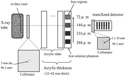
An iron solution phantom is placed between the X-ray tube and the transXend detector. The iron solution phantom comprises 12-mm-thick acrylic and four iron regions of 10 mm thickness. The iron regions are filled with iron nitrate solutions of various concentrations as shown in Figure 1. The effective iron thicknesses of the solutions along the 1 cm of X-ray path length are 72, 144, 216 and 288 μm. The effective iron thickness is estimated by m/ρ, where m is the mass of iron in 1×1×1 cm³ of iron solution and ρ is the density of iron.

Acrylic slabs with thickness of 10 mm are added to increase the acrylic phantom thickness including the iron solution phantom up to 42 mm, since a cylindrical acrylic phantom with diameter of 30 mm is used in the CT measurements in this work. By interpolating the measured current as a function of acrylic thickness, the response functions are estimated in 1-mm intervals of acrylic thickness.

The response function R_i,j is obtained by unfolding the following matrix equation by SANDII code [4].

Here I_n,i is the electric current measured by the ith (i = 1, 6) segment detector when the iron thickness is n μm (n = 0, 72, 144, 216, 288). Y_j,n represents the calculated X-ray events in the energy range E_j when the phantom has iron of n μm thickness. Y_j,n is estimated by calculating X-ray energy spectrum with using the formula of Birch et al. [5], following the X-ray attenuation by the Al filter, air, acrylic and iron, and the integration in the energy range E_j.

2.2. CT measurements

2.2.1. Measurement of a phantom with various concentrations of iron

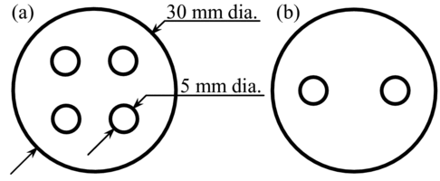
The experimental setup for CT measurements is the same as that shown in Figure 1, but the iron solution phantom and acrylic slabs are replaced by a cylindrical acrylic phantom with the diameter of 30 mm. The cylindrical phantom has four holes with diameter of 5 mm as shown in Figure 2(a) . Each of the four holes is filled with iron nitrate solution having an iron concentration of 50, 100, 150 or 200 μmol/g. For example, an iron concentration of 200 μmol/g corresponds to iron thickness of 144 μm in 5 mm of water. The limit of the iron concentration for healthy liver tissue is 145.4 μmol/g [6].

Figure 2 Schematic drawings of 30-mm-diameter cylindrical phantoms with (a) four holes and (b) two holes. The heights of these phantoms are 60 mm

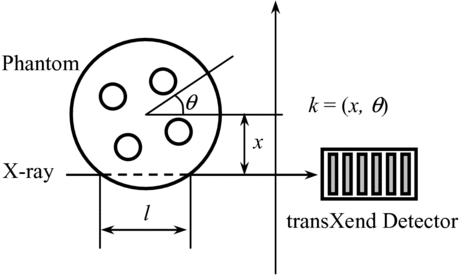
The CT measurements are performed by first-generation CT; i.e. by translating and rotating the phantom. The translation (x) has a step size of 0.4 mm and is repeated 86 times. After the translation, the phantom moves back to its initial position and is rotated through an angle θ of 5°. This measurement is repeated 36 times to rotate the phantom through 180 degrees.

Before starting the unfolding process, the X-ray path length, l, is estimated for each measurement point (x, θ) using the CT image obtained with the current-measurement CT data to choose response functions, which are prepared as functions of the acrylic thickness l. With CT measurement data, the X-ray energy distribution for each measurement point is calculated by unfolding the following matrix using SANDII code.

Here k is the measurement point for given (x, θ). The relationship between x, θ and l to point k is shown in Figure 3 . I_i,k is the electric current value measured by the ith segment detector at measurement point k. Y_j,k denotes the X-ray events in the energy range E_j after passing the phantom at measurement point k.

Figure 3 Relationship between x, θ and l and measurement point k

2.2.2. Measurement of a phantom with iron and adipose

In addition to CT measurements for various concentrations of iron, CT measurements are made for a phantom with iron and adipose (canola oil); liver has adipose as well as soft tissue. The phantom used is shown in Figure 2(b) and has a 5-mm-diameter region of iron solution and a 5-mm-diameter region of adipose. The iron region is filled with iron nitrate solution having an iron concentration of 200 μmol/g. CT measurements are performed in the same way as described in the previous section, but the rotation angle is 10°. The measurement is repeated 18 times to give total rotation of 180°. The X-ray energy distributions are obtained in the same way as described in the previous section.

3. Results and discussion

3.1. Iron of various concentrations

Figure 4 shows CT images of iron solutions of various concentrations obtained by (1) current-measurement CT and (2) energy-resolved CT using the events of X-rays in the energy range E ₁. CT images are reconstructed employing the filtered back-projection method [7].

Figure 4 CT images of iron solutions with concentrations of 50, 100, 150 and 200 μmol/g obtained by (a) current-measurement CT and (b) energy-resolved CT obtained by X-ray events in the energy range E ₁

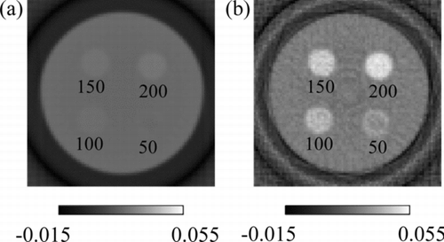
The current-measurement CT image (1) barely shows the 200-μmol/g iron region, whereas the energy-resolved CT image (2) shows iron regions clearly. The energy-resolved CT image looks noisy compared with current-measurement CT image: the image of energy-resolved CT is obtained after calculations using the data of current-measurement CT and cannot avoid deteriorating its quality. On the other hand, the image of current-measurement CT has low contrast to iron, since it uses high energy X-rays with less absorption coefficients. The energy-resolved CT using low energy X-rays, which have high absorption coefficients can tell low concentration iron region.

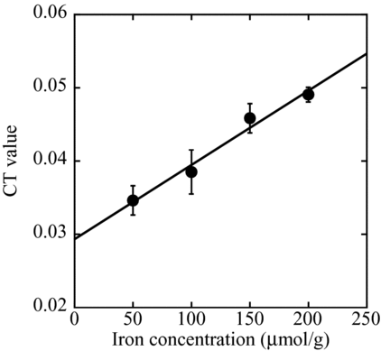
The energy-resolved CT values of iron solutions with concentrations of 50, 100, 150 and 200 μmol/g are 0.035 ± 0.002, 0.038 ± 0.003, 0.045 ± 0.002 and 0.049 ± 0.001, respectively. Here, the CT value of iron is the absorption coefficient of iron solution averaged over the energy range E ₁. The relationship between the iron concentration and the CT value is shown in Figure 5 . The CT value is shown to be proportional to the iron concentration.

Figure 5 Relationship between the iron concentration and CT value

3.2. CT measurement of a phantom with iron and adipose

A CT measurement was performed for the phantom with iron and adipose shown in Figure 2(b). The CT images obtained using the X-ray events in the energy ranges E ₁ and E ₄ are shown in Figure 6(a) and (b) , respectively. The CT value profiles along the centerline of iron and adipose are shown in Figure 7 .

Figure 6 CT images of adipose and iron solution obtained by the X-ray events in the energy ranges (a) E ₁ and (b) E ₄

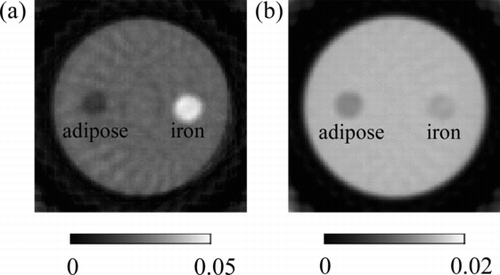
Figure 7 CT value profiles along the centerline of the iron and adipose regions obtained by the X-ray events in the energy ranges E ₁ (solid line) and E ₄ (dashed line), respectively

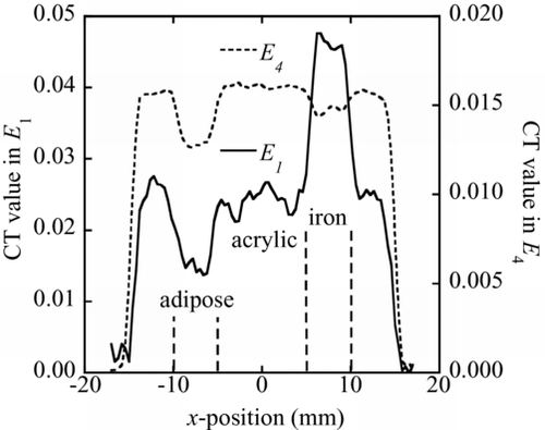
In the energy range E ₁, the CT values of iron and adipose are higher and lower than that of acrylic, respectively. However, the CT values of both iron and adipose are lower than that of acrylic in the energy range E ₄. These behaviors of CT values are explained by the X-ray linear attenuation coefficients. As shown in Figure 8 , linear attenuation coefficients of iron and adipose are higher and lower than that of acrylic in the energy range E ₁. However, linear attenuation coefficients of both iron and adipose are lower than that of acrylic in the energy range E ₄. [8]

Figure 8 Linear attenuation coefficients of iron, adipose and acrylic [8]

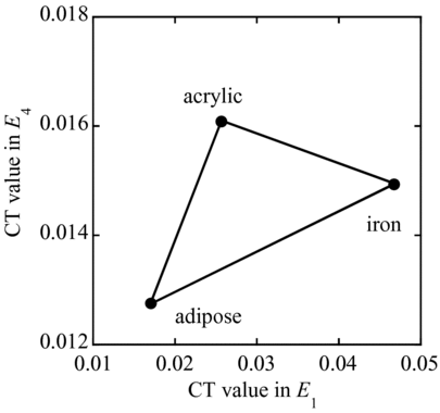
Using the CT values obtained by the X-ray events in E ₁ and E ₄ for iron, adipose and acrylic, a two-dimensional map is drawn as shown in Figure 9 . The point “iron”, for example, indicates the CT values for an iron concentration of 200 μmol/g and no other materials. Likewise, the points “acrylic” and “adipose”, respectively, indicate acrylic and adipose only. When CT values obtained from the X-ray events in the energy ranges E ₁ and E ₄ fall on a point within the triangle, we can determine the portions of acrylic (soft tissue), adipose and iron in the subject under test. For example, when CT values are 0.03 and 0.015 in energy range E ₁ and E ₄, this material is estimated to have 26% of iron, 19% of adipose and 55% of acrylic. Here, 26% of iron is estimated 52 μmol/g: 100% of iron is 200 μmol/g.

Figure 9 Two-dimensional map of CT values obtained by the X-ray events in the energy ranges E ₁ and E ₄ for iron, adipose and acrylic

Two-dimensional map can also be drawn by the dual-energy CT, however, the energy-resolved CT is much informative. For example, when X-ray tube voltages are 80 and 140 kVp, the averaged energies of each X-ray spectrum are about 40 and 55 keV, respectively. The difference of the averaged energy is 15 keV, although the change of tube voltages is 60 kV. On the other hand, the two-dimensional map of the energy-resolved CT can give detailed information with using energy ranges 15–50 and 70–90 keV as shown in Figure 9.

4. Conclusions

Compared with current-measurement CT, energy-resolved CT is superior in detecting iron solution, especially low concentration iron solutions. Using the transXend detector, CT values in more than two energy ranges can be obtained with one measurement. The CT values in different energy ranges can be used to draw a two-dimensional map, which shows the components of the subject. The image of energy-resolved CT is noisy compared with the one of current-measurement CT, however, it is possible to improve the image quality with using smoothing method. As a future study, comparison of the dose exposures in the energy-resolved CT and in the dual-energy CT should be discussed.

Acknowledgements

The authors are grateful to Prof. K. Hitomi of Tohoku University for providing the use of his CT image reconstruction program. Part of this study is supported by a grant-in-aid for Scientific Research from the Japan Society for the Promotion of Science, and the Suzuken Memorial Foundation.

References

- Castiella , A , Alustiza , J M , Emparanza , J I , Zapata , E M , Costero , B and Diez , M I . 2011 . Liver iron concentration quantification by MRI: are recommended protocols accurate enough for clinical practice? . Eur Radiol , 21 : 137 – 141 .
- Shikhaliev , P M . 2008 . Energy-resolved computed tomography: first experimental results . Phys Med Biol , 53 : 5595 – 5613 .
- Kanno , I , Imamura , R , Mikami , K , Uesaka , A , Hashimoto , M , Ohtaka , M , Ara , K , Nomiya , S and Onabe , H . 2008 . A current mode detector for unfolding X-ray energy distribution . J Nucl Sci Technol , 45 : 1165 – 1170 .
- McElroy , W , Berg , S , Crockes , T and Hawkins , G . 1967 . A computer-automated iterative method for neutron flux spectra determination by foil activation , AFWL-TR-67-41, New Mexico: Air Force Weapons Laboratory .
- Birch , B and Marshall , M . 1917 . Computation of Bremsstrahlung X-ray spectra and comparison with spectra measured with a Ge(Li) detector . Phys Med Biol , 24 : 505 – 517 .
- Fischer , M A , Reiner , C S , Raptis , D , Donati , O , Goetti , R , Clavien , P A and Alkadhi , H . 2011 . Quantification of liver iron content with CT—added value of dual-energy . Eur Radiol. , 21 : 1727 – 1732 .
- Shepp , L A and Logan , B F . 1974 . Fourier reconstruction of a head section . IEEE Trans Nucl Sci. , NS21-3 : 21 – 43 .
- Hubbell , J H and Seltzer , S M . 2010 . Tables of X-ray mass attenuation coefficients and mass energy-absorption coefficients from 1 keV to 20 MeV for elements Z = 1 to 92 and 48 additional substances of dosimetric interest , The Physical Measurement Laboratory, The National Institute of Standard and Technology . http://www.nist.gov/pml/data/xraycoef/index.cfm