An optimal model of the representative habit data for complex environmental exposure systems

Abstract

The concept of the representative person recommended by the International Commission on Radiological Protection (ICRP) is difficult to apply to dose assessment to the public because the representative habit data could not be determined in advance for general radiation exposure situations. So, a stylized method for constructing habit data of the representative person is needed to ensure consistency and validity of the dose estimation. This paper presents a generalized model of the representative habit data based on optimization by a linear programming technique to handle complex environmental exposure situations such as radioactive waste disposal. The model is devised in such a way that it can fully embody the ICRP's criteria for the representative person by ensuring the upper 5% exposure in the population and it is applicable to general exposure systems. The model was illustrated for Korea's low- and intermediate-level radioactive waste disposal system to show its applicability to complex exposure systems with multiple scenarios and pathways.

Keywords:

• representative person
• habit data
• linear programming
• exposure pathway
• complex scenario
• dose assessment
• risk assessment
• disposal facility

1. Introduction

We need some reasonable diet or habit data for the exposed people to assess the environmental radiological impact and to determine its compliance with the relevant dose constraint. For this purpose, the International Commission on Radiological Protection (ICRP) has introduced the concept of the ‘average member of the critical group’ or the ‘representative person’ for defining the more highly exposed individual in the population from a particular source or a set of sources of radiation [1,2]. The representative person may be defined such that the probability is less than about 5% that a person drawn at random from the population will receive a greater dose. The radiation protection for the public can be assured when the value of dose to the representative person is less than the dose constraint. In this regard, the ICRP provides guidance for the representative person based on using the 95th percentile in the population data set as the habit data. The method recommended by the ICRP, which is summarized in Table 1 , is devised in such a way that it can represent doses of more highly exposed individuals in the exposure system and ensure the upper 5% exposure in the population.

Table 1 ICRP methods for determining the dose to the representative person [1].

	Calculation method
	Probabilistic	Deterministic
Environmental concentration data	Distribution of the estimated or measured concentration	Single values for parameters
Habit data	Range or fixed values for habit data	Average value for the more highly exposed group or 95th percentile of appropriate national or regional data
Dose coefficient	Fixed value based on age	Fixed value based on age
Dose to the representative person	Method selected by the operator or regulator. The representative person is identified such that the probability is less than about 5% that a person drawn at random from the population will receive a greater dose.	Product of above values

According to the ICRP's guidance [1,2], the representative person should have three important attributes of habit: reasonableness, sustainability and homogeneity. Reasonableness means that the habit data apply realistically to a person within the range of usual life. Sustainability and homogeneity are aspects of reasonableness. Sustainability implies that the selected habits can be continued over the time frame of the assessment. Habit data need to be sustainable. Exposure situations may be considered sustainable when they remain longer than 5 years. Homogeneity deals with the degree to which extremes in particular habit data are, or are not, included in the assessment. It should be carefully avoided to select extreme percentile values for every component of habit to prevent excessive conservatism in the assessment because such a result could lead to unrealistic dose to the representative person and to undue design of radiation sources or facilities. In other words, the parameters of habit data should be selected and combined to represent reasonable and sustainable exposure scenarios. The representative person may be actual or hypothetical, but the habits (e.g., intake rates of foodstuffs) used to characterize the representative person should be typical of the more highly exposed individuals, not a particular extreme one, in the population [2]. In the absence of site-specific data, it may be a reasonable approach to use the 95th percentile of behaviour as an intake rate. In general one exposure pathway for a particular source will dominate the dose to the representative person from that source. If more than one intake route for radionuclides (i.e., exposure pathway) provides a significant contribution to dose, it may not be reasonable to assign the 95th percentile habit data to all routes because it is an extreme case that people cannot encounter in day-to-day life and the total dietary intake is not consistent with the credible personal limit [1,3,4]. In this case, a 95th percentile intake should be allotted to the more dominant pathway, and a lower value should be allotted to other pathways, so as to be consistent with the requirement that the dose assessment be based on a set of habits that are reasonable and sustainable. Even if more than one exposure pathway makes a significant contribution to the summed effective dose, the individuals receiving the highest exposures tend to be fairly homogeneous with regard to habits [3,4].

The ICRP's concept on the representative person summarized above is easily applicable with intuition to simple cases. However, it tends to meet with difficulties in applying to rather practical cases of dose assessment, where several coexisting exposure pathways vary with time, as follows:

1.	The representative person or the habit data, in compliance with the ICRP's guidance, for the dose assessment cannot be determined ahead of the exposure pathways analysis. Since the exposure depends on the radiation level (e.g., concentrations of radionuclides) in the pathways involved, it is needed to calculate doses iteratively with the pathways and radiation levels in order to consider their variations with time.
2.	For risk assessment, the dose and the corresponding risk, which is a function of the probability of an event causing a dose and the probability of detriment due to that dose [2,5], may show different behaviours with each other.
3.	It is another problem to establish a representative person for a complex exposure system with many radiation sources, exposure scenarios and pathways. Since they will evolve independently and/or jointly in such a system, the resultant behaviour may be very complicated in terms of exposure.
4.	To observe the ICRP's concept fully, we should first calculate every individual dose and then sort out the one for the representative person from the population. This is, however, impractical in most cases.

In short, the representative person cannot be predetermined by intuition for general exposure situations and the concept is not easy to apply to the dose assessment. Therefore, we need a stylized method for selecting or constructing the habit data so as to ensure a consistency and validity of dose assessment. This solution should be emphasized for environmental exposure problems such as radioactive waste disposal which show complicated radiological aspects over a long time. In this paper, we develop a technique for establishing the representative person in terms of habit data to apply to general exposure systems and the risk assessment in which exposure situations include multiple scenarios and pathways varying with time.

This paper aims for introducing the newly recommended concept on radiation protection and an implementing method to complex environmental radiological systems. Most of the traditional safety assessments have focused mainly on radionuclide transport and have left something to be desired for its endpoint or environmental dose calculation. This work will improve the endpoint analysis in conjunction with the related recent progress in that field [6,7].

2. Estimation of habit data for the representative person

In an exposure system, a total risk R to an individual can be expressed at a point of time as [8,9]:

where γ denotes the risk coefficient (e.g., 5 × 10⁻² Sv⁻¹) quantifying the probability of harmful health effects of radiation per unit dose [2], E(D) is the expected value of dose D, p(D) is the annual probability of receiving a radiation dose in the range (D, D + dD), p_k is the annual probability of the exposure scenario or pathway k giving rise to annual dose D_k to the individual, c_k is the radiological level of contaminated media or pathway k (e.g., [Bq/kg]), and f_k is the dose coefficient (e.g., [Sv/Bq]) linking the contamination level to dose, w_k is the interaction rate between the receptor and the media (e.g., consumption rate, [kg/yr]) or k-component of the habit data, and N is the number of pathways considered (i.e., 1–N). In this expression, radionuclides are involved in f_k and c_k for simplification, which does not lose its generality through the subsequent development. In expression (1), p_kc_k is the expected value of c_k and w_k is the variable to be determined from habit data of the exposed people. The representative person corresponds, in principle, to the individual with the habit data related to 95th percentile E(D) in the population. Since it is not practical to sort the values by applying every habit data to expression (1), we need a method for narrowing down the range. Noting that E(D) is linear with respect to w, we can consider restricting the level of E(D) by linear combinations of w in the habit data, where each element w has N w-components of the pathway, while excluding extreme data from the ICRP's point of view.

2.1. Approximation by linear programming

Let's consider estimating the data corresponding to xth percentile E(D) in a given exposure system. First, we construct a “representative group” S with xth percentile w's of N pathways and their possible linear combinations from the habit data set in the population P . (We assume P to be fairly large for the calculation purpose so that it has data corresponding or sufficiently close to every percentile.) We express these elements as w ^x _i , w ^x _i,j , … , w ^x _1,2,…,n , where, for example, w ^x _i,j denotes a habit data w including the xth percentile value w^x _i,j in the distribution of w_i + w_j , and then examine whether S may bound a lower x% with respect to E(D) in P .

In order to gain some intuition for that matter, let's consider the following linear programming (LP) problem of a two-component system (w ₁,w ₂) with two pathways:

subject to

In problem (2), the coefficient a of w abbreviates the relevant coefficients to expression (1) (e.g., a_k =f_kp_kc_k ). In addition, in inequality constraints (3)–(5), which restrict the range of pathway combinations, w^x _i denotes the component of pathway i in w ^x _i or the xth percentile value in the distribution of w_i in P , and w^x _i,j represents the sum of components i and j in w ^x _i,j or the xth percentile value in the distribution of w_i + w_j in P .

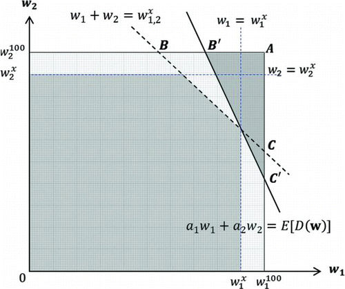
Figure 1 depicts the problem domain, where the LP region is the lower-left-hand shaded pentagon bounded by xth percentile values (i.e., w^x ₁, w^x ₂, w^x _1,2) in the distributions of two pathways (w ₁, w ₂) and their combination (w ₁ + w ₂), and ΔAB′C′ corresponds to the part exceeding the xth percentile with respect to E(D) in the whole P . If ΔAB′C′ is not larger than ΔABC covering (100−x)% in terms of element or data, which is the case for Figure 1, the expected dose E[D(w ^x _LP )] corresponding to data w ^x _LP determined by this LP is not less than E[D(w ^x _P )], the xth percentile expectation in the whole P [10], where w ^x _P is the real data producing 95th percentile E(D) in P . This means that the relation E[D(w ^x _P )]⩽E[D(w ^x _LP )] holds for the convex region w ₁ + w ₂⩽w^x _1,2.

Figure 1 Schematic of a two-variable LP, illustrated with x=90 percentile

Since it can similarly be delineated for systems with more than two components in terms of hyperplanes, the above development can be generalized for systems with N pathways as follows:

for

As it can graphically be seen from Figure 1, such a relation is satisfied with x⩾50 depending on the distributional characteristics of data in P and always holds for x=95.

From the above discussion, we can claim that S constructs a range of data covering the lower 95% with respect to E(D) in the following LP:

subject to

where w is an N-component vector, a is an N-component vector corresponding to the coefficients in expression (1) and the superscript T denotes transpose. Since they are habit data, the values of w ⁰, each of which is the minimum for the corresponding pathway or a combination of pathways, may be replaced by 0. Inequality constraints (11)–(14) should include all the possible independent linear combinations _n C₁, _n C₂, …, _n C _n (total of 2 ⁿ − 1) from N different pathways. Since constraints (11)–(14) cover the lower 95% in P with respect to E(D), the following relation holds between w ⁹⁵ _LP determined from the LP and the 95th percentile E(D) in P , similarly to (6):

where w ⁹⁵ _P denotes the data producing 95th percentile E(D) in P . In inequality (15), the two expectations may approach each other depending on data distributions and their harmony with the coefficient a in problem (10). Therefore, we can practically take w ⁹⁵ _LP , instead of the real w ⁹⁵ _P , as the habit data of the representative person, which may be a reasonably conservative approximation in terms of radiological protection. This may be an optimal choice in a sense that it is based on the linear optimization.

2.2. Sorting out actual habit data

The habit data w ⁹⁵ _LP determined from LP problem (10) is not a real one existing in P but an artificial one compounded to be close to w ⁹⁵ _P . Now we consider sorting out real data close to w ⁹⁵ _P or w ⁹⁵ _LP . The linearity of expression (1) with respect to w indicates that there exists a data close enough to w ⁹⁵ _P and w ⁹⁵ _LP in terms of E(D) in the representative group S. We can find an element w satisfying the following condition, say, w ⁹⁵ _S , which may also be a reasonable substitute for w ⁹⁵ _P :

where a is an N-component vector corresponding to the coefficients in expression (1) and w are N-component vectors. This sorting tries to find a real data yielding a minimal absolute difference of E(D). It may be useful in case the size of S is relevant to the calculation or a manageable number of pathways are involved in the exposure scenarios.

2.3. Selecting habit data for a time interval, scenario or exposure system

In the development above, the habit data w ⁹⁵ _LP or w ⁹⁵ _S determined from problem (10) or (16) is the data corresponding to the radiological level c of pathways involved at that point in time. Since exposure dose should reflect the related exposure situations, w ⁹⁵ _LP or w ⁹⁵ _S is applicable to the dose calculation as a substitute of w ⁹⁵ _P or the habit data of the representative person at a given time point. On the other hand, we may seek for some habit data covering a range of time, an exposure scenario or a system to understand the overall trend. For this purpose, we can select w ⁹⁵ data representing the relevant scope from the distribution of w ⁹⁵ _LP or w ⁹⁵ _S in time. In this case, a heuristic selection may be rather practical in connection with the characteristics of the system or scenarios and the purpose of dose assessment. The potential choices include the habit data which cover a relatively long time span, important peaks (e.g., radionuclide concentration or dose) or time ranges of interest in the assessment.

3. Modelling algorithm and application

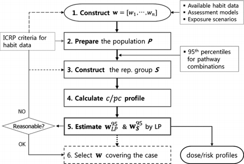
The model developed above may be carried out through the following procedure to determine the representative habit data in the dose/risk assessment for complex exposure systems. Figure 2 outlines the overall procedure.

Figure 2 Procedure to determine the representative habit data

	Step 1. Determine the exposure pathways and how to construct w, taking dose/risk assessment models, exposure scenarios and the available set of habit data into consideration. If the available set of habit data has different pathway items from those which the assessment models and/or inputs allow, arrange the list of pathways properly to the purpose of the assessment.
	Step 2. Prepare the population P by reorganizing the available habit data in accordance with how to construct w. If the assessment is to handle complex scenarios, it is convenient to construct P consistently with the scenario having the most pathways.
	Step 3. Construct S properly to the purpose of the assessment, for each exposure scenario, with 95th percentile w data for the pathway combinations or constraints (11)–(14) while excluding extreme values. For complex scenarios, go through Step 1, 2 and 3 similarly while constructing S to include all the independent pathways (N) involved in individual scenarios.
	Step 4. Carry out the model calculation and obtain c data for each scenario, radionuclide and w component. For risk assessment, prepare a distribution of pc from c profile with occurrence time of the related probabilistic scenario [8,9]. In this model, radionuclides are involved in fk , ck and ak for the convenience of development. So, a real application should yield these values for each radionuclide and integrate them.
	Step 5. Perform problems (10) and (16) at relevant time intervals for the scenarios using c or pc profiles with time. Once ak in problem (10) are prepared, the subsequent LP calculation is straightforward, which can be carried out with one of many available computer programs for LP. Check w 95 LP first and determine whether there is a need to sort out w 95 S from S or not. Examine w 95 LP and w 95 S whether they are in accordance with the purpose of the assessment and the ICRP's concept.
	Step 6. If necessary, select or determine a w data covering the exposure scenario or whole system based on the distributions of w 95 LP and w 95 S over time.

3.1. Considering different kinds of exposure scenarios

It is desirable to group food pathways into a category in that there is a limit for a person to intake them. On the other side, some pathways related to the breathing rate or parameters contributing to external exposure (e.g., residence time) are much independent of food pathways. In addition, drinking water pathways may also show a different tendency from ordinary food pathways. Since it guarantees E(D) not less than 95th percentile, the model developed above is, in principle, applicable to any pathways regardless of their individual characteristics. It can handle different kinds of pathways in a lump even with different units. However, considering that the size of data and constraints to be dealt with increases with the number of pathways, it may be also reasonable to assign 95th percentile w values for the peculiar pathways. Since it will result in higher E(D), the corresponding representative habit data may be a conservative one for the pathways in the system.

3.2. Application to complex exposure systems

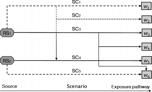
An exposure system can include two or more radiation sources, exposure scenarios and pathways. For example, two different disposal facilities may be developed in a site over a period of time. Figure 3 shows such a complex system comprising five scenarios and six pathways derived from two sources. (In the figure, the dotted lines indicate potential pathways associated with probabilistic scenarios.) The exposure occurs through the related pathways whatever contents the system has and however the sources and scenarios are involved in each other. In other words, we have only to sum up the relevant pathways under the given situation in terms of exposure [8]. Since expression (1) is expressed for such an integrated analysis, the method developed above to establish the representative habit data is generalized in itself for complex systems.

As an example, consider two different (i.e., independent) scenarios A and B which have four and three pathways, respectively. First, in order to determine the representative habit data for scenario A , we should sort out 95th percentile w data (total of 2⁴ − 1) for all the possible independent linear combinations from four basic pathways (=₄C₁ + ₄C₂ + ₄C₃ + ₄C₄) and construct the representative group S _A with them to solve problems (10) and (16). For B , the same as the procedure for A , we can determine the representative habit data from problems (10) and (16) based on the representative group S _B with 2³ − 1 95th percentile w data for ₃C₁ + ₃C₂ + ₃C₃ linear combinations from three basic pathways.

Now we consider a case with scenarios A and B at a time. Assuming one pathway overlaps in the two scenarios, the composite or complex scenario comprises six independent pathways (=4+3−1). In this case, the same as the case of a single scenario, we have only to sort out 95th percentile w data (total of 2⁶ − 1=63) for all the possible independent linear combinations from six basic pathways (=₆C₁ + ₆C₂ + ₆C₃ + ₆C₄ + ₆C₅ + ₆C₆), construct the whole representative group S _{A + B} with them, and solve problems (10) and (16) again to determine the representative habit data for the complex scenario. In this expansion, the total of 63 w data consists of 21 (=15+7−1) from S _A and S _B and 42 from interactions between S _A and S _B .

In this manner, the number of w data organizing the representative group tends to increase exponentially with the number of pathways in order that the LP domain may be constructed as close as to the related structure of P with a indicating exposure characteristics in problem (10). Many complex scenarios will include probabilistic ones. For these cases, there is a need to widen the range of assessment in harmony with the potential exposure situations. This model basically involves such a consideration.

3.3. Consideration for risk assessment

Expression (1), which is the base of the model development, is generalized in itself with respect to risk assessment. However, it is additionally needed for risk assessment to express the radiological level (c_k ) of the pathway as its expectation (p_kc_k ) combined with the probability, as in expression (1). This is because the representative habit data should be based on the expected value of c_k as it is not simply dose D but expected dose E(D) to be associated with the representative person in terms of risk at a point in time. Since the time when a scenario begins is not the same in general as the time of the subsequent exposure, it is needed to obtain the profile of p_kc_k with time in advance of determining the representative habit data and the expected dose or risk.

4. Illustration

We demonstrate the model described above through a real case of dose assessment. The problem is for the environmental exposure calculation in the post-closure safety assessment of the Wolsong low- and intermediate-level radioactive waste disposal facility in Korea [11], which is briefly introduced in Table 2 .

According to the regulation [12], the assessment requires dealing with the following three categories of scenarios:

A.	Normal scenario . This category includes natural likely processes through which radionuclides migrate from repository to biosphere to give a dose (e.g., gradual transport of radionuclides with groundwater). The dose constraint is 0.1 mSv/yr for this scenario.
B.	Abnormal scenario . This covers natural probabilistic events (e.g., disruption of engineered barriers by earthquake) which may cause, for example, rapid release of radionuclides from repository. The risk constraint is 10−6 /yr for this scenario.
C.	Intrusion scenario . This means accidental access of human to repository which may result in an increase of radiation exposure (e.g., drilling a well in the disposal site). The individual dose should not exceed 1 mSv/yr for any reasonable intrusion scenario. In addition, as an example for risk assessment, this illustration considers a complex scenario involving the three in a lump as follows:
D.	Complex case . This integrates the situations where scenarios A, B and C occur with their individual probabilities to contribute to expected dose or risk.

In case that there is no available site-specific habit data for environmental dose assessment, appropriate national or regional information may be used instead [1]. In this illustration, we use a nationwide survey data in Korea [13,14]. In addition, for simplicity we consider only the adult age category, which may be reasonable considering the long-term prospective assessment for repository. Table 3 arranges the habit data of 6705 Korean adults, which is the population P , in terms of food pathways related to this illustration. We can rearrange them for the scenarios.

Table 2 Disposal system information used in the illust-ration [9].

Specification	Description
Name	Wolsong LILW Disposal Center
Location	East coastal area of Gyeongju, Korea
Disposal capacity	100,000 low- and intermediate-level radioactive waste packages (35,200 m^3)
Disposal units	Six underground concrete silos (EL. −130 to −80 m)
Host rock	Fresh granite formation
Groundwater level	EL. 100 m (West Hillock) to EL. 0 m (East Coast)

Table 3 A summary of habit data: food consumption rate of Korean adults.

Consumption rate of food per person [kg/yr]
	6705 persons aged over 17 years
Food group	Maximum	95th percentile	Mean	Median	5th percentile	Minimum
Drinking water	1825.0	730.0	364.3	365.0	146.0	0.0
Grains	528.4	169.4	94.1	90.0	27.8	0.0
Processed grain products	502.9	102.9	23.8	0.0	0.0	0.0
Legumes	357.7	50.0	12.4	4.8	0.0	0.0
Vegetables, kimchi	541.9	136.2	53.3	40.8	1.1	0.0
Vegetables, leafy	518.3	146.5	53.1	40.9	1.1	0.0
Vegetables, root	503.8	89.7	28.2	18.2	0.1	0.0
Fruit vegetables	745.3	85.1	14.1	0.0	0.0	0.0
Fruit	910.6	108.0	17.9	0.6	0.0	0.0
Fish	391.4	73.0	16.0	2.7	0.0	0.0
Shellfish	276.3	20.9	3.8	0.0	0.0	0.0
Mollusks	228.1	20.1	3.2	0.0	0.0	0.0
Marine plants	182.8	21.9	3.8	0.2	0.0	0.0

Due to the long time-scales in the safety assessment of the repository, the future human habits can only be assumed. Consequently, in order to avoid unnecessary speculation and uncertainty, the future generations’ habits should be chosen on the basis of some reasonably conservative, stylized approaches, considering current lifestyles and the available specific or more general conditions [15,16]. In this context, the present statistical data for human habits can also be applied to the assessment for future exposure by means of the representative person.

A. Estimation for the normal scenario

The repository adjoins the coast and the contaminated groundwater flows directly into the sea. The site-specific analysis shows that the normal exposure will occur mainly in the ocean biosphere because the likelihood of well water and land use will also be very low in the future as is present [11]. We consider the following three pathways by way of groundwater to assess the doses to future residents neighbouring on the repository.

•	Pathway 1. Fish (k=1);
•	Pathway 2. Shellfish + mollusks (k=2);
•	Pathway 3. Marine plants (k=3).

We sort out the 95th percentile data ( S _A ), like Table 4 , from the population P for seven independent linear combinations from three pathway components to apply to the model calculation for the normal scenario.

Table 4 The representative group for the normal scenario.

Consumption rate of food [kg/yr]
S A	Fish	Shellfish + mollusks	Marine plants	Pathway combination
	(1)	(2)	(3)	(1+2)	(1+3)	(2+3)	(1+2+3)
Data	w 1	w 2	w 3	w 1,2	w 1,3	w 2,3	w 1,2,3
w 1	72.98	31.52	0.00	104.50	72.98	31.52	104.50
w 2	8.94	36.24	0.44	45.18	9.37	36.68	45.61
w 3	27.97	2.22	21.87	30.19	49.84	24.09	52.06
w 1,2	77.16	16.68	0.88	93.84	78.04	17.55	94.72
w 1,3	65.48	15.70	17.37	81.18	82.85	33.06	98.55
w 2,3	4.92	2.93	48.57	7.86	53.50	51.51	56.43
w 1,2,3	1.20	100.53	0.73	101.73	1.93	101.26	102.46

In Table 4, each habit data w in the data column indicates an individual corresponding to 95th percentile in P in terms of the diagonal component of the pathway or pathway combination. For example, w ₃ is equivalent to the person whose annual consumption rate for pathway 3 (i.e., 21.87 kg/yr) corresponds to 95th percentile in the distribution on the component in P .

In this assessment, the important radionuclides to make a contribution to dose are H-3, C-14, Ni-59 and I-129, which account for most of the inventory and show major peaks through thousands of years. The low-level radioactive waste to be disposed of in the repository includes little amount of alpha emitters. The short-lived beta emitter H-3 (half-life = 12.3 yr) appears most rapidly in the environment due to its low affinity to solid phase. The long-lived beta emitter C-14 (half-life = 5.73×10³ yr) shows the highest peak with relatively high affinity to solid phase. Ni-59 (half-life = 7.60×10⁴ yr) appears late due to its long half-life and high affinity. In addition, I-129 (half-life = 1.57×10⁷ yr) is important in that it is a low-affinitive but very long lived radionuclide. We perform model calculations on the radionuclide transport to obtain their concentration profiles for the three pathways, as shown in Figure 4 .

Figure 3 A complex system with two sources, five scenarios and six pathways

Figure 4 Radionuclide concentration profiles for the normal scenario

We need to first determine the coefficient a_k to solve the LP problem (10). For this purpose, we calculate a_k at important points of time using the dose coefficient f for each radionuclide.

Now we solve the LP problem (10). Determine w(w ₁, w ₂, w ₃) maximizing F(w)=a ₁ w ₁ + a ₂ w ₂ + a ₃ w ₃ by LP with the following constraints from Table 4 on S _A :

Solve, if necessary, problem (16) using the LP result w ⁹⁵ _LP to find w ⁹⁵ _S in S _A . As the representative person's habit data, the resulting values of w ⁹⁵ _LP and w ⁹⁵ _S are applicable to the dose assessment for the exposure situation expected “at that time point” after the closure of the repository.

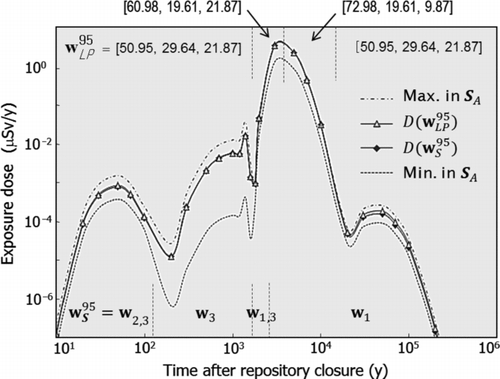
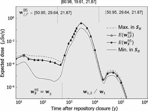
By repeating the above process for relevant points in time, we can obtain the distribution of representative habit data and the corresponding profiles of dose as shown in Figure 5 .

Figure 5 Distributions of the habit data and the exposure dose for the normal scenario

As shown in the figure, there is a little difference between w ⁹⁵ _LP and w ⁹⁵ _S over the time frame and each representative habit data holds for quite a long time. Since it produces much lower dose through the important early (e.g., 1000) years than the other ones in S _A while covering the longest period of time, w ₁ is not appropriate as the overall representative habit data for the safety assessment. On the other hand, w ⁹⁵ _LP 's show similar values with each other in terms of both habit data and dose. Therefore, we can select [w ₁ = 50.95; w ₂ = 29.64; w ₃ = 21.87] as an overall representative habit data for the scenario, which covers a relatively long time, including a range of interest in the assessment.

Figure 5 also includes the maximum and minimum dose profiles obtainable from S _A . As shown in the figure, the maximum profile is similar to those corresponding to w ⁹⁵ _LP and w ⁹⁵ _S , while the minimum is much lower in some period. This implies that there may be big deviations in terms of dose even among 95th percentile data, which indicates the significance of the model developed.

B. Estimation for the abnormal scenario

Assume a probabilistic event that an earthquake disrupts the engineered barriers and increases radionuclide release from the disposal unit, while the radionuclide transport pathways are similar to those in scenario A [11]. Once again, we consider three marine pathways the same as for case A.

•	Pathway 1. Fish (k=1);
•	Pathway 2. Shellfish + mollusks (k=2);
•	Pathway 3. Marine plants (k=3).

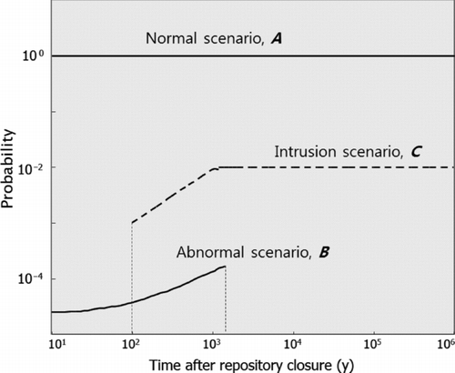
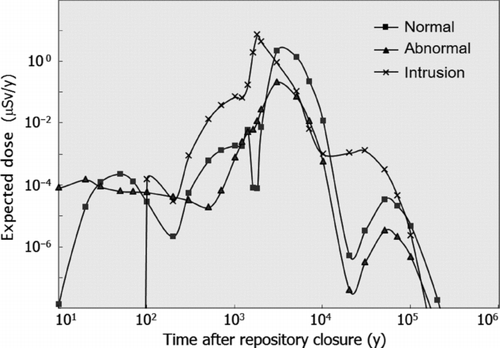
Since the pathways are the same for the two cases, the 95th percentile data ( S _B ) is also the same as S _A . In addition, the important radionuclides are also the same for the two scenarios as H-3, C-14, Ni-59 and I-129. We perform model calculations on the radionuclide transport and apply a probability distribution (given in Figure 10) for the scenario to obtain their expected concentration (pc) profiles for the three pathways, as shown in Figure 6 .

Figure 6 Expected concentration (pc) profiles for the abnormal scenario

Figure 7 Distributions of the habit data and the expected dose for the abnormal scenario

Figure 8 Radionuclide concentration profiles for the intrusion scenario

Figure 9 Distributions of the habit data and the exposure dose for the intrusion scenario

Figure 10 Probability distributions with time for the three scenarios

Following the same subsequent process as for scenario A, we can obtain the distribution of representative habit data and the corresponding profiles of expected dose, as shown in Figure 7 .

As shown in the figure, similarly to case A, there is a little difference in terms of E(D) between w ⁹⁵ _LP and w ⁹⁵ _S over the time frame and each representative habit data holds for quite a long time. As for w ⁹⁵ _LP , [60.98, 19.61, 21.87] or simply [60, 20, 22] can be selected as an overall representative habit data for the scenario. In addition, as a real representative habit data, w _1,3 or [65.48, 15.70, 17.37] may be used for the scenario. We can also recognize from the figure that the maximum profile obtainable from S _A is similar to those corresponding to w ⁹⁵ _LP and w ⁹⁵ _S , while the minimum profile is much lower in some period.

C. Estimation for the intrusion scenario

Assume an intrusion scenario with three different pathways related to using a well on the repository site.

•	Pathway 4. Drinking water (k=4);
•	Pathway 5. Grains + fruits (k=5);
•	Pathway 6. Vegetables (k=6).

The procedure to obtain the representative habit data is the same as for case A. We sort out the 95th percentile data (S_C ), like that given in Table 5 , from the population P for seven independent linear combinations from three pathway components to apply to the model calculation for the intrusion scenario.

Table 5 The representative group for the intrusion scenario.

Consumption rate of food [kg/yr]
SC	Drinking water	Grains + fruits	Vegetables	Pathway combination
	(4)	(5)	(6)	(4+5)	(4+6)	(5+6)	(4+5+6)
Data	w 4	w 5	w 6	w 4,5	w 4,6	w 5,6	w 4,5,6
w 4	730.00	119.80	253.49	849.80	983.49	373.29	1103.29
w 5	219.00	336.54	58.05	555.54	277.05	394.59	613.59
w 6	438.00	198.05	286.27	636.05	724.27	484.31	922.31
w 4,5	584.00	339.96	144.95	923.96	728.95	484.92	1068.92
w 4,6	730.00	174.92	167.97	904.92	897.97	342.88	1072.88
w 5,6	219.00	339.48	217.63	558.48	436.63	557.11	776.11
w 4,5,6	730.00	167.01	228.75	897.01	958.75	395.75	1125.75

As in Table 4, each habit data w in the data column indicates an individual corresponding to 95th percentile in P in terms of the diagonal component of the pathway or pathway combination. The important radionuclides are also the same for this scenario as H-3, C-14, Ni-59 and I-129. We perform model calculations on the radionuclide transport to obtain their concentration profiles for the pathways 4, 5 and 6 as shown in Figure 8 .

Now we solve the LP problem (10). Determine w(w ₄, w ₅, w ₆) maximizing F(w)=a ₄ w ₄ + a ₅ w ₅ + a ₆ w ₆ by LP with the following constraints from Table 5 on S_C :

Solve, if necessary, problem (16) using the LP result w ⁹⁵ _LP to find w ⁹⁵ _S in S_C . As the representative person's habit data, the resulting values of w ⁹⁵ _LP and w ⁹⁵ _S are applicable to the dose assessment for the exposure situation expected “at that time point” after the closure of the repository.

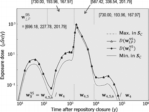
By repeating the above process for relevant points in time, we can obtain the distribution of representative habit data and the corresponding profiles of dose, as shown in Figure 9 .

As shown in the figure, there is a little difference between w ⁹⁵ _LP and w ⁹⁵ _S over the time frame and each representative habit data holds for quite a long time. While both w _4,5,6 and w ₄ cover a longer period of time, w _4,5,6 [w ₄=730.00; w ₅=167.01; w ₆=228.75] is relatively closer to w ⁹⁵ _LP through the time frame. So, w _4,5,6 is applicable as a real representative habit data over the scenario. As for w ⁹⁵ _LP , the four data in the figure show a similar tendency. So, we can use any one of the four or simply [w ₄=700; w ₅=220; w ₆=200] as an overall representative habit data for the scenario.

D. Estimation for the complex case

Finally, we consider a problem with total dose expectation or risk assessment in which the previous scenarios A, B and C all appear together. This complex case involves six different pathways. We should sort out the 95th percentile data from the population P for 63 independent linear combinations from six pathway components to construct the representative group S _{A + C} for this case, 14 elements of which are the same as those from S _A and S_C . We apply probability distributions given in Figure 10 for the three subordinate scenarios to estimate a total expected dose or risk. The engineered barriers are assumed to be degraded completely in about 1400 years, after which the abnormal scenario does not work any longer [11].

As for scenario B, the previous expected concentration (pc) profiles can be reused to obtain expected radionuclide concentrations by pathways. The expected concentration profiles for scenarios A and C can also be produced in a similar way. Now we can solve the LP problem (10) with 63 pathway combinations or constraints (11)–(14). Once a set of the constraints is set up on the LP program, the subsequent calculations can easily proceed with the LP coefficients (i.e., a ₁–a ₆) related to concentrations changing in time.

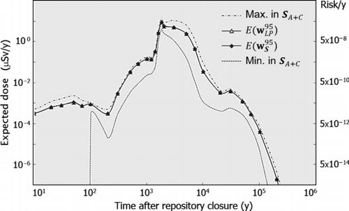
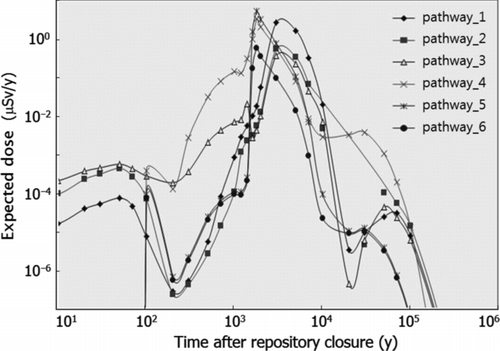
Based on a resulting distribution of representative habit data in time, Figure 11 shows the total expected dose profiles and the total risk due to one normal exposure scenario and two potential exposure scenarios. Since they vary repeatedly with time, w ⁹⁵ _LP and w ⁹⁵ _S are not put in the figure. Such variation indicates that the exposure and risk situations are changeable as the scenarios and pathways increase. In spite of the variation, we can carry out an overall analysis to sort out w _2,6 [234.35, 54.75, 0.00, 365.00, 142.97, 248.66] and/or w _1,2,4,5,6 [48.90, 54.56, 0.22, 584.00, 152.89, 320.04] as the representative habit data throughout the assessment.

Figure 11 Expected dose and risk profiles for the complex case

Figure 12 shows the expected w ⁹⁵ _LP dose contributions by the three individual scenarios to the total dose expectation. In addition, Figure 13 shows the expected w ⁹⁵ _LP dose contributions by the pathways to the total dose expectation.

Figure 12 Expected w ⁹⁵ _LP dose contributions by the three scenarios in the complex case

Figure 13 Expected w ⁹⁵ _LP dose contributions by the pathways in the complex scenario

5. Concluding remarks

The concept of the representative person recommended by the ICRP can be applied to the environmental dose assessment to ensure radiological protection for the public. However, since the representative person cannot be predetermined in general exposure systems, we need a stylized method to construct the representative habit data in accordance with the concept and the purpose of the assessment. In this paper, we developed a generalized model of the representative person, based on the LP, to sort out the habit data consistent with such premises. The model is widely applicable to general or complex systems of dose and risk assessment while well embodying the concept of the representative person. For example, in an independent assessment or evaluation, it can be used to examine the validity of exposure dose calculation and its level of conservatism. Some environmental assessments involving complicated processes on the radionuclide transport often tend to show relatively obscure biosphere modelling and dose calculation. The model also enables us to clearly understand the exposure pathways and their possible interactions.

Nomenclature

a	=	Coefficient vector in the LP problem
a	=	Coefficient or constant in the LP problem (ak =fkpkck )
c	=	Radiological level of the contaminated media or pathway
D	=	Dose
E(D)	=	Expected value of dose D
f	=	Dose coefficient (e.g., [Sv/Bq]) linking the contamination level to dose
N	=	Number of pathways considered or independent components of the habit data
p(D)	=	Annual probability of receiving a radiation dose in the range (D, D + dD)
pk	=	Probability of the exposure scenario or pathwayk giving rise to dose Dk
P	=	Population
R	=	Risk
S	=	Representative group in the population
w	=	Habit data, N-dimensional column vector
w	=	Component of the habit data or interaction rate between the receptor and medium
Greek Letter	=	γ Risk coefficient or probability of harmful health effects of radiation per unit dose
Subscripts	=	1–N Components of habit data or exposure pathways
A–D	=	Exposure scenarios
i, j, k	=	Components of habit data or exposure pathways
LP	=	Component value determined by LP
P	=	Component value existing in the population P
S	=	Component value existing in the representative group S
Superscripts	=	0, 95 Percentile values
T	=	Transpose of a vector
x	=	xth percentile value

Acknowledgements

This work was carried out under the JSPS RONPAKU (PhD dissertation) Program of the Japan Society for the Promotion of Science, partly supported by the National Research Foundation of Korea.

References

- 2006 . Assessing dose of the representative person for the purpose of radiation protection of the public and the optimization of radiological protection: broadening the process , International Commission on Radiological Protection . ICRP Publication 101
- 2007 . The 2007 recommendations of the International Commission on Radiological Protection , International Commission on Radiological Protection, ICRP Publication 103 .
- Hunt , G J , Hewett , C J and Shepard , J G . 1982 . The identification of critical groups and its application to fish and shellfish consumers in the coastal area of the Northeast Irish Sea . Health Phys. , 43 : 875 – 889 . doi: 10.1097/00004032-198212000-00009
- Hunt , G J . 2004 . On homogeneity within the critical group . J Radiol Prot. , 24 : 265 – 272 . doi: 10.1088/0952-4746/24/3/005
- 1996 . International basic safety standards for protection against ionizing radiation and for the safety of radiation sources , Vienna : International Atomic Energy Agency . (Safety Series No. 115)
- Wakasugi , K , Ishiguro , K , Ebashi , T , Ueda , H , Koyama , T , Shiratsuchi , H , Yashio , S and Kawamura , H . 2012 . A methodology for scenario development based on understanding of long-term evolution of geological disposal systems . J Nucl Sci Tech , 49 ( 7 ) : 673 – 688 . doi: 10.1080/00223131.2012.693884
- Hirano , M , Yonomoto , T , Ishigaki , M , Watanabe , N , Maruyama , Y , Sibamoto , Y , Watanabe , T and Moriyama , K . 2012 . Insights from review and analysis of the Fukushima Dai-ichi accident . J Nucl Sci Tech , 49 ( 1 ) : 1 – 17 . doi: 10.1080/18811248.2011.636538
- Seo , E J , Jeong , C W and Sato , S . 2010 . An integrated approach to risk-based post-closure safety evaluation of complex radiation exposure situations in radioactive waste disposal . J Radiat Prot , 35 ( 1) : 6 – 11 .
- Seo , E J , Jeong , C W and Sato , S . 2012 . Application of risk-based approach to post-closure safety assessment in radioactive waste disposal: an integration of complex radiation exposure situations . Ann Nucl Energy. , 49 : 96 – 101 . doi: 10.1016/j.anucene.2012.06.016
- Luenberger , D G . 1984 . Linear and nonlinear programming , 2nd ed. (Chapter 2, ISBN 0-201-15794-2)
- Park , J B , Jung , H , Lee , E Y , Kim , C L , Kim , G Y , Kim , K S , Koh , Y K , Park , K W , Cheong , J H , Jeong , C W , Choi , J S and Kim , K D . 2009 . Wolsong low- and intermediate-level radioactive waste disposal center: progress and challenges . Nucl Eng Tech. , 41 ( 4) : 477 – 492 . doi: 10.5516/NET.2009.41.4.477
- 2012 . Radiological protection criteria for long-term safety on LILW disposal , Seoul : Korea Nuclear Safety and Security Commission .
- 2006 . 2005 Korea National Health and Nutrition Examination Survey , Seoul : Korean Ministry of Health and Welfare . [in Korean]
- 2009 . Improvement of environmental radiation monitoring and radiological assessment methodologies: part B. off-site dose calculation , Seoul : Korea Hydro & Nuclear Power Co. Ltd. . [in Korean]
- 2000 . Radiation protection recommendations as applied to the disposal of long-lived radioactive waste , Ontario : International Commission on Radiological Protection .
- 2003 . “Reference Biospheres” for solid radioactive waste disposal. Report of BIOMASS Theme 1 of the BIOsphere Modelling and ASSessment (BIOMASS) Programme , Vienna : International Atomic Energy Agency .