Prediction of temperature and water level in a spent fuel pit during loss of all AC power supplies

^†This is a translation of an article originally published in Japanese in Transactions of the Atomic Energy Society of Japan <http://dx.doi.org/10.3327/taesj.J11.050>. Taylor & Francis do not warrant the accuracy of the translation.

Abstract

A prediction method for water temperature in a spent fuel pit of a pressurized water reactor (PWR) has been developed to calculate the increase in water temperature during the shutdown of cooling systems. In this study, the prediction method was extended to calculate the water level in a spent fuel pit during loss of all AC power supplies, and predicted results were compared with measured values of spent fuel pools in the Fukushima Daiichi Nuclear Power Station. The calculations gave reasonable results, but overestimated the decreasing rate of the water level and the water temperature. This indicated that decay heat was overestimated and evaporation heat transfer from the water surface was underestimated. Results of calculations with 80% decay heat and 155% (Unit 4 pool) or 230% (Unit 2 pool) evaporation heat flux were in good agreement with measured values. The data-fitted evaporation heat fluxes agreed rather well with the evaporation heat transfer correlation proposed by Fujii et al.

Keywords:

• spent fuel pit
• loss of all AC power supplies
• decay heat
• evaporation
• water temperature
• water level
• the Fukushima Daiichi Nuclear Power Station

1. Introduction

A spent fuel pit (or spent fuel pool, hereafter SFP) in a nuclear power plant is generally equipped with two cooling systems to remove decay heat from spent fuel assemblies and to keep the SFP water at a low temperature. Above the water surface of the SFP, an air curtain is formed by air ventilation systems, which are normally operated by external AC power supplies or by emergency diesel generators when external AC power supplies fail. Evaluating the increase in the SFP water temperature and the time until the upper limit of the SFP water temperature is reached becomes important during the shutdown of cooling systems. On the other hand, evaluating the water level in the SFP becomes important during loss of all AC power supplies including the emergency diesel generators. Important uncertainties for prediction of the water temperature and water level in the SFP during the shutdown of cooling systems and air ventilation systems are decay heat and evaporation heat transfer from the water surface to air in the fuel handling building.

The normal water level in the SFP is about 7 m above the top of the spent fuel racks and this is a large amount of water to provide gamma radiation shielding. Therefore, the water temperature increasing rate and water level decreasing rate in the SFP are very small, and these issues have been rarely reported. For decommissioning of a nuclear power plant, the USNRC has reported the time limit and the cooling period needed to ensure no damage to spent fuel assemblies when they are exposed in the air during loss of all AC power supplies [1]. However, the report calculations focused on the cooling period and an adiabatic condition was used. The adiabatic condition means that heat losses from the SFP water to air and concrete are neglected. The adiabatic condition also means that all decay heat is stored in the water before reaching 100 °C or all decay heat is consumed in boiling after reaching 100 °C. There is a big difference in prediction of the water temperature between heat loss and the adiabatic condition in some cases.

In serial studies [2–4], a correlation for evaporation of heat fluxes from water surface to air during the shutdown of cooling systems was derived [2], and based on the three-dimensional (3D) thermal hydraulic behavior calculated by using CFD software [3], the water temperature prediction system with a one-region model was developed [4]. In this paper, this prediction system has been extended to calculate the water level in the SFP during loss of all AC power supplies, and predicted results have been verified using measured values in SFPs of the Fukushima Daiichi Nuclear Power Station [5].

2. Outline of the water temperature prediction system during shutdown of cooling systems

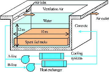
Figure 1 shows a conceptual diagram of a pressurized water reactor (PWR) SFP. The SFP layout differs among reactor types. Further, the SFP is generally located in the fuel handling building outside of the reactor building in a PWR and on the operation floor in the reactor building in a BWR (boiling water reactor) [6]. The inside wall of the SFP is covered with stainless steel. The water depth of the SFP is about 12 m. The width and length of the SFP below the water surface are also different, depending on the plant capacity, but these are about 10 m × 10 m.

Figure 1. Conceptual diagram of a PWR spent fuel pit.

Prediction of water level during the loss of all AC power supplies in this study was added to the water temperature prediction system [4] during the shutdown of cooling systems. The water temperature prediction system consists of a database for spent fuel assemblies, a subsystem to calculate decay heat of spent fuel assemblies, and a subsystem to calculate the water temperature and level in the SFP.

2.1. Prediction of decay heat

The burn-up calculation software, ORIGEN 2.2 [7], and the nuclear cross-section libraries [8] for ORIGEN 2 based on JENDL 3.3 [9] were used to calculate decay heat of fuel assemblies. Calculation conditions were for uranium fuel assemblies of PWRs and the maximum burn-up was 48 GWd/t or 55 GWd/t with three cycles. Decay heat of the shutdown reactor core was calculated for operation periods of 3, 6, and 13 months and the operation period to reach the maximum burn-up with an equivalent mixture of three-cycle burn-up fuel assemblies, and the tables of decay heat were made with the parameters of these four operation periods and the cooling time after the reactor shutdown. Decay heat of spent fuel assemblies stored in the SFP was treated for the maximum burn-up fuel assemblies and calculated after the reactor shutdown, and the tables of decay heat were made for the time after the reactor shutdown. From the data of the spent fuel assemblies stored in the SFP, respective decay heat of each fuel assembly was calculated using the tables of decay heat.

2.2. Prediction of water temperature and water level

The previous study [3] showed the water temperature in the rack was higher than the average water temperature due to the decay heat and was almost uniform outside the rack, except for regions near the water surface and the concrete walls. Therefore, in the developed predicting water temperature system [4], the average water temperature was calculated with the one-region model of the SFP water, and the water surface temperature, which was used for calculating evaporation heat fluxes from the water surface to air, was calculated separately. The heat balance equation for the one-region model consisted of decay heat as heat source, heat stored in water, heat transfer from water to concrete, and evaporation heat transfer from the water surface to air. Heat transfer from water to concrete and heat distribution in concrete were calculated using the 1D unsteady heat conduction equation with the natural convection heat transfer correlation proposed by Kataoka et al. [10]. Thermal resistance of the stainless steel covering on the SFP wall was small, so it was neglected. Evaporation heat transfer from the water surface to air was calculated using water surface temperature and the correlation proposed by Yanagi et al. [2] for evaporation heat flux. Calculation of water surface temperature requires the natural circulation flow rate near the water surface. This natural circulation flow rate was obtained and good agreement was seen between water temperatures (both average water temperature and water surface temperature) computed by the 3D simulation and one-region model. Then a correlation for natural circulation flow rates was derived as a function of decay heat and this was introduced into the water temperature prediction system with the one-region model.

The water temperature is limited to values lower than 65 °C by technical specifications under normal operating conditions. For normal operating conditions, the water level is almost constant but this prediction system was extended to predict water level during loss of all AC power supplies. The heat balance equation for the one-region model introduced evaporation from the water surface to air before the water temperature reached the saturated temperature (100 °C), and introduced boiling after the water temperature reached the saturated temperature. (The difference between decay heat and heat transfer from water to concrete equals the total of evaporation heat transfer and boiling heat.) Radiation heat transfer does not affect the decease of water mass. Because of the uncertain emissivity and the small effect on the calculation of water mass even with the emissivity of 1.0, radiation heat transfer was not considered in this prediction system. Fluid properties were obtained as functions of temperature and the water level was calculated from the water mass, the water density, the water surface area, and the water expansion.

2.3. Correlation for evaporation heat fluxes

The correlation used for evaporation heat fluxes from the water surface to air q_E (kW/m²) was given by the following equation proposed by Yanagi et al. [2] for forced convection air flow: (1) $$\begin{array}{c}\hfill q_E=0.010{\rho }_a{U}_a^{0.60}\left(\frac{0.622P_{S0}}{P-0.378P_{S0}}-\frac{0.622P_{\mathrm{S}\infty }}{P-0.378P_{S\infty }}\right)h_{fg},\end{array}$$(1) where h_fg (kJ/kg) is the latent heat of evaporation, P (Pa) is the system pressure, P_S0 (Pa) is the saturated vapor pressure on the water surface, P_S∞ (Pa) is the vapor pressure in air, U_a (m/s) is the air velocity, and ρ_a (kg/m³) is the air density. The first and second fractions in Equation (1) are vapor weight ratios on the water surface and in bulk air, respectively. Equation (1) contains both convection and radiation heat transfers in the measured water temperature range of 20–65 °C.

The correlation used for evaporation heat fluxes from the water surface to air inside the fuel handling building q_E (kW/m²) was Equation (2) [2]. The equation for natural convection air flow was derived from the analogy between natural convection heat transfer and mass transfer of vapor to evaluate the coexisting field with forced convection and natural convection: (2) $$\begin{array}{ccc}\hfill q_E& =& h_D{\rho }_{\mathrm{a}}\left(\frac{0.622P_{S0}}{P-0.378P_{S0}}-\frac{0.622P_{S\infty }}{P-0.378P_{S\infty }}\right)h_{fg},\hfill \\ \hfill Sh& =& \frac{h_{D}l}{D}=1.65\times 0.0185G{r}^{0.4}S{c}^{0.4},\hfill \\ \hfill Gr& =& g\left|\frac{{\rho }_0-{\rho }_{\infty }}{{\rho }_{\infty }}\right|\frac{l^3}{{\upsilon }^2},Sc=\upsilon /\phantom{\upsilon D}D\hfill \end{array}$$(2)

where D ([m²/s) is the mass diffusion coefficient in the air, g (m/s²) is the gravitational acceleration, h_D (m/s) is the mass transfer coefficient, l (m) is the characteristics length of the heat transfer area, and $\upsilon$ (m²/s) is the kinematic viscosity. ρ₀ (kg/m³) is the density of humid air in contact with the water surface, and ρ_∞ (kg/m³) is the air density inside the fuel handling building. Sh, Gr, and Sc are the Sherwood number, Grashof number, and Schmidt number, respectively. 1.65 is the constant magnification number in the case of upside heating surrounded by side walls.

Figure 2 shows the evaporation heat fluxes calculated by Equations (1) and (2). In Equation (1) for forced convection air flow, air velocity U_a was 1.5 m/s and air temperature T_a was 20 °C. In Equation (2) for natural convection air flow, the characteristics length of the heat transfer area l was 10 m. Dependency on the water temperature differed between forced convection air flow and natural convection air flow.

Figure 2. Evaporation heat fluxes calculated by Equations (1) and (2).

2.4. Validation of water temperature

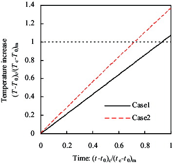
Due to uncertainty of calculated decay heat, a constant magnification number is used in the water temperature prediction system [4] during the shutdown of cooling systems, but in this validation, the magnification number was 1.0 for the decay heat. Figure 3 shows the increase of water temperature for two cases [4]. Case 1 had fuel assemblies with large decay heat which had been taken relatively recently from the shutdown reactor core and the period of cooling was short. Case 2 had fuel assemblies with small decay heat which had been taken a long time ago from the shutdown reactor core and the period of cooling was long. The air ventilation systems were operating and Equation (1) was used for evaporation heat fluxes. The maximum water temperature values were about 30 °C in Case 1 and about 40 °C in Case 2. The time and temperature were normalized by the shutdown period of the cooling systems (t_e − t₀) and temperature increase during shutdown period of the cooling systems (T_e − T₀), respectively, where t_e is the restart time of the cooling systems, t₀ is their shutdown time, T_e is the water temperature at their restart time, and T₀ is the water temperature at their shutdown time. The calculation results for Case 1 with large decay heat agreed well with measured temperatures, but the calculated water temperature increasing rate for Case 2 with small decay heat was about 35% larger than the measured temperature increasing rate. The results in Case 2 showed that the calculated decay heat was overestimated for long-time cooled fuel assemblies. Prediction of decay heat affected the water temperature and the water temperature was relatively low, so Equation (1) was not sufficiently validated.

Figure 3. Increase of water temperature during the shutdown of cooling systems.

3. Prediction of water level during loss of all AC power supplies

3.1. Prediction of water temperature

Figure 4 shows the heat transfer model used to calculate water temperature during loss of all AC power supplies. The calculation method of water temperature was the same as the method used for the shutdown of cooling systems [4], and the heat balance equation for the one-region model was used: (3) $$\begin{array}{c}\hfill C{p}_w{M}_w\left(\frac{d{T}_w}{dt}\right)=Q_D-Q_E-Q_C,\left(T_w\le 100{}^{\circ }\mathrm{C}\right)\end{array}$$(3)

Figure 4. Heat transfer model for loss of all AC power supplies.

where Cp_w (kJ/(kg·K)) is the specific heat of water, M_w (kg) is the water mass, T_w (°C) is the average water temperature, t (s) is the time after shutdown of the cooling systems or loss of all AC power supplies, Q_D (kW) is the decay heat, Q_E (kW) is the evaporation heat transfer from the water surface to air, and Q_C (kW) is the heat transfer from water to concrete. Q_C is calculated using the 1D unsteady heat conduction equation with the natural convection heat transfer correlation proposed by Kataoka et al. [10]. Q_E was calculated using the correlation of evaporation heat fluxes for natural convection air flow (Equation (2)). In Equation (3), the limitation of T_w ⩽ 100  °C automatically gives the transition from evaporation to boiling. The water surface temperature was calculated as (4) $$T_{\mathrm{ws}}=T_w-\frac{Q_E}{2C{p}_w{G}_{\mathrm{ws}}}$$(4) where T_ws (°C) is the water surface temperature and G_ws (kg/s) is the natural circulation flow rate near the water surface (hypothetical surface layer). G_ws was obtained and good agreement was seen between water temperatures (both average water temperature and water surface temperature) computed by the 3D simulation and one-region model. Then a correlation for G_ws was derived as a function of decay heat and was introduced into the prediction system with the one-region model. The fraction 1/2 in Equation (4) comes from the average of the inlet water temperature (T_w) and outlet water temperature in the hypothetical surface layer.

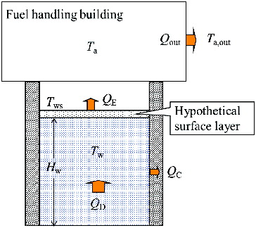
The average air temperature in the fuel handling building was calculated from enthalpy of air in the fuel handling building, which was calculated from the heat balance equation for the one-region model under the condition of 100% relative humidity: (5) $$\begin{array}{ccc}\hfill \left(\frac{d{Q}_a^{\text{'}}}{dt}\right)& =& Q_D-Q_C-C{p}_w{M}_w\left(\frac{d{T}_w}{dt}\right)-Q_{\mathrm{out}},\hfill \\ \hfill T_a& =& f\left(\frac{Q_a^{\text{'}}}{V_a}\right),\hfill \end{array}$$(5) where Q′_a (kJ) is the enthalpy of air in the fuel handling building, Q_out (kW) is the heat transfer outside the fuel handling building, T_a (°C) is the average air temperature in the fuel handling building, and V_a (m³) is the volume of the fuel handling building. The third term on the right side is the increasing rate of enthalpy of water. Q_out was calculated using a turbulent natural convection heat transfer outside of the fuel handling building neglecting effects of wind. The function f was obtained from the relationship between air temperature and its enthalpy (kJ/m³) with 100% relative humidity. Physical properties were calculated using functions of temperature. Using the term (Q_D − Q_C) instead of Q_E in Equation (5) makes it possible to calculate the heat balance after the water temperature reaches the saturated temperature of T_w = 100 °C (heat is not stored in water after boiling). Equation (5) was introduced into the water temperature prediction system [4] during shutdown of cooling systems.

3.2. Prediction of water level

The calculation method of the water level was also the same as the method for the shutdown of cooling systems [4], and the following mass balance equation for a one-region model was used: (6) $$\begin{array}{ccc}\hfill \left(\frac{d{M}_w}{dt}\right)h_{fg}& =& -\left(Q_D-Q_C\right)+C{p}_w{M}_w\left(\frac{d{T}_w}{dt}\right),\hfill \\ \hfill H_w& =& \frac{M_w}{{\rho }_w{A}_{\mathrm{ws}}},\hfill \end{array}$$(6) where H_w (m) is the water level, A_ws (m²) is the water surface area, and ρ_w (kg/m³) is the water density.

4. Validation for prediction of water temperature and level

The authors could not find any documents describing the measurement of the water temperature and level in a SFP during loss of all AC power supplies. Therefore, comparison and validation were done by using measurement results [5] in the Fukushima Daiichi Nuclear Power Station (1F) (hereafter called the 1F-Report). The objective of calculations with the one-region model for SFPs in 1F was not to reproduce the thermal-hydraulics but to validate prediction of the water temperature and the level. In 1F, some buildings were damaged and water injection was done for a long time.

In the case of a damaged building, Q_E was calculated under the condition that T_a in Figure 4 equals the outdoor temperature of T_a,out. Water injection was done periodically, but in this study, water injection was continuously assumed at the same time-averaged flow rate and subcooled heat was subtracted from Q_D in calculations of the water temperature.

4.1. Calculation conditions

Table 1 shows the calculation conditions. The initial water volume V_w,0 and initial water level H_w,0 were given in the 1F-Report [5]. The initial water temperature T_w,0, outdoor temperature, T_a,out, and temperature of injected water, T_w,in, were the same values as assumed in the 1F-Report [5].

Table 1. Calculation conditions [5].

Initial conditions
Vw,0 (m^3)	Hw,0 (m)	Tw,0 (°C)	Ta,out (°C)	Tw,in (°C)
1390	11.5	30	10	10

Note: V_w,0: initial water volume (m³), H_w,0: initial water level (m), T_w,0: initial water temperature (°C), T_a,out: outdoor temperature (°C), and T_w,in: temperature of injected water (°C).

Decay heats predicted by ORIGEN 2.2 were written for values at the beginning (t = 0) and three months later (t = 90 days) in the 1F-Report [5]. In this study, decay heat was calculated using the correlation recommended by ANS-5.1-1973 [11], in which the coefficient and index were fitted to give decay heat at t = 0, 90 days in the 1F-Report [5].

In the Unit 4 pool, water levels were measured during the no water injection periods; the calculation accuracy of decay heat was discussed by comparison of the calculated water level decreasing rate with the measured value. In the Unit 2 pool, the calculation accuracy of evaporation heat flux, during the period a high water level was kept by periodical water injection, was discussed by comparison of the calculated water temperature with the measured value.

4.2. Unit 4 pool

Decay heats in the Unit 4 SFP were reported [5] as 2.26 MW (t = 0) and 1.58 MW (t = 90 days). In the calculation for the Unit 4 pool, the water temperature and level were calculated under the conditions of the intact building and the function of the presented prediction system was considered first. Next, calculated water levels during no water injection were compared with measured values under the condition that air temperature equaled the outdoor temperature of 10 °C for the damaged building.

Figure 5 shows the calculated transient behaviors (heat gain, temperatures, water level from the top of the racks, and evaporation heat transfer coefficient) after loss of all AC power supplies with the intact building. After about three days, T_w was almost 100 °C (Figure 5(b)), Q_E rapidly increased due to boiling (Figure 5(a)), and H_w rapidly decreased (Figure 5(c)). Q_C in Figure 5(a) increased once due to the water temperature increase and then decreased due to the water level decrease and increase of T_C (Q_C was calculated for the SFP volume below the water level, not including the volume above the water level). Figure 5(b) shows that the calculated average water temperatures with and without heat losses were almost the same, because Q_D was much bigger than heat losses to concrete and air, Q_C + Q_E. T_ws values after about three days agreed well with the measured values. Water level in Figure 5(c) is the level from the top of racks. Increasing water level in the beginning was due to thermal expansion; water level without heat losses H_w,a was slightly overestimated, even though during the decreasing water level H_w,a might be generally underestimated since evaporation was ignored. Because Q_C was relatively small, calculated water levels with and without heat losses were almost the same. The calculated water level agreed well with the measured value made by visual observation from a helicopter. It took about 12.7 days until the water level decreased to the top of the racks without water injection. The calculated evaporation heat transfer coefficient in Figure 5(d) rapidly increased due to the increases in average water temperature and water surface temperature, and its value became 133 W/(m²·K) at T_ws = 87 °C. Calculated evaporation heat transfer coefficient and evaporation heat transfer rate had a significant effect on the water temperature calculation, but except for the case of small decay heat (refer to Figure 11(b)) they had only a small effect on the water level calculation.

Figure 5. Transient behavior after loss of all AC power supplies (Unit 4 pool, intact building).

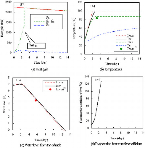
Figure 6. Transient behavior after loss of all AC power supplies (Unit 4 pool, damaged building).

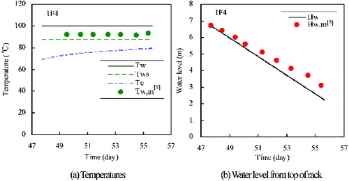
Figure 7. Water level (Unit-4 pool, damaged building, 0.8 Q_D).

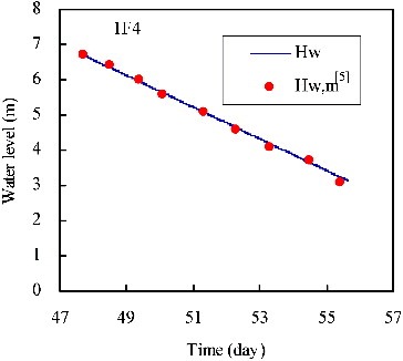
Figure 8. Transient behavior after loss of all AC power supplies (Unit 2 pool, intact building, without water injection).

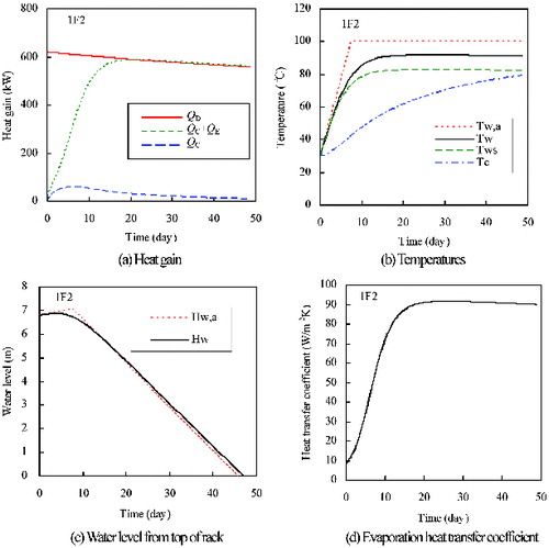
Figure 9. Transient behavior after loss of all AC power supplies (Unit 2 pool, intact building, with water injection).

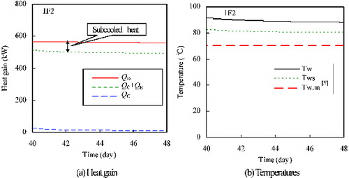
Figure 10. Effects of decay heat (Q_D) and evaporation heat flux (q_E) on water temperatures (Unit 2 pool).

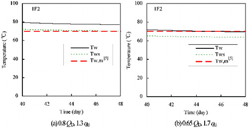
Figure 11. Effects of decay heat (Q_D) and evaporation heat flux (q_E) (Unit 2 pool, 0.8 Q_D, 2.3 q_E).

Figure 6 compares the calculation results during no water injection with measured values; the conditions were that air temperature was equal to the outdoor temperature (T_a = 10 °C) with the damaged building. Water temperature (Figure 6(a)) was measured by a thermocouple that was hung from the water injection crane, but the depth of the measuring point was not clear. The water temperature distribution by 3D calculation is necessary for estimation of the measuring point location. Measured water temperatures were between T_w and T_ws, and so water temperature calculation was considered to be reasonable. Heat transfer form was boiling (T_w = 100 °C) during this period in the calculation, and so it was hard to validate Equation (2) for evaporation heat fluxes. Calculations overestimated the decreasing rate of the water level by about 20% as shown in Figure 6(b).

The decreasing rate of the water level calculated with 80% decay heat (0.8 Q_D) agreed well with the measured value as shown in Figure 7. This showed that ORIGEN 2.2 overestimated decay heat. The same result was shown in Case 2 of Figure 3 and for this Case 2, the increasing rate of the water temperature calculated with 0.75 Q_D agreed well with the measured value.

4.3. Unit 2 pool

Decay heat in the Unit 2 pool was reported [5] as 0.62 MW (t = 0) and 0.52 MW (t = 90 days). This building was only partially damaged, so in the calculation for the Unit 2 pool, evaporation heat transfer was calculated under the condition of the intact building (evaporation heat transferred to outdoor due to discharge of mixture of steam and air in the building). Equation (2) for evaporation heat fluxes was discussed by comparison of calculated water temperatures with measured values during the period that the water level was fully kept by periodical water injection.

Figure 8 shows the calculated transient behaviors (heat gain, temperatures, water level from the top of racks, and evaporation heat transfer coefficient) under the condition of the intact building. These were almost the same behaviors as for the Unit 4 pool. Initial decay heat of the Unit 2 pool was about 27% that of the Unit 4 pool. The time until the water level decreased to the top of racks in the Unit 2 pool (Figure 8(c): about 46.6 days) took about 3.7 times longer than the time in the Unit 4 pool. Decay heat Q_D (Figure 8(a)) balanced with heat losses to concrete and air, Q_C + Q_E, at the time when the average water temperature reached about 88 °C and the water surface temperature (Figure 8(b)) was about 79 °C. Therefore, the boiling status (100 °C) was not established.

After 10 days had passed from loss of all AC power supplies, water was injected periodically, and after 40 days, the pool was evaluated as being at a high water level. Calculated results after 40 days are shown in Figure 9. In the calculations, a constant water flow was continuously assumed to keep the water level high. The temperature of the injected water was 10 °C. The difference between decay heat Q_D and heat losses to concrete and air, Q_C + Q_E, in Figure 9(a) is the subcooled heat of injected water. The measured temperatures during this period changed between about 50 and 70 °C due to the periodical water injection. Water temperature of 50 °C was evaluated as air temperature [5], i.e. a thermometer was exposed in the air due to the decrease in the water level. Maximum temperature (about 70 °C), which was evaluated as water temperature, is shown in Figure 9(b). Calculated average water temperatures and water surface temperatures were higher than measured values. The reasons for overestimating water temperature were effects of the damaged building, overestimation of decay heat, and underestimation of evaporation heat flux.

For the damaged building and the same air temperature as the outdoor temperature (T_a = 10 °C), the calculated water temperature decreased by only 4 °C–5 °C. So, the main reasons for overestimating the water temperature were overestimation of decay heat and underestimation of evaporation heat flux. In the calculation for the Unit 4 pool, the water level decreasing rate calculated with 80% decay heat (0.8Q_D) gave good agreement between the calculated and measured values. However, overestimation of water temperature could not be clarified under the calculation condition of 0.8Q_D for the Unit 2 pool.

Figure 10 shows the surveillance results of calculation conditions which gave good agreement between the calculated and measured water temperatures. Calculated water surface temperatures agreed well with measured values under the conditions of 0.8Q_D and 130% evaporation heat flux (1.3q_E) as shown in Figure 10(a). Calculated average water temperatures agreed well with measured values under the conditions of 0.65Q_D and 1.7q_E, as shown in Figure 10(b).

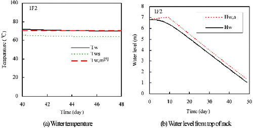
The magnification number for evaporation heat flux was 2.3 to obtain good agreement of calculated average water temperatures with measured values under the condition of 0.8Q_D, as shown in Figure 11(a). In this case, the water level calculated with heat losses to concrete and air was lower than that calculated with the adiabatic condition, as shown in Figure 11(b). Evaporation under the condition of highly subcooled water caused this early decrease in the water level. The smaller decay heat and the bigger evaporation (low water temperature) caused the lower water level. The results indicated that the adiabatic calculations were not always conservative.

4.4. Discussion

The decreasing rate of the water level was overestimated in the case of 100% decay heat (1.0Q_D) predicted by ORIGEN 2.2 (Figure 6(b)), but the deceasing rate of the water level for the 80% decay heat (0.8Q_D) predicted by ORIGEN 2.2 demonstrated good agreement with the measured water levels (Figure 7).

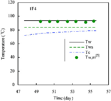
These results showed that decay heat predicted by ORIGEN 2.2 was overestimated by 25% (1/0.8 = 1.25) for long-time cooled fuel assemblies. The magnification number for evaporation heat flux was 1.55 to obtain good agreement between calculated average water temperatures and measured values under the condition of 0.8Q_D, as shown in Figure 12. This result showed that evaporation heat transfer predicted by Equation (2) was underestimated by 35% (1/1.55 = 0.65).

Figure 12. Water temperatures (Unit 4 pool, damaged building, 0.8Q_D, 1.55q_E).

Prediction error of decay heat differs according to the specifications and the status (fuel type, burn-up, cooling period, etc.) of the spent fuel assembly. If 25% overestimation of decay heat was adopted in the calculation for the Unit 2 pool, the same as for the Unit 4 pool, Equation (2) underestimated evaporation heat fluxes by 57% (1/2.3 = 0.43). Cooling time of spent fuel assemblies in the Unit 2 pool was longer than that in the Unit 4 pool; consequently, the prediction error of decay heat calculated by ORIGEN 2.2 in the Unit 2 pool would be bigger than that in the Unit 4 pool. Under the assumption that decay heat was overestimated by 54% (1/0.65 = 1.54) in the Unit 2 pool, as shown in Figure 10(b), Equation (2) underestimated evaporation heat fluxes by 41% (1/1.7 = 0.59). From these discussions, it is difficult to separate overestimation of decay heat and underestimation of evaporation heat flux quantitatively.

It was considered that the underestimation of evaporation heat flux (35%–57%) was a reasonable prediction error under the uncertainty of the correlation for turbulent natural convection heat transfer used in the derivation of Equation (2) because the measured heat gains in forced convection evaporation were about three times of the values predicted from the analogy [2].

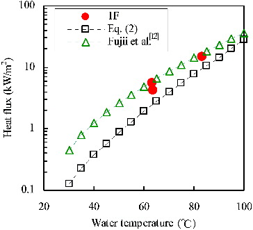
Figure 13 compares evaporation heat fluxes. The data marked as 1F in Figure 13 were calculated from the data in Figures 10(b), 11(a), and 12, and agreed well with the correlation proposed by Fujii et al. [12]. Fujii et al. measured evaporation heat fluxes with surface areas of 0.034 and 0.29 m² under pressures of 0.1–0.32 MPa in stagnant air conditions. Steam pressure ratio (P_so/P) and heat flux values of Fujii et al. were within the conditions of this study, but water temperatures (T_w ⩾ 100 °C) and steam pressure (P_so) were high. Therefore, the correlation of Fujii et al. would not be applicable to the calculation of the water temperature in the SFP. However, it is interesting that predicted evaporation heat fluxes agreed well with data-fitted evaporation heat fluxes which were adjusted with the water temperature of the Uuit 2 and Unit 4 pools. These data-fitted evaporation heat fluxes are affected by the uncertainty of the decay heat calculation. It is necessary to collect more data on evaporation heat transfer and to improve the correlation.

Figure 13. Comparison of evaporation heat fluxes.

5. Conclusions

The prediction system that was developed to predict water temperature in an SFP after the shutdown of cooling systems was extended to calculate the water level in the SFP during loss of all AC power supplies. The calculated results were validated by using the measured water temperatures and levels in SFPs at 1F. The following results were obtained:

1. The decreasing rate of the water level with decay heat predicted by ORIGEN 2.2 was overestimated. The decreasing rate of the water level calculated with 80% decay heat agreed well with measured values. These results showed that decay heat predicted by ORIGEN 2.2 was overestimated by 25% for long-time cooled fuel assemblies.

2. The correlation for evaporation heat fluxes, which was derived from the analogy between turbulent natural convection heat transfer and mass transfer of vapor, overestimated water temperatures and underestimated evaporation heat transfer by 35%–57%.

3. Evaporation heat fluxes, which were calculated to give good agreement between calculated and measured values, agreed well with the correlation proposed by Fujii et al. within limited conditions.

4. Neglect of heat losses generally had small effects on the prediction of the water level decreasing rate; however, in the case of small decay heat, the water level decreasing rate with neglect of heat losses was underestimated because enthalpy stored in water was overestimated.

References

- Collins TE, Hubbard G. Technical study of spent fuel pool accident risk at decommissioning nuclear power plants, NUREG-1738. US Nuclear Regulatory Commission (USNRC); February 2001.
- Yanagi C, Murase M, Yoshida Y, Iwaki T, Nagae T, Koizumi Y. [Evaporation heat flux form hot water to air flow]. Trans Jpn Soc Mech Eng B. February 2012;78(786):363–372. Japanese.
- Yanagi C, Murase M, Yoshida Y, Iwaki T, Nagae T. Evaluation of heat loss and water temperature in a spent fuel pit. J Power Energy Sys. June 2012;6(2):51–62.
- Yanagi C, Murase M, Yoshida Y, Iwaki T, Nagae T. [Evaluation of water temperature in spent fuel pit (5) development of a simple calculation method]. 2011 Fall Meeting of the Atomic Energy Society of Japan; 2011 September 19–22; Kitakyushu, Japan. p. 41. Japanese.
- TEPCO. Report on effects of the earthquake in the Northeastern Japan on nuclear facilities in the Fukushima Daiichi nuclear power station. The Tokyo Electric Power Company; September 2011. Japanese.
- Nuclear Safety Research Association, Tokyo, Japan. Overview of light water nuclear power stations; January 2010.
- Ludwig SB, Croff AG. Revision to ORIGEN2 – Version 2.2, Transmittal memo of CCC-0371/17. TN, USA: Oak Ridge National Laboratory; May 2002.
- Katakura J, Kataoka M, Suyama K, Jin T, Ohki S. A set of ORIGEN2 cross section libraries based on JENDL3.3 library: ORLIBJ33, JAERI-Data/Code 2004-015. Ibaragi prefecture, Japan: Japan Atomic Energy Research Institute; 2004.
- Shibata K, Kawano T, Nakagawa T, Iwamoto O, Katakura J, Fukahori T, Chiba S, Hasegawa A, Murata T, Matsunobu H, Ohsawa T, Nakajima Y, Yoshida T, Zukeran A, Kawai M, Baba M, Ishikawa M, Asami T, Watanabe T, Watanabe Y, Igashira M, Yamamuro N, Kitazawa H, Yamano N, Takano H. JENDL-3.3: Japanese evaluated nuclear data library version 3 revision-3. J Nucl Sci Technol. November 2002;39(11):1125–1136.
- Kataoka Y, Fujii T, Murase M, Tominaga K. Experimental study on heat removal characteristics for water wall type passive containment cooling system. J Nucl Sci Technol. October 1994;31(10):1043–1052.
- American Nuclear Society. Decay energy release rates following shutdown of uranium-cooled thermal reactors. IL, USA: American Nuclear Society; 1973. ANS-5.1-1973.
- Fujii T, Kataoka Y, Murase M. Evaporation and condensation heat transfer in a suppression chamber of the water wall type passive containment cooling system. J Nucl Sci Technol. May 1996;33(5):374–380.