Sub-cell balanced nodal expansion methods using S₄ eigenfunctions for multi-group S_N transport problems in slab geometry

Abstract

A highly accurate S₄ eigenfunction-based nodal method has been developed to solve multi-group discrete ordinate neutral particle transport problems with a linearly anisotropic scattering in slab geometry. The new method solves the even-parity form of discrete ordinates transport equation with an arbitrary S_N order angular quadrature using two sub-cell balance equations and the S₄ eigenfunctions of within-group transport equation. The four eigenfunctions from S₄ approximation have been chosen as basis functions for the spatial expansion of the angular flux in each mesh. The constant and cubic polynomial approximations are adopted for the scattering source terms from other energy groups and fission source. A nodal method using the conventional polynomial expansion and the sub-cell balances was also developed to be used for demonstrating the high accuracy of the new methods. Using the new methods, a multi-group eigenvalue problem has been solved as well as fixed source problems. The numerical test results of one-group problem show that the new method has third-order accuracy as mesh size is finely refined and it has much higher accuracies for large meshes than the diamond differencing method and the nodal method using sub-cell balances and polynomial expansion of angular flux. For multi-group problems including eigenvalue problem, it was demonstrated that the new method using the cubic polynomial approximation of the sources could produce very accurate solutions even with large mesh sizes.

Keywords:

• discrete ordinates method
• eigenfunction expansion
• sub-cell balances

1. Introduction

The accurate solutions of the transport equation are important in many engineering areas such as nuclear reactor design, radiation shielding, optical tomography, and radiative transfer problems. It has been well known that the transport equation is quite difficult to solve analytically even for slab geometry problems except for very simple cases. Hence, there have been tremendous studies on developing accurate numerical differencing schemes for the Boltzmann transport equation [1–5]. In slab geometry problem, a steady-state transport equation has three independent variables: the spatial position, the directional cosine, and the energy of the particle. Typically, the dependency of the angular flux on energy is discretized by the multi-group approximation that divides the whole energy range into a finite number of discrete energy intervals [1–3]. One of the most direct and powerful methods to approximate the angular variables is the discrete ordinates method [1–4]. In the S_N method, the angular variable is discretized into a finite number of discrete directions, and the transport equation is solved for these discrete directions. For the first-order form of multi-group discrete ordinates transport equation, the exact spatial discretization methods that can give exact solutions with no truncation errors have already been developed [6–9]. These methods require a complete set of eigenfunctions of the given problem. However, finding the complete set of eigenfunctions is usually very difficult for such problems as requiring high-order angular resolution and many energy groups. On the other hand, there has been great success in the development of eigenfunction expansion method in the area of multi-group neutron diffusion theory [10].

In this paper, a new advanced method which can produce highly accurate solutions for multi-group transport equation in slab geometry problems has been developed. The second-order form, i.e., even-parity form [1,2] is considered rather than the first-order form of the transport equation in order to exploit the similarity of equation form to the neutron diffusion equation. Author's earlier works for one-group problems were presented only in the conferences (i.e., [11] and [12] for isotropic source and linearly anisotropic source problems, respectively). The previous works [11,12] showed that our new method using S₄ eigenfunction expansion and sub-cell balances gives extremely accurate solutions irrespective of mesh sizes (i.e., almost no truncation error). The present work in this paper extends the idea to multi-group problems and it also includes one-group test results for checking the order of convergence of new method as mesh size is finely refined. In this method, the sub-cell balance approaches [13–16] and the eigenfunction expansion method [6–8,10] are consistently combined for the coupling equations of unknowns. The angular fluxes are expanded using four eigenfunctions of the S₄ within-group transport equation. The unknowns in this new method are two sub-cell average angular fluxes and two edge angular fluxes of each mesh. The four expansion coefficients are coupled by two sub-cell balance conditions and two continuity conditions of odd-parity angular fluxes. In case of one-group problems, only approximation in this new method is the adaptation of the four S₄ eigenfunctions rather than exact eigenfunctions of the discrete ordinates transport equation. The reason for using the four eigenfunctions of the S₄ within-group transport equation rather than the full set of the eigenfunctions of the multi-group S_N transport equation is to avoid the complicated computation of the full set of the exact eigenvalues and the corresponding eigenfunctions because it is required to compose (N × G) × (N × G) matrix equation for each material region with the full eigenvalues and eigenfunctions of the multi-group S_N transport equation and also complex eigenvalues can be occurred for eigenvalue problems. Another reason is to limit the number of expansion terms (i.e., number of nodal knowns) to a fixed number for all the problems including multi-group problems and for an arbitrary order of angular quadrature set. This point is the key of our method. It is clear that the new eigenfunction expansion method gives the exact solution without truncation error when the one-group transport equation is solved with the S₄ angular quadrature set but produces approximate solutions when used with higher order S_N quadrature even for one-group problems. In case of multi-group problems, the eigenfunction expansion method requires additional approximation on the scattering and fission sources because the eigenfunctions of a within-group transport equation is used rather than the eigenfunctions of fully coupled multi-group transport equation. In this paper, two types of approximations of the scattering source terms from other groups including fission source have been considered to analyze the effects of the spatial shape approximation for the scattering sources from other groups including fission source on the accuracy: (1) cubic polynomial spatial distribution and (2) constant spatial distribution. The sub-cell balance method with these approximations combined with S₄ eigenfunction expansion are denoted as SCB-EEM1 (cubic) and SCB-EEM2 (constant), respectively. In addition, a sub-cell balance method with a polynomial expansion of angular flux was also newly developed to show the effects of different expansion methods on the accuracy and this method is denoted as SCB-PEM. The SCB-PEM does not require any explicit approximation of source terms. These new methods were applied to solve various test problems including eigenvalue problems as well as fixed source problems.

This paper is organized as follows. Chapter 2 provides an introduction to multi-group even-parity transport equation with discrete ordinates approximation in slab geometry, its spectral analysis, and the derivation of new eigenfunction expansion methods. The numerical tests and analyses will be given in Chapter 3. Chapter 4 will conclude this paper.

2. Methodology

2.1. Spectral analysis of within-group even-parity transport equation

We start with the following multi-group even-parity transport equation of second-order form considering linearly anisotropic scattering [1,11,12]: (1) $$\begin{array}{c}-{\mu }^2\frac{\partial }{\partial x}\left(\frac{1}{{\sigma }_g}\frac{\partial {\psi }_g^{+}}{\partial x}\right)+{\sigma }_g{\psi }_g^{+}(x,\mu )={\sigma }_{s0,g\to g}{\phi }_g\left(x\right)\hfill \\ -3{\mu }^2{c}_{s1,g\to g}\frac{\partial J_g\left(x\right)}{\partial x}+s_g\left(x\right)+\sum _{g^{\text{'}}\ne g}{\sigma }_{s0,g^{\text{'}}\to g}{\phi }_{g^{\text{'}}}\left(x\right)\hfill \\ -3{\mu }^2\sum _{g^{\text{'}}\ne g}{c}_{s1,g^{\text{'}}\to g}\frac{\partial J_{g^{\text{'}}}\left(x\right)}{\partial x},\hfill \end{array}$$(1) where ψ⁺_g(x, μ) means the even-parity angular flux for energy group g and direction μ, and φ_g(x) is the scalar flux, and J_g(x) is the net current. In Equation (1(1) $$\begin{array}{c}-{\mu }^2\frac{\partial }{\partial x}\left(\frac{1}{{\sigma }_g}\frac{\partial {\psi }_g^{+}}{\partial x}\right)+{\sigma }_g{\psi }_g^{+}(x,\mu )={\sigma }_{s0,g\to g}{\phi }_g\left(x\right)\hfill \\ -3{\mu }^2{c}_{s1,g\to g}\frac{\partial J_g\left(x\right)}{\partial x}+s_g\left(x\right)+\sum _{g^{\text{'}}\ne g}{\sigma }_{s0,g^{\text{'}}\to g}{\phi }_{g^{\text{'}}}\left(x\right)\hfill \\ -3{\mu }^2\sum _{g^{\text{'}}\ne g}{c}_{s1,g^{\text{'}}\to g}\frac{\partial J_{g^{\text{'}}}\left(x\right)}{\partial x},\hfill \end{array}$$(1) ), c_{s1, g′ → g} is the linearly anisotropic scattering ratio which is defined as the ratio of the linearly anisotropic scattering cross section (σ_{s1, g′ → g}) to the total cross section (σ_g), and the other notations are conventional ones. Next, the discrete ordinate approximation with the Gauss–Legendre quadrature [1] is applied to Equation (1(1) $$\begin{array}{c}-{\mu }^2\frac{\partial }{\partial x}\left(\frac{1}{{\sigma }_g}\frac{\partial {\psi }_g^{+}}{\partial x}\right)+{\sigma }_g{\psi }_g^{+}(x,\mu )={\sigma }_{s0,g\to g}{\phi }_g\left(x\right)\hfill \\ -3{\mu }^2{c}_{s1,g\to g}\frac{\partial J_g\left(x\right)}{\partial x}+s_g\left(x\right)+\sum _{g^{\text{'}}\ne g}{\sigma }_{s0,g^{\text{'}}\to g}{\phi }_{g^{\text{'}}}\left(x\right)\hfill \\ -3{\mu }^2\sum _{g^{\text{'}}\ne g}{c}_{s1,g^{\text{'}}\to g}\frac{\partial J_{g^{\text{'}}}\left(x\right)}{\partial x},\hfill \end{array}$$(1) ), which leads to (2) $$\begin{array}{c}-{\mu }_m^2\frac{\partial }{\partial x}\left(\frac{1}{{\sigma }_g}\frac{\partial {\psi }_{g,m}^{+}}{\partial x}\right)+{\sigma }_g{\psi }_{g,m}^{+}\left(x\right)={\sigma }_{s0,g\to g}{\phi }_g\left(x\right)\hfill \\ -3{\mu }_m^2{c}_{s1,g\to g}\frac{\partial J_g\left(x\right)}{\partial x}+s_g\left(x\right)+\sum _{g^{\text{'}}\ne g}{\sigma }_{s0,g^{\text{'}}\to g}{\phi }_{g^{\text{'}}}\left(x\right)\hfill \\ -3{\mu }_m^2\sum _{g^{\text{'}}\ne g}{c}_{s1,g^{\text{'}}\to g}\frac{\partial J_{g^{\text{'}}}\left(x\right)}{\partial x},\hfill \end{array}$$(2) where the subscript m denotes the discrete ordinate direction, and the scalar flux and current are approximated using the Gauss–Legendre quadrature, which are given by (3) $$\begin{array}{ccc}\hfill \phi \left(x\right)& =& \frac{1}{2}{\int }_{-1}^{1}d\mu \psi (x,\mu )={\int }_0^{1}d\mu {\psi }^{+}(x,\mu )\hfill \\ =& \sum _{m=1}^{N/2}{w}_m{\psi }_m^{+}\left(x\right),\hfill \\ \hfill J\left(x\right)& =& \frac{1}{2}{\int }_{-1}^{1}d\mu \mu \psi (x,\mu )={\int }_0^{1}d\mu \mu {\psi }^{-}(x,\mu )\hfill \\ =& \sum _{m=1}^{N/2}{w}_m{\mu }_m{\psi }_m^{-}\left(x\right),\hfill \end{array}$$(3) where the weights w_m are normalized such that their sum is 2.0. In Equation (3(3) $$\begin{array}{ccc}\hfill \phi \left(x\right)& =& \frac{1}{2}{\int }_{-1}^{1}d\mu \psi (x,\mu )={\int }_0^{1}d\mu {\psi }^{+}(x,\mu )\hfill \\ =& \sum _{m=1}^{N/2}{w}_m{\psi }_m^{+}\left(x\right),\hfill \\ \hfill J\left(x\right)& =& \frac{1}{2}{\int }_{-1}^{1}d\mu \mu \psi (x,\mu )={\int }_0^{1}d\mu \mu {\psi }^{-}(x,\mu )\hfill \\ =& \sum _{m=1}^{N/2}{w}_m{\mu }_m{\psi }_m^{-}\left(x\right),\hfill \end{array}$$(3) ), N means the total number of discrete ordinate directions (i.e., the order of S_N angular quadrature). From Equation (3(3) $$\begin{array}{ccc}\hfill \phi \left(x\right)& =& \frac{1}{2}{\int }_{-1}^{1}d\mu \psi (x,\mu )={\int }_0^{1}d\mu {\psi }^{+}(x,\mu )\hfill \\ =& \sum _{m=1}^{N/2}{w}_m{\psi }_m^{+}\left(x\right),\hfill \\ \hfill J\left(x\right)& =& \frac{1}{2}{\int }_{-1}^{1}d\mu \mu \psi (x,\mu )={\int }_0^{1}d\mu \mu {\psi }^{-}(x,\mu )\hfill \\ =& \sum _{m=1}^{N/2}{w}_m{\mu }_m{\psi }_m^{-}\left(x\right),\hfill \end{array}$$(3) ), it is noted that the consideration of the particles with only positive directional cosines is sufficient to calculate the angular flux moments with the even-parity formulation. With the even-parity formulation, the neutron net current is given by [1,12] (4) $$\begin{array}{ccc}\hfill J_g\left(x\right)& =& \frac{1}{1-c_{s1,g\to g}\left(x\right)}[-\frac{1}{{\sigma }_g}\frac{\partial }{\partial x}\sum _{m=1}^{N/2}{w}_m{\mu }_m^2{\psi }_g^{+}(x,{\mu }_m)\hfill \\ +\sum _{g^{\text{'}}\ne g}{c}_{s1,g^{\text{'}}\to g}{J}_{g^{\text{'}}}\left(x\right)],\hfill \end{array}$$(4)

In our new methods, the four eigenfunctions of the within-group even-parity transport equation with S₄ approximation are used as the expansion basis functions for the homogeneous angular flux while the spatial distribution of the scattering sources from other energy groups and fission source are approximated to be either constant or cubic polynomial shape. This simplification is to avoid the complexities of finding the eigenvalues and eigenfunctions of the fully coupled multi-group S_N transport equation. The homogeneous form of the within-group even-parity transport equations are obtained by removing the scattering source terms from other groups and external source in Equations (2) and (4). The resulting equations are given by (5) $$\begin{array}{c}-{\mu }_m^2\frac{\partial }{\partial x}\left(\frac{1}{{\sigma }_g}\frac{\partial {\psi }_{g,m}^{+,h}}{\partial x}\right)+{\sigma }_g{\psi }_{g,m}^{+,h}\left(x\right)={\sigma }_{s0,g\to g}{\phi }_g^h\left(x\right)\hfill \\ -3{\mu }_m^2{c}_{s1,g\to g}\frac{\partial J_g^h\left(x\right)}{\partial x},\hfill \\ J_g^h\left(x\right)=\frac{-1}{1-c_{s1,g\to g}}\frac{1}{{\sigma }_g}\frac{\partial }{\partial x}\sum _{n=1}^{N/2}{w}_n{\mu }_n^2{\psi }_{g,n}^{+,h}\left(x\right),\hfill \end{array}$$(5) where ψ ^{+, h}_{g, m}(x) is the homogeneous even-parity angular flux. Next, the ansatz of the following form [6,7] is used: (6) $${\psi }_{g,m}^{+,h}\left(x\right)=a_{g,m}\left(\nu \right)e^{-{\sigma }_{g}x/\nu },$$(6) where ν and a_{g, m}(ν) are an eigenvalue and its corresponding vector, respectively. Then, the substitution of Equation (6(6) $${\psi }_{g,m}^{+,h}\left(x\right)=a_{g,m}\left(\nu \right)e^{-{\sigma }_{g}x/\nu },$$(6) ) into Equation (5(5) $$\begin{array}{c}-{\mu }_m^2\frac{\partial }{\partial x}\left(\frac{1}{{\sigma }_g}\frac{\partial {\psi }_{g,m}^{+,h}}{\partial x}\right)+{\sigma }_g{\psi }_{g,m}^{+,h}\left(x\right)={\sigma }_{s0,g\to g}{\phi }_g^h\left(x\right)\hfill \\ -3{\mu }_m^2{c}_{s1,g\to g}\frac{\partial J_g^h\left(x\right)}{\partial x},\hfill \\ J_g^h\left(x\right)=\frac{-1}{1-c_{s1,g\to g}}\frac{1}{{\sigma }_g}\frac{\partial }{\partial x}\sum _{n=1}^{N/2}{w}_n{\mu }_n^2{\psi }_{g,n}^{+,h}\left(x\right),\hfill \end{array}$$(5) ) leads to (7) $$\begin{array}{c}\left[-\frac{{\mu }_m^2}{{\nu }^2}+1\right]a_{g,m}\left(\nu \right)\hfill \\ =c_{s0,g\to g}\sum _{n=1}^{N/2}{w}_n{a}_{g,n}\left(\nu \right)\hfill \\ +3{\mu }_m^2\frac{c_{s1,g\to g}}{(1-c_{s1,g\to g}){\nu }^2}\sum _{n=1}^{N/2}{w}_n{\mu }_n^2{a}_{g,n}\left(\nu \right).\hfill \end{array}$$(7) where c_{s0, g → g} is the ratio of the isotropic scattering cross section (σ_{s0, g → g}) to the total cross section (σ_g).

At this point, the eigenvectors are normalized such that they satisfy the following condition: (8) $$\sum _{m=1}^{N/2}{w}_m{a}_{g,m}\left(\nu \right)=1.$$(8)

With this normalization, the summation of Equation (7(7) $$\begin{array}{c}\left[-\frac{{\mu }_m^2}{{\nu }^2}+1\right]a_{g,m}\left(\nu \right)\hfill \\ =c_{s0,g\to g}\sum _{n=1}^{N/2}{w}_n{a}_{g,n}\left(\nu \right)\hfill \\ +3{\mu }_m^2\frac{c_{s1,g\to g}}{(1-c_{s1,g\to g}){\nu }^2}\sum _{n=1}^{N/2}{w}_n{\mu }_n^2{a}_{g,n}\left(\nu \right).\hfill \end{array}$$(7) ) over the discrete directions after multiplying it with the weight w_m gives (9) $$\sum _{m=1}^{N/2}{w}_m{\mu }_m^2{a}_{g,m}\left(\nu \right)=(1-c_{s0,g\to g})(1-c_{s1,g\to g}){\nu }^2.$$(9)

So, the formula for the eigenfunction is finally obtained, which is given by (10) $$a_{g,m}\left(\nu \right)=\frac{c_{s0,g\to g}+3{\mu }_m^2{c}_{s1,g\to g}(1-c_{s0,g\to g})}{1-\frac{{\mu }_m^2}{{\nu }^2}}.$$(10)

This formula for the eigenfunction is exactly the same as that of the first-order form of the one-group transport equation with the discrete ordinate approximation [6,7]. The eigenvalues are determined by Equations (8) and (10). Also, it is well known that the eigenvalues are all real and they are distributed symmetrically around zero if the isotropic and linearly anisotropic scattering ratios are less than unity [6]. Although there are N eigenvalues for each energy group, our methods need only four eigenfunctions because the even-parity angular flux will be expanded with only four terms. In author's earlier study, two methods of the eigenfunction selection were analyzed for one-group problems [11,12]. The first method was to select two eigenfunctions corresponding to the two largest positive eigenvalues and two eigenfuctions corresponding to negative eigenvalues of the same absolute values as the two largest positive eigenvalues, while the second method selected the four eigenfunctions of the discrete ordinates transport equation with S₄ approximation. The previous studies [11,12] showed that the latter selection method gives more accurate solutions for various one-group problems. Consequently, in this paper, the four eigenfunctions of the within-group S₄ transport equation were used as the basis functions for the expansion of even-parity angular flux.

2.2. Eigenfunction expansion method

As mentioned in the previous section, the four eigenfunctions of the within-group S₄ discrete ordinates even-parity transport equation will be used to approximate the spatial shape homogeneous even-parity angular flux of arbitrary S_N angular quadrature. Now, it is needed to find the particular even-parity angular flux to construct the total even-parity angular flux. As mentioned in Chapter 1, the sum of scattering source from other groups and fission source was considered as the external sources, and the spatial shape of these external sources needs to be approximated to determine the spatial shape of the particular even-parity angular flux. Before proceeding to further derivation, the multi-group even-parity transport equation, Equation (2(2) $$\begin{array}{c}-{\mu }_m^2\frac{\partial }{\partial x}\left(\frac{1}{{\sigma }_g}\frac{\partial {\psi }_{g,m}^{+}}{\partial x}\right)+{\sigma }_g{\psi }_{g,m}^{+}\left(x\right)={\sigma }_{s0,g\to g}{\phi }_g\left(x\right)\hfill \\ -3{\mu }_m^2{c}_{s1,g\to g}\frac{\partial J_g\left(x\right)}{\partial x}+s_g\left(x\right)+\sum _{g^{\text{'}}\ne g}{\sigma }_{s0,g^{\text{'}}\to g}{\phi }_{g^{\text{'}}}\left(x\right)\hfill \\ -3{\mu }_m^2\sum _{g^{\text{'}}\ne g}{c}_{s1,g^{\text{'}}\to g}\frac{\partial J_{g^{\text{'}}}\left(x\right)}{\partial x},\hfill \end{array}$$(2) ), is rewritten as follows: (11) $$\begin{array}{c}-{\mu }_m^2\frac{\partial }{\partial x}\left(\frac{1}{{\sigma }_g}\frac{\partial {\psi }_{g,m}^{+}}{\partial x}\right)+{\sigma }_g{\psi }_{g,m}^{+}\left(x\right)={\sigma }_{s0,g\to g}{\phi }_g\left(x\right)\hfill \\ -3{\mu }_m^2{c}_{s1,g\to g}\frac{\partial J_g\left(x\right)}{\partial x}+q_{g,m}\left(x\right),\hfill \\ q_{g,m}\left(x\right)=s_g\left(x\right)+\sum _{g^{\text{'}}\ne g}{\sigma }_{s0,g^{\text{'}}\to g}{\phi }_{g^{\text{'}}}\left(x\right)\hfill \\ -3{\mu }_m^2\sum _{g^{\text{'}}\ne g}{c}_{s1,g^{\text{'}}\to g}\frac{\partial J_{g^{\text{'}}}\left(x\right)}{\partial x}.\hfill \end{array}$$(11)

Approximations of the cubic and quadratic shapes have been made for the scalar fluxes and currents, respectively, in the scattering from other groups and fission source terms in each mesh, which is referred to as SCB-EEM1 in this paper. The coefficients of this polynomial approximation of scalar fluxes can be calculated as follows by preserving the sub-cell average scalar fluxes and the scalar fluxes at the mesh edges: (12) $$\begin{array}{ccc}\hfill {\varphi }_g\left(x\right)& =& A_{g,i}+B_{g,i}x+C_{g,i}{x}^2+D_{g,i}{x}^3,\hfill \\ \hfill A_{g,i}& =& \frac{3}{4}({\varphi }_{g,i,hl}+{\varphi }_{g,i,hr})-\frac{1}{4}({\varphi }_{g,i}+{\varphi }_{g,i+1}),\hfill \\ \hfill B_{g,i}& =& \frac{4}{h}({\varphi }_{g,i,hr}-{\varphi }_{g,i,hl})-\frac{1}{h}({\varphi }_{g,i+1}-{\varphi }_{g,i}),\hfill \\ \hfill C_{g,i}& =& \frac{3}{h^2}[{\varphi }_{g,i+1}+{\varphi }_{g,i}-({\varphi }_{g,i,hl}+{\varphi }_{g,i,hr})],\hfill \\ \mathrm{and}\hfill \\ \hfill D_{g,i}& =& \frac{8}{h^3}({\varphi }_{g,i+1}+{\varphi }_{g,i})-\frac{16}{h^3}({\varphi }_{g,i,hr}-{\varphi }_{g,i,hl}),\hfill \end{array}$$(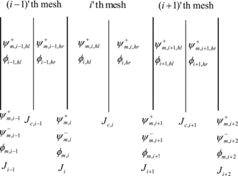12) where φ_{g, i, hl} and φ_{g, i, hr} are the sub-cell average scalar fluxes over the left-half and the right-half sub-cells of the ith mesh, respectively, while φ_{g, i} is the scalar flux at the left edge of the ith mesh, and h is the mesh width. For each mesh, the origin of x-coordinate is at the center of mesh. Figure 1 shows the mesh and sub-cell divisions including the unknowns which are used in the derivations. In Figure 1, the subscript g for the current and fluxes is omitted for simplicity.

Figure 1. Meshes, sub-cell divisions, and unknown variables.

On the other hand, the neutron currents in the linearly anisotropic scattering source terms are assumed to be quadratic spatial shape and their coefficients can be determined by preserving the currents at the edges and at the center of mesh as follows: (13) $$\begin{array}{ccc}\hfill J_g\left(x\right)& =& E_{g,i}+F_{g,i}x+G_{g,i}{x}^2,\hfill \\ \hfill E_{g,i}& =& J_{c,g,i},\hfill \\ \hfill F_{g,i}& =& \frac{J_{g,i+1}-J_{g,i}}{h},\hfill \\ \hfill G_{g,i}& =& \frac{2}{h^2}[J_{g,i+1}+J_{g,i}-2J_{c,g,i}].\hfill \end{array}$$(13)

Next, removing the neutron current term of the energy group g in Equation (11(11) $$\begin{array}{c}-{\mu }_m^2\frac{\partial }{\partial x}\left(\frac{1}{{\sigma }_g}\frac{\partial {\psi }_{g,m}^{+}}{\partial x}\right)+{\sigma }_g{\psi }_{g,m}^{+}\left(x\right)={\sigma }_{s0,g\to g}{\phi }_g\left(x\right)\hfill \\ -3{\mu }_m^2{c}_{s1,g\to g}\frac{\partial J_g\left(x\right)}{\partial x}+q_{g,m}\left(x\right),\hfill \\ q_{g,m}\left(x\right)=s_g\left(x\right)+\sum _{g^{\text{'}}\ne g}{\sigma }_{s0,g^{\text{'}}\to g}{\phi }_{g^{\text{'}}}\left(x\right)\hfill \\ -3{\mu }_m^2\sum _{g^{\text{'}}\ne g}{c}_{s1,g^{\text{'}}\to g}\frac{\partial J_{g^{\text{'}}}\left(x\right)}{\partial x}.\hfill \end{array}$$(11) ) using Equation (4(4) $$\begin{array}{ccc}\hfill J_g\left(x\right)& =& \frac{1}{1-c_{s1,g\to g}\left(x\right)}[-\frac{1}{{\sigma }_g}\frac{\partial }{\partial x}\sum _{m=1}^{N/2}{w}_m{\mu }_m^2{\psi }_g^{+}(x,{\mu }_m)\hfill \\ +\sum _{g^{\text{'}}\ne g}{c}_{s1,g^{\text{'}}\to g}{J}_{g^{\text{'}}}\left(x\right)],\hfill \end{array}$$(4) ) leads to the following equation: (14) $$\begin{array}{c}-{\mu }_m^2\frac{\partial }{\partial x}\left(\frac{1}{{\sigma }_g}\frac{\partial {\psi }_{g,m}^{+}}{\partial x}\right)+{\sigma }_g{\psi }_{g,m}^{+}\left(x\right)={\sigma }_{s0,g\to g}\sum _{n=1}^{N/2}{w}_n{\psi }_{g,n}^{+}\hfill \\ +\frac{3{\mu }_m^2{c}_{s1,g\to g}}{(1-c_{s1,g\to g}){\sigma }_g}\sum _{n=1}^{N/2}{w}_n{\mu }_n^2\frac{{\partial }^2{\psi }_{g,n}^{+}}{\partial x^2}+q_{g,m}\left(x\right),\hfill \\ q_{g,m}\left(x\right)=s_g\left(x\right)+\sum _{g^{\text{'}}\ne g}{\sigma }_{s0,g^{\text{'}}\to g}[A_{g^{\text{'}}}+B_{g^{\text{'}}}x+C_{g^{\text{'}}}{x}^2+D_{g^{\text{'}}}{x}^3]\hfill \\ -\frac{3{\mu }_m^2}{1-c_{s1,g\to g}}\sum _{g^{\text{'}}\ne g}{c}_{s1,g^{\text{'}}\to g}[F_{g^{\text{'}}}+2G_{g^{\text{'}}}x].\hfill \end{array}$$(14)

In Equation (14(14) $$\begin{array}{c}-{\mu }_m^2\frac{\partial }{\partial x}\left(\frac{1}{{\sigma }_g}\frac{\partial {\psi }_{g,m}^{+}}{\partial x}\right)+{\sigma }_g{\psi }_{g,m}^{+}\left(x\right)={\sigma }_{s0,g\to g}\sum _{n=1}^{N/2}{w}_n{\psi }_{g,n}^{+}\hfill \\ +\frac{3{\mu }_m^2{c}_{s1,g\to g}}{(1-c_{s1,g\to g}){\sigma }_g}\sum _{n=1}^{N/2}{w}_n{\mu }_n^2\frac{{\partial }^2{\psi }_{g,n}^{+}}{\partial x^2}+q_{g,m}\left(x\right),\hfill \\ q_{g,m}\left(x\right)=s_g\left(x\right)+\sum _{g^{\text{'}}\ne g}{\sigma }_{s0,g^{\text{'}}\to g}[A_{g^{\text{'}}}+B_{g^{\text{'}}}x+C_{g^{\text{'}}}{x}^2+D_{g^{\text{'}}}{x}^3]\hfill \\ -\frac{3{\mu }_m^2}{1-c_{s1,g\to g}}\sum _{g^{\text{'}}\ne g}{c}_{s1,g^{\text{'}}\to g}[F_{g^{\text{'}}}+2G_{g^{\text{'}}}x].\hfill \end{array}$$(14) ), the spatial shapes of scalar flux and currents in Equations (12) and (13) have been introduced into the source term. As shown in Equation (14(14) $$\begin{array}{c}-{\mu }_m^2\frac{\partial }{\partial x}\left(\frac{1}{{\sigma }_g}\frac{\partial {\psi }_{g,m}^{+}}{\partial x}\right)+{\sigma }_g{\psi }_{g,m}^{+}\left(x\right)={\sigma }_{s0,g\to g}\sum _{n=1}^{N/2}{w}_n{\psi }_{g,n}^{+}\hfill \\ +\frac{3{\mu }_m^2{c}_{s1,g\to g}}{(1-c_{s1,g\to g}){\sigma }_g}\sum _{n=1}^{N/2}{w}_n{\mu }_n^2\frac{{\partial }^2{\psi }_{g,n}^{+}}{\partial x^2}+q_{g,m}\left(x\right),\hfill \\ q_{g,m}\left(x\right)=s_g\left(x\right)+\sum _{g^{\text{'}}\ne g}{\sigma }_{s0,g^{\text{'}}\to g}[A_{g^{\text{'}}}+B_{g^{\text{'}}}x+C_{g^{\text{'}}}{x}^2+D_{g^{\text{'}}}{x}^3]\hfill \\ -\frac{3{\mu }_m^2}{1-c_{s1,g\to g}}\sum _{g^{\text{'}}\ne g}{c}_{s1,g^{\text{'}}\to g}[F_{g^{\text{'}}}+2G_{g^{\text{'}}}x].\hfill \end{array}$$(14) ), the total source term is represented by the cubic spatial distribution. If the problem is a fixed source problem, the external source is approximated to be spatially flat while the fission source is approximated to be spatially cubic as follows: (15) $$s_{f,g}\left(x\right)=\frac{1}{k_{\mathrm{eff}}}\sum _{g^{\text{'}}=1}^G\nu {\sigma }_{f{g}^{\text{'}}}[A_{g^{\text{'}}}+B_{g^{\text{'}}}x+C_{g^{\text{'}}}{x}^2+D_{g^{\text{'}}}{x}^3].$$(15)

Hence, the cubic spatial distribution of the particular even-parity angular flux can be written as follows: (16) $${\psi }_{g,m}^{+,p}\left(x\right)={\alpha }_{g,m}+{\beta }_{g,m}x+{\gamma }_{g,m}{x}^2+{\delta }_{g,m}{x}^3.$$(16)

The coefficients of Equation (16(16) $${\psi }_{g,m}^{+,p}\left(x\right)={\alpha }_{g,m}+{\beta }_{g,m}x+{\gamma }_{g,m}{x}^2+{\delta }_{g,m}{x}^3.$$(16) ) are determined by substituting Equation (16(16) $${\psi }_{g,m}^{+,p}\left(x\right)={\alpha }_{g,m}+{\beta }_{g,m}x+{\gamma }_{g,m}{x}^2+{\delta }_{g,m}{x}^3.$$(16) ) into Equation (14(14) $$\begin{array}{c}-{\mu }_m^2\frac{\partial }{\partial x}\left(\frac{1}{{\sigma }_g}\frac{\partial {\psi }_{g,m}^{+}}{\partial x}\right)+{\sigma }_g{\psi }_{g,m}^{+}\left(x\right)={\sigma }_{s0,g\to g}\sum _{n=1}^{N/2}{w}_n{\psi }_{g,n}^{+}\hfill \\ +\frac{3{\mu }_m^2{c}_{s1,g\to g}}{(1-c_{s1,g\to g}){\sigma }_g}\sum _{n=1}^{N/2}{w}_n{\mu }_n^2\frac{{\partial }^2{\psi }_{g,n}^{+}}{\partial x^2}+q_{g,m}\left(x\right),\hfill \\ q_{g,m}\left(x\right)=s_g\left(x\right)+\sum _{g^{\text{'}}\ne g}{\sigma }_{s0,g^{\text{'}}\to g}[A_{g^{\text{'}}}+B_{g^{\text{'}}}x+C_{g^{\text{'}}}{x}^2+D_{g^{\text{'}}}{x}^3]\hfill \\ -\frac{3{\mu }_m^2}{1-c_{s1,g\to g}}\sum _{g^{\text{'}}\ne g}{c}_{s1,g^{\text{'}}\to g}[F_{g^{\text{'}}}+2G_{g^{\text{'}}}x].\hfill \end{array}$$(14) ) and then comparing the coefficients of the resulting equations. The explicit formulas for these coefficients are written as (17) $$\begin{array}{ccc}\hfill {\delta }_{g,m}& =& {\delta }_g=\frac{1}{1-c_{s0,g\to g}}\sum _{g^{\text{'}}\ne g}{c}_{s0,g^{\text{'}}\to g}{D}_{g^{\text{'}}},\hfill \\ \hfill {\gamma }_{g,m}& =& {\gamma }_g=\frac{1}{1-c_{s0,g\to g}}\sum _{g^{\text{'}}\ne g}{c}_{s0,g^{\text{'}}\to g}{C}_{g^{\text{'}}},\hfill \\ \hfill {\beta }_g& =& \frac{1}{{\sigma }_g-{\sigma }_{s0,g\to g}}[\frac{2}{{\sigma }_g}\frac{{\delta }_g}{1-c_{s1,g\to g}}+\sum _{g^{\text{'}}\ne g}{\sigma }_{s0,g^{\text{'}}\to g}{B}_{g^{\text{'}}}\hfill \\ -\frac{2}{1-c_{s1,g\to g}}\sum _{g^{\text{'}}\ne g}{c}_{s1,g^{\text{'}}\to g}{G}_{g^{\text{'}}}],\hfill \\ \hfill {\beta }_{g,m}& =& c_{s0,g\to g}{\beta }_g+\sum _{g^{\text{'}}\ne g}{c}_{s0,g^{\text{'}}\to g}{B}_{g^{\text{'}}}\hfill \\ +\frac{6{\mu }_m^2}{(1-c_{s1,g\to g}){\sigma }_g}\left[\frac{1}{{\sigma }_g}{\delta }_g-\sum _{g^{\text{'}}\ne g}{c}_{s1,g^{\text{'}}\to g}{G}_{g^{\text{'}}}\right],\hfill \\ \hfill {\alpha }_g& =& \frac{1}{{\sigma }_g-{\sigma }_{s0,g\to g}}[\frac{2}{3}\frac{{\gamma }_g}{(1-c_{s1,g\to g}){\sigma }_g}+s_g\hfill \\ +\sum _{g^{\text{'}}\ne g}{\sigma }_{s0,g^{\text{'}}\to g}{A}_{g^{\text{'}}}-\frac{1}{1-c_{s1,g\to g}}\sum _{g^{\text{'}}\ne g}{c}_{s1,g^{\text{'}}\to g}{F}_{g^{\text{'}}}],\hfill \\ \hfill {\alpha }_{g,m}& =& c_{s0,g\to g}{\alpha }_g+\frac{s_g}{{\sigma }_g}+\sum _{g^{\text{'}}\ne g}{c}_{s0,g^{\text{'}}\to g}{A}_{g^{\text{'}}}\hfill \\ +\frac{{\mu }_m^2}{(1-c_{s1,g\to g}){\sigma }_g}\left[\frac{2{\gamma }_g}{{\sigma }_g}-3\sum _{g^{\text{'}}\ne g}{c}_{s1,g^{\text{'}}\to g}{F}_{g^{\text{'}}}\right],\hfill \end{array}$$(17) where the mesh index i is omitted for brevity. For the eigenvalue problems, Equation (17(17) $$\begin{array}{ccc}\hfill {\delta }_{g,m}& =& {\delta }_g=\frac{1}{1-c_{s0,g\to g}}\sum _{g^{\text{'}}\ne g}{c}_{s0,g^{\text{'}}\to g}{D}_{g^{\text{'}}},\hfill \\ \hfill {\gamma }_{g,m}& =& {\gamma }_g=\frac{1}{1-c_{s0,g\to g}}\sum _{g^{\text{'}}\ne g}{c}_{s0,g^{\text{'}}\to g}{C}_{g^{\text{'}}},\hfill \\ \hfill {\beta }_g& =& \frac{1}{{\sigma }_g-{\sigma }_{s0,g\to g}}[\frac{2}{{\sigma }_g}\frac{{\delta }_g}{1-c_{s1,g\to g}}+\sum _{g^{\text{'}}\ne g}{\sigma }_{s0,g^{\text{'}}\to g}{B}_{g^{\text{'}}}\hfill \\ -\frac{2}{1-c_{s1,g\to g}}\sum _{g^{\text{'}}\ne g}{c}_{s1,g^{\text{'}}\to g}{G}_{g^{\text{'}}}],\hfill \\ \hfill {\beta }_{g,m}& =& c_{s0,g\to g}{\beta }_g+\sum _{g^{\text{'}}\ne g}{c}_{s0,g^{\text{'}}\to g}{B}_{g^{\text{'}}}\hfill \\ +\frac{6{\mu }_m^2}{(1-c_{s1,g\to g}){\sigma }_g}\left[\frac{1}{{\sigma }_g}{\delta }_g-\sum _{g^{\text{'}}\ne g}{c}_{s1,g^{\text{'}}\to g}{G}_{g^{\text{'}}}\right],\hfill \\ \hfill {\alpha }_g& =& \frac{1}{{\sigma }_g-{\sigma }_{s0,g\to g}}[\frac{2}{3}\frac{{\gamma }_g}{(1-c_{s1,g\to g}){\sigma }_g}+s_g\hfill \\ +\sum _{g^{\text{'}}\ne g}{\sigma }_{s0,g^{\text{'}}\to g}{A}_{g^{\text{'}}}-\frac{1}{1-c_{s1,g\to g}}\sum _{g^{\text{'}}\ne g}{c}_{s1,g^{\text{'}}\to g}{F}_{g^{\text{'}}}],\hfill \\ \hfill {\alpha }_{g,m}& =& c_{s0,g\to g}{\alpha }_g+\frac{s_g}{{\sigma }_g}+\sum _{g^{\text{'}}\ne g}{c}_{s0,g^{\text{'}}\to g}{A}_{g^{\text{'}}}\hfill \\ +\frac{{\mu }_m^2}{(1-c_{s1,g\to g}){\sigma }_g}\left[\frac{2{\gamma }_g}{{\sigma }_g}-3\sum _{g^{\text{'}}\ne g}{c}_{s1,g^{\text{'}}\to g}{F}_{g^{\text{'}}}\right],\hfill \end{array}$$(17) ) has to include the fission source of Equation (15(15) $$s_{f,g}\left(x\right)=\frac{1}{k_{\mathrm{eff}}}\sum _{g^{\text{'}}=1}^G\nu {\sigma }_{f{g}^{\text{'}}}[A_{g^{\text{'}}}+B_{g^{\text{'}}}x+C_{g^{\text{'}}}{x}^2+D_{g^{\text{'}}}{x}^3].$$(15) ). It should be noted that these coefficients can be determined when the scattering sources from other groups including fission sources are specified and, therefore, these coefficients are iteratively determined using the scattering sources calculated in the previous iteration step. The total even-parity angular flux which is the sum of homogeneous and particular even-parity angular fluxes can be represented by (18) $$\begin{array}{ccc}\hfill {\psi }_{m,i}^{+}\left(x\right)& =& a_{m,i}sinh\left(\frac{{\sigma }_{i}x}{{\nu }_{1,i}}\right)+b_{m,i}cosh\left(\frac{{\sigma }_{i}x}{{\nu }_{1,i}}\right)\hfill \\ +c_{m,i}sinh\left(\frac{{\sigma }_{i}x}{{\nu }_{2,i}}\right)+d_{m,i}cosh\left(\frac{{\sigma }_{i}x}{{\nu }_{2,i}}\right)\hfill \\ +{\alpha }_{m,i}+{\beta }_{m,i}x+{\gamma }_{m,i}{x}^2+{\delta }_{m,i}{x}^3,\hfill \end{array}$$(18) where ν values are four eigenvalues of the within-group even-parity transport equation with the S₄ Gauss–Legendre quadrature, and the group index g is omitted for simplicity. Also, the hyperbolic sine and hyperbolic cosine functions are used rather than the exponential functions for the eigenfunctions in Equation (18(18) $$\begin{array}{ccc}\hfill {\psi }_{m,i}^{+}\left(x\right)& =& a_{m,i}sinh\left(\frac{{\sigma }_{i}x}{{\nu }_{1,i}}\right)+b_{m,i}cosh\left(\frac{{\sigma }_{i}x}{{\nu }_{1,i}}\right)\hfill \\ +c_{m,i}sinh\left(\frac{{\sigma }_{i}x}{{\nu }_{2,i}}\right)+d_{m,i}cosh\left(\frac{{\sigma }_{i}x}{{\nu }_{2,i}}\right)\hfill \\ +{\alpha }_{m,i}+{\beta }_{m,i}x+{\gamma }_{m,i}{x}^2+{\delta }_{m,i}{x}^3,\hfill \end{array}$$(18) ) for the ease of manipulations. The expansion coefficients of Equation (18(18) $$\begin{array}{ccc}\hfill {\psi }_{m,i}^{+}\left(x\right)& =& a_{m,i}sinh\left(\frac{{\sigma }_{i}x}{{\nu }_{1,i}}\right)+b_{m,i}cosh\left(\frac{{\sigma }_{i}x}{{\nu }_{1,i}}\right)\hfill \\ +c_{m,i}sinh\left(\frac{{\sigma }_{i}x}{{\nu }_{2,i}}\right)+d_{m,i}cosh\left(\frac{{\sigma }_{i}x}{{\nu }_{2,i}}\right)\hfill \\ +{\alpha }_{m,i}+{\beta }_{m,i}x+{\gamma }_{m,i}{x}^2+{\delta }_{m,i}{x}^3,\hfill \end{array}$$(18) ) are determined as follows in terms of the unknown variables shown in Figure 1: (19) $$\begin{array}{ccc}\hfill a_{m,i}& =& {\rho }_{0,i}\left({\psi }_{m,i+1}^{+}-{\psi }_{m,i}^{+}-{\beta }_{m,i}{h}_i-{\delta }_{m,i}\frac{h_i^3}{4}\right)\hfill \\ +{\lambda }_{0,i}\left({\psi }_{m,i,hr}^{+}-{\psi }_{m,i,hl}^{+}-{\beta }_{m,i}\frac{h_i}{2}-{\delta }_{m,i}\frac{h_i^3}{16}\right),\hfill \\ \hfill c_{m,i}& =& {\rho }_{1,i}\left({\psi }_{m,i+1}^{+}-{\psi }_{m,i}^{+}-{\beta }_{m,i}{h}_i-{\delta }_{m,i}\frac{h_i^3}{4}\right)\hfill \\ +{\lambda }_{1,i}\left({\psi }_{m,i,hr}^{+}-{\psi }_{m,i,hl}^{+}-{\beta }_{m,i}\frac{h_i}{2}-{\delta }_{m,i}\frac{h_i^3}{16}\right),\hfill \\ \hfill b_{m,i}& =& {\Lambda }_{0,i}\left({\psi }_{m,i+1}^{+}+{\psi }_{m,i}^{+}-2{\alpha }_{m,i}-{\gamma }_{m,i}\frac{h_i^2}{2}\right)\hfill \\ +{\Gamma }_{0,i}\left({\psi }_{m,i,hr}^{+}+{\psi }_{m,i,hl}^{+}-2{\alpha }_{m,i}-{\gamma }_{m,i}\frac{h_i^2}{6}\right),\hfill \\ \hfill d_{m,i}& =& {\Lambda }_{1,i}\left({\psi }_{m,i+1}^{+}+{\psi }_{m,i}^{+}-2{\alpha }_{m,i}-{\gamma }_{m,i}\frac{h_i^2}{2}\right)\hfill \\ +{\Gamma }_{1,i}\left({\psi }_{m,i,hr}^{+}+{\psi }_{m,i,hl}^{+}-2{\alpha }_{m,i}-{\gamma }_{m,i}\frac{h_i^2}{6}\right),\hfill \end{array}$$(19) where the coefficients are given by (20) $$\begin{array}{ccc}\hfill {\rho }_{0,i}& =& \frac{\frac{4{\nu }_{2,i}}{{\sigma }_i{h}_i}\left[cosh\left(\frac{{\sigma }_i{h}_i}{2{\nu }_{2,i}}\right)-1\right]}{{\xi }_i},{\lambda }_{0,i}=\frac{-2sinh\left(\frac{{\sigma }_i{h}_i}{2{\nu }_{2,i}}\right)}{{\xi }_i},\hfill \\ \hfill {\Lambda }_{0,i}& =& \frac{\frac{4{\nu }_{2,i}}{{\sigma }_i{h}_i}sinh\left(\frac{{\sigma }_i{h}_i}{2{\nu }_{2,i}}\right)}{{\zeta }_i},{\rho }_{1,i}=\frac{-\frac{4{\nu }_{1,i}}{{\sigma }_i{h}_i}\left[cosh\left(\frac{{\sigma }_i{h}_i}{2{\nu }_{1,i}}\right)-1\right]}{{\xi }_i},\hfill \\ \hfill {\lambda }_{1,i}& =& \frac{2sinh\left(\frac{{\sigma }_i{h}_i}{2{\nu }_{1,i}}\right)}{{\xi }_i},{\Gamma }_{0,i}=\frac{-2cosh\left(\frac{{\sigma }_i{h}_i}{2{\nu }_{2,i}}\right)}{{\zeta }_i},\hfill \\ \hfill {\Lambda }_{1,i}& =& \frac{-\frac{4{\nu }_{1,i}}{{\sigma }_i{h}_i}sinh\left(\frac{{\sigma }_i{h}_i}{2{\nu }_{1,i}}\right)}{{\zeta }_i},{\Gamma }_{1,i}=\frac{2cosh\left(\frac{{\sigma }_i{h}_i}{2{\nu }_{1,i}}\right)}{{\zeta }_i}.\hfill \end{array}$$(20)

In this equation, the following quantities are used: (21) $$\begin{array}{ccc}\hfill {\xi }_i& =& \frac{8{\nu }_{2,i}}{{\sigma }_i{h}_i}\left[cosh\left(\frac{{\sigma }_i{h}_i}{2{\nu }_{2,i}}\right)-1\right]sinh\left(\frac{{\sigma }_i{h}_i}{2{\nu }_{1,i}}\right)\hfill \\ -\frac{8{\nu }_{1,i}}{{\sigma }_i{h}_i}\left[cosh\left(\frac{{\sigma }_i{h}_i}{2{\nu }_{1,i}}\right)-1\right]sinh\left(\frac{{\sigma }_i{h}_i}{2{\nu }_{2,i}}\right),\hfill \\ \hfill {\zeta }_i& =& \frac{8{\nu }_{2,i}}{{\sigma }_i{h}_i}sinh\left(\frac{{\sigma }_i{h}_i}{2{\nu }_{2,i}}\right)cosh\left(\frac{{\sigma }_i{h}_i}{2{\nu }_{1,i}}\right)\hfill \\ -\frac{8{\nu }_{1,i}}{{\sigma }_i{h}_i}sinh\left(\frac{{\sigma }_i{h}_i}{2{\nu }_{1,i}}\right)cosh\left(\frac{{\sigma }_i{h}_i}{2{\nu }_{2,i}}\right).\hfill \end{array}$$(21)

Then, the sub-cell balance conditions are imposed on the even-parity angular flux distribution given by Equation (18(18) $$\begin{array}{ccc}\hfill {\psi }_{m,i}^{+}\left(x\right)& =& a_{m,i}sinh\left(\frac{{\sigma }_{i}x}{{\nu }_{1,i}}\right)+b_{m,i}cosh\left(\frac{{\sigma }_{i}x}{{\nu }_{1,i}}\right)\hfill \\ +c_{m,i}sinh\left(\frac{{\sigma }_{i}x}{{\nu }_{2,i}}\right)+d_{m,i}cosh\left(\frac{{\sigma }_{i}x}{{\nu }_{2,i}}\right)\hfill \\ +{\alpha }_{m,i}+{\beta }_{m,i}x+{\gamma }_{m,i}{x}^2+{\delta }_{m,i}{x}^3,\hfill \end{array}$$(18) ) to derive the spatial coupling equations. As shown in Figure 1, each mesh is subdivided into two sub-cells having equal volumes. The sub-cell balance equation is obtained by integrating the multi-group even-parity transport equation, Equation (11(11) $$\begin{array}{c}-{\mu }_m^2\frac{\partial }{\partial x}\left(\frac{1}{{\sigma }_g}\frac{\partial {\psi }_{g,m}^{+}}{\partial x}\right)+{\sigma }_g{\psi }_{g,m}^{+}\left(x\right)={\sigma }_{s0,g\to g}{\phi }_g\left(x\right)\hfill \\ -3{\mu }_m^2{c}_{s1,g\to g}\frac{\partial J_g\left(x\right)}{\partial x}+q_{g,m}\left(x\right),\hfill \\ q_{g,m}\left(x\right)=s_g\left(x\right)+\sum _{g^{\text{'}}\ne g}{\sigma }_{s0,g^{\text{'}}\to g}{\phi }_{g^{\text{'}}}\left(x\right)\hfill \\ -3{\mu }_m^2\sum _{g^{\text{'}}\ne g}{c}_{s1,g^{\text{'}}\to g}\frac{\partial J_{g^{\text{'}}}\left(x\right)}{\partial x}.\hfill \end{array}$$(11) ), over each sub-cell. The sub-cell balance equation for the left sub-cell can be written by (22) $$\begin{array}{c}-\frac{{\mu }_m^2}{{\sigma }_i}\frac{\partial {\psi }_m^{+}}{\partial x}{{|}_{x=x_c}+\frac{{\mu }_m^2}{{\sigma }_i}\frac{\partial {\psi }_m^{+}}{\partial x}|}_{x=x_l}+{\sigma }_i{\psi }_{m,i,hl}^{+}\frac{h_i}{2}\hfill \\ =W{S}_{m,i,hl}\frac{h_i}{2},\hfill \end{array}$$(22) where x_c and x_l are the x values at the center and the left edge of mesh, respectively. In Equation (22(22) $$\begin{array}{c}-\frac{{\mu }_m^2}{{\sigma }_i}\frac{\partial {\psi }_m^{+}}{\partial x}{{|}_{x=x_c}+\frac{{\mu }_m^2}{{\sigma }_i}\frac{\partial {\psi }_m^{+}}{\partial x}|}_{x=x_l}+{\sigma }_i{\psi }_{m,i,hl}^{+}\frac{h_i}{2}\hfill \\ =W{S}_{m,i,hl}\frac{h_i}{2},\hfill \end{array}$$(22) ), WS_{m, j, hl} is the average within-group source over the left-half sub-cell for the present energy group g, which is given by (23) $$\begin{array}{ccc}\hfill W{S}_{g,m,i,hl}\frac{h_i}{2}& =& {\sigma }_{s0,i,g\to g}{\phi }_{g,i,hl}\frac{h_i}{2}\hfill \\ -3{\mu }_m^2{c}_{s1,i,g\to g}[J_{cg,i}-J_{g,i}]+s_{g,i,hl}\frac{h_i}{2}\hfill \\ +\frac{h_i}{2}\sum _{g^{\text{'}}\ne g}{\sigma }_{s0,i,g^{\text{'}}\to g}{\phi }_{g^{\text{'}},i,hl}\hfill \\ -3{\mu }_m^2\sum _{g^{\text{'}}\ne g}{c}_{s1,i,g^{\text{'}}\to g}[J_{c{g}^{\text{'}},i}-J_{g^{\text{'}},i}].\hfill \end{array}$$(23)

It is noteworthy to note that this sub-cell balance equation is exact from the viewpoint of that it has no spatial approximation. Substituting the even-parity angular flux, Equation (18(18) $$\begin{array}{ccc}\hfill {\psi }_{m,i}^{+}\left(x\right)& =& a_{m,i}sinh\left(\frac{{\sigma }_{i}x}{{\nu }_{1,i}}\right)+b_{m,i}cosh\left(\frac{{\sigma }_{i}x}{{\nu }_{1,i}}\right)\hfill \\ +c_{m,i}sinh\left(\frac{{\sigma }_{i}x}{{\nu }_{2,i}}\right)+d_{m,i}cosh\left(\frac{{\sigma }_{i}x}{{\nu }_{2,i}}\right)\hfill \\ +{\alpha }_{m,i}+{\beta }_{m,i}x+{\gamma }_{m,i}{x}^2+{\delta }_{m,i}{x}^3,\hfill \end{array}$$(18) ), which is represented in terms of the unknown variables, into Equation (22(22) $$\begin{array}{c}-\frac{{\mu }_m^2}{{\sigma }_i}\frac{\partial {\psi }_m^{+}}{\partial x}{{|}_{x=x_c}+\frac{{\mu }_m^2}{{\sigma }_i}\frac{\partial {\psi }_m^{+}}{\partial x}|}_{x=x_l}+{\sigma }_i{\psi }_{m,i,hl}^{+}\frac{h_i}{2}\hfill \\ =W{S}_{m,i,hl}\frac{h_i}{2},\hfill \end{array}$$(22) ) leads to (24) $$\begin{array}{c}{U}_{2m,i}{\psi }_{m,i,hr}^{+}+U_{1m,i}{\psi }_{m,i,hl}^{+}=-U_{4m,i}{\psi }_{m,i+1}^{+}\hfill \\ -U_{3m,i}{\psi }_{m,i}^{+}-V_{1m,i}{\alpha }_{m,i}+V_{2m,i}{\beta }_{m,i}\hfill \\ -V_{3m,i}{\gamma }_{m,i}+V_{4m,i}{\delta }_{m,i}+W{S}_{m,i,hl}\frac{h_i}{2},\hfill \end{array}$$(24) where the following definitions for Us are used: (25) $$\begin{array}{ccc}\hfill U_{1m,i}& =& {\mu }_m^2[\frac{{\lambda }_{0,i}}{{\nu }_{1,i}}+\frac{{\lambda }_{1,i}}{{\nu }_{2,i}}-\frac{{\lambda }_{0,i}}{{\nu }_{1,i}}cosh\left(\frac{{\sigma }_i{h}_i}{2{\nu }_{1,i}}\right)\hfill \\ -\frac{{\Gamma }_{0,i}}{{\nu }_{1,i}}sinh\left(\frac{{\sigma }_i{h}_i}{2{\nu }_{1,i}}\right)-\frac{{\lambda }_{1,i}}{{\nu }_{2,i}}cosh\left(\frac{{\sigma }_i{h}_i}{2{\nu }_{2,i}}\right)\hfill \\ -\frac{{\Gamma }_{1,i}}{{\nu }_{2,i}}sinh\left(\frac{{\sigma }_i{h}_i}{2{\nu }_{2,i}}\right)]+{\sigma }_i\frac{h_i}{2},\hfill \\ \hfill U_{2m,i}& =& {\mu }_m^2[-\frac{{\lambda }_{0,i}}{{\nu }_{1,i}}-\frac{{\lambda }_{1,i}}{{\nu }_{2,i}}+\frac{{\lambda }_{0,i}}{{\nu }_{1,i}}cosh\left(\frac{{\sigma }_i{h}_i}{2{\nu }_{1,i}}\right)\hfill \\ -\frac{{\Gamma }_{0,i}}{{\nu }_{1,i}}sinh\left(\frac{{\sigma }_i{h}_i}{2{\nu }_{1,i}}\right)+\frac{{\lambda }_{1,i}}{{\nu }_{2,i}}cosh\left(\frac{{\sigma }_i{h}_i}{2{\nu }_{2,i}}\right)\hfill \\ -\frac{{\Gamma }_{1,i}}{{\nu }_{2,i}}sinh\left(\frac{{\sigma }_i{h}_i}{2{\nu }_{2,i}}\right)],\hfill \\ \hfill U_{3m,i}& =& {\mu }_m^2[\frac{{\rho }_{0,i}}{{\nu }_{1,i}}+\frac{{\rho }_{1,i}}{{\nu }_{2,i}}-\frac{{\rho }_{0,i}}{{\nu }_{1,i}}cosh\left(\frac{{\sigma }_i{h}_i}{2{\nu }_{1,i}}\right)\hfill \\ -\frac{{\Lambda }_{0,i}}{{\nu }_{1,i}}sinh\left(\frac{{\sigma }_i{h}_i}{2{\nu }_{1,i}}\right)-\frac{{\rho }_{1,i}}{{\nu }_{2,i}}cosh\left(\frac{{\sigma }_i{h}_i}{2{\nu }_{2,i}}\right)\hfill \\ -\frac{{\Lambda }_{1,i}}{{\nu }_{2,i}}sinh\left(\frac{{\sigma }_i{h}_i}{2{\nu }_{2,i}}\right)],\hfill \\ \hfill U_{4m,i}& =& {\mu }_m^2[-\frac{{\rho }_{0,i}}{{\nu }_{1,i}}-\frac{{\rho }_{1,i}}{{\nu }_{2,i}}+\frac{{\rho }_{0,i}}{{\nu }_{1,i}}cosh\left(\frac{{\sigma }_i{h}_i}{2{\nu }_{1,i}}\right)\hfill \\ -\frac{{\Lambda }_{0,i}}{{\nu }_{1,i}}sinh\left(\frac{{\sigma }_i{h}_i}{2{\nu }_{1,i}}\right)+\frac{{\rho }_{1,i}}{{\nu }_{2,i}}cosh\left(\frac{{\sigma }_i{h}_i}{2{\nu }_{2,i}}\right)\hfill \\ -\frac{{\Lambda }_{1,i}}{{\nu }_{2,i}}sinh\left(\frac{{\sigma }_i{h}_i}{2{\nu }_{2,i}}\right)].\hfill \end{array}$$(25)

Also, Vs in Equation (24(24) $$\begin{array}{c}{U}_{2m,i}{\psi }_{m,i,hr}^{+}+U_{1m,i}{\psi }_{m,i,hl}^{+}=-U_{4m,i}{\psi }_{m,i+1}^{+}\hfill \\ -U_{3m,i}{\psi }_{m,i}^{+}-V_{1m,i}{\alpha }_{m,i}+V_{2m,i}{\beta }_{m,i}\hfill \\ -V_{3m,i}{\gamma }_{m,i}+V_{4m,i}{\delta }_{m,i}+W{S}_{m,i,hl}\frac{h_i}{2},\hfill \end{array}$$(24) ) can be written as (26) $$\begin{array}{ccc}\hfill V_{1m,i}& =& 2{\mu }_m^2[\left(\frac{{\Lambda }_{0,i}}{{\nu }_{1,i}}+\frac{{\Gamma }_{0,i}}{{\nu }_{1,i}}\right)sinh\left(\frac{{\sigma }_i{h}_i}{2{\nu }_{1,i}}\right)\hfill \\ +\left(\frac{{\Lambda }_{1,i}}{{\nu }_{2,i}}+\frac{{\Gamma }_{1,i}}{{\nu }_{2,i}}\right)sinh\left(\frac{{\sigma }_i{h}_i}{2{\nu }_{2,i}}\right)],\hfill \\ \hfill V_{2m,i}& =& -{\mu }_m^2[\frac{{\rho }_{0,i}}{{\nu }_{1,i}}{h}_i+\frac{{\lambda }_{0,i}}{{\nu }_{1,i}}\frac{h_i}{2}+\frac{{\rho }_{1,i}}{{\nu }_{2,i}}{h}_i+\frac{{\lambda }_{1,i}}{{\nu }_{2,i}}\frac{h_i}{2}\hfill \\ -\left(\frac{{\rho }_{0,i}}{{\nu }_{1,i}}{h}_i+\frac{{\lambda }_{0,i}}{{\nu }_{1,i}}\frac{h_i}{2}\right)cosh\left(\frac{{\sigma }_i{h}_i}{2{\nu }_{1,i}}\right)\hfill \\ -\left(\frac{{\rho }_{1,i}}{{\nu }_{2,i}}{h}_i+\frac{{\lambda }_{1,i}}{{\nu }_{2,i}}\frac{h_i}{2}\right)cosh\left(\frac{{\sigma }_i{h}_i}{2{\nu }_{2,i}}\right)],\hfill \\ \hfill V_{3m,i}& =& {\mu }_m^2[\left(\frac{{\Lambda }_{0,i}}{{\nu }_{1,i}}\frac{h_i^2}{2}+\frac{{\Gamma }_{0,i}}{{\nu }_{1,i}}\frac{h_i^2}{6}\right)sinh\left(\frac{{\sigma }_i{h}_i}{2{\nu }_{1,i}}\right)\hfill \\ +\left(\frac{{\Lambda }_{1,i}}{{\nu }_{2,i}}\frac{h_i^2}{2}+\frac{{\Gamma }_{1,i}}{{\nu }_{2,i}}\frac{h_i^2}{6}\right)sinh\left(\frac{{\sigma }_i{h}_i}{2{\nu }_{2,i}}\right)-\frac{h_i}{{\sigma }_i}],\hfill \\ \hfill V_{4m,i}& =& -{\mu }_m^2[\frac{{\rho }_{0,i}}{{\nu }_{1,i}}\frac{h_i^3}{4}+\frac{{\lambda }_{0,i}}{{\nu }_{1,i}}\frac{h_i^3}{16}+\frac{{\rho }_{1,i}}{{\nu }_{2,i}}\frac{h_i^3}{4}+\frac{{\lambda }_{1,i}}{{\nu }_{2,i}}\frac{h_i^3}{16}\hfill \\ -\left(\frac{{\rho }_{0,i}}{{\nu }_{1,i}}\frac{h_i^3}{4}+\frac{{\lambda }_{0,i}}{{\nu }_{1,i}}\frac{h_i^3}{16}\right)cosh\left(\frac{{\sigma }_i{h}_i}{2{\nu }_{1,i}}\right)\hfill \\ -\left(\frac{{\rho }_{1,i}}{{\nu }_{2,i}}\frac{h_i^3}{4}+\frac{{\lambda }_{1,i}}{{\nu }_{2,i}}\frac{h_i^3}{16}\right)cosh\left(\frac{{\sigma }_i{h}_i}{2{\nu }_{2,i}}\right)+\frac{3}{4}\frac{h_i^2}{{\sigma }_i}].\hfill \end{array}$$(26)

The sub-cell balance equation for the right sub-cell can be derived using a similar procedure and the result is given by (27) $$\begin{array}{c}{U}_{1m,i}{\psi }_{m,i,hr}^{+}+U_{2m,i}{\psi }_{m,i,hl}^{+}=-U_{3m,i}{\psi }_{m,i+1}^{+}-U_{4m,i}{\psi }_{m,i}^{+}\hfill \\ -V_{1m,i}{\alpha }_{m,i}-V_{2m,i}{\beta }_{m,i}-V_{3m,i}{\gamma }_{m,i}-V_{4m,i}{\delta }_{m,i}\hfill \\ +W{S}_{m,i,hr}\frac{h_i}{2}.\hfill \end{array}$$(27)

Next, the equation for the even-parity angular fluxes at the mesh edges is derived using the continuity condition of odd- and even-parity angular fluxes at the interfaces between two neighboring meshes. The odd-parity angular flux can be represented in terms of even-parity angular flux and the sources from other groups as follows [1,12]: (28) $$\begin{array}{ccc}\hfill {\psi }_g^{-}(x,{\mu }_m)& =& -\frac{{\mu }_m}{{\sigma }_g}\frac{\partial {\psi }_g^{+}(x,{\mu }_m)}{\partial x}-\frac{3{\mu }_m{c}_{s1,g\to g}}{1-c_{s1,g\to g}\left(x\right)}\hfill \\ \times \left[\frac{1}{{\sigma }_g}\frac{\partial }{\partial x}\sum _{n=1}^{N/2}{w}_n{\mu }_n^2{\psi }_g^{+}(x,{\mu }_n)\right]\hfill \\ +\frac{3{\mu }_m}{1-c_{s1,g\to g}\left(x\right)}\sum _{g^{\text{'}}\ne g}{c}_{s1,g^{\text{'}}\to g}{J}_{g^{\text{'}}}\left(x\right).\hfill \end{array}$$(28)

The odd-parity angular flux at the right edge of ith mesh can be evaluated by substituting x = h_i/2 into Equations (18) and (28). The result is given by (29) $$\begin{array}{ccc}\hfill {\psi }_{m,i+1}^{-}& \equiv & {\psi }_m^{-}\left(x=\frac{h_i}{2}\right)=-T_{1m,i}{\psi }_{m,i+1}^{+}-T_{2m,i}{\psi }_{m,i}^{+}\hfill \\ +T_{3m,i}{\psi }_{m,i,hr}^{+}+T_{4m,i}{\psi }_{m,i,hl}^{+}+T_{5m,i}{\alpha }_{m,i}\hfill \\ +T_{6m,i}{\beta }_{m,i}+T_{7m,i}{\gamma }_{m,i}+T_{8m,i}{\delta }_{m,i}+JW{S}_{m,i}^{+},\hfill \end{array}$$(29) where the coefficients are defined as follows: (30) $$\begin{array}{ccc}\hfill T_{1m,i}& =& {\mu }_m[\frac{{\rho }_{0,i}}{{\nu }_{1,i}}cosh\left(\frac{{\sigma }_i{h}_i}{2{\nu }_{1,i}}\right)+\frac{{\Lambda }_{0,i}}{{\nu }_{1,i}}sinh\left(\frac{{\sigma }_i{h}_i}{2{\nu }_{1,i}}\right)\hfill \\ +\frac{{\rho }_{1,i}}{{\nu }_{2,i}}cosh\left(\frac{{\sigma }_i{h}_i}{2{\nu }_{2,i}}\right)+\frac{{\Lambda }_{1,i}}{{\nu }_{2,i}}sinh\left(\frac{{\sigma }_i{h}_i}{2{\nu }_{2,i}}\right)],\hfill \\ \hfill T_{2m,i}& =& {\mu }_m[-\frac{{\rho }_{0,i}}{{\nu }_{1,i}}cosh\left(\frac{{\sigma }_i{h}_i}{2{\nu }_{1,i}}\right)+\frac{{\Lambda }_{0,i}}{{\nu }_{1,i}}sinh\left(\frac{{\sigma }_i{h}_i}{2{\nu }_{1,i}}\right)\hfill \\ -\frac{{\rho }_{1,i}}{{\nu }_{2,i}}cosh\left(\frac{{\sigma }_i{h}_i}{2{\nu }_{2,i}}\right)+\frac{{\Lambda }_{1,i}}{{\nu }_{2,i}}sinh\left(\frac{{\sigma }_i{h}_i}{2{\nu }_{2,i}}\right)],\hfill \end{array}$$(30) $$\begin{array}{ccc}\hfill T_{3m,i}& =& -{\mu }_m[\frac{{\lambda }_{0,i}}{{\nu }_{1,i}}cosh\left(\frac{{\sigma }_i{h}_i}{2{\nu }_{1,i}}\right)+\frac{{\Gamma }_{0,i}}{{\nu }_{1,i}}sinh\left(\frac{{\sigma }_i{h}_i}{2{\nu }_{1,i}}\right)\hfill \\ +\frac{{\lambda }_{1,i}}{{\nu }_{2,i}}cosh\left(\frac{{\sigma }_i{h}_i}{2{\nu }_{2,i}}\right)+\frac{{\Gamma }_{1,i}}{{\nu }_{2,i}}sinh\left(\frac{{\sigma }_i{h}_i}{2{\nu }_{2,i}}\right)],\hfill \\ \hfill T_{4m,i}& =& {\mu }_m[\frac{{\lambda }_{0,i}}{{\nu }_{1,i}}cosh\left(\frac{{\sigma }_i{h}_i}{2{\nu }_{1,i}}\right)-\frac{{\Gamma }_{0,i}}{{\nu }_{1,i}}sinh\left(\frac{{\sigma }_i{h}_i}{2{\nu }_{1,i}}\right)\hfill \\ +\frac{{\lambda }_{1,i}}{{\nu }_{2,i}}cosh\left(\frac{{\sigma }_i{h}_i}{2{\nu }_{2,i}}\right)-\frac{{\Gamma }_{1,i}}{{\nu }_{2,i}}sinh\left(\frac{{\sigma }_i{h}_i}{2{\nu }_{2,i}}\right)],\hfill \end{array}$$ $$\begin{array}{ccc}\hfill T_{5m,i}& =& 2{\mu }_m[\frac{{\Lambda }_{0,i}}{{\nu }_{1,i}}sinh\left(\frac{{\sigma }_i{h}_i}{2{\nu }_{1,i}}\right)+\frac{{\Gamma }_{0,i}}{{\nu }_{1,i}}sinh\left(\frac{{\sigma }_i{h}_i}{2{\nu }_{1,i}}\right)\hfill \\ +\frac{{\Lambda }_{1,i}}{{\nu }_{2,i}}sinh\left(\frac{{\sigma }_i{h}_i}{2{\nu }_{2,i}}\right)+\frac{{\Gamma }_{1,i}}{{\nu }_{2,i}}sinh\left(\frac{{\sigma }_i{h}_i}{2{\nu }_{2,i}}\right)],\hfill \\ \hfill T_{6m,i}& =& {\mu }_m[\left(\frac{{\rho }_{0,i}}{{\nu }_{1,i}}+\frac{{\lambda }_{0,i}}{2{\nu }_{1,i}}\right)h_{i}cosh\left(\frac{{\sigma }_i{h}_i}{2{\nu }_{1,i}}\right)\hfill \\ +\left(\frac{{\rho }_{1,i}}{{\nu }_{2,i}}+\frac{{\lambda }_{1,i}}{2{\nu }_{2,i}}\right)h_{i}cosh\left(\frac{{\sigma }_i{h}_i}{2{\nu }_{2,i}}\right)-\frac{1}{{\sigma }_i}],\hfill \end{array}$$ $$\begin{array}{ccc}\hfill T_{7m,i}& =& {\mu }_m[\left(\frac{{\Lambda }_{0,i}}{2{\nu }_{1,i}}+\frac{{\Gamma }_{0,i}}{6{\nu }_{1,i}}\right)h_i^{2}sinh\left(\frac{{\sigma }_i{h}_i}{2{\nu }_{1,i}}\right)\hfill \\ +\left(\frac{{\Lambda }_{1,i}}{2{\nu }_{2,i}}+\frac{{\Gamma }_{1,i}}{6{\nu }_{2,i}}\right)h_i^{2}sinh\left(\frac{{\sigma }_i{h}_i}{2{\nu }_{2,i}}\right)-\frac{h_i}{{\sigma }_i}],\hfill \\ \hfill T_{8m,i}& =& {\mu }_m[\left(\frac{{\rho }_{0,i}}{4{\nu }_{1,i}}+\frac{{\lambda }_{0,i}}{16{\nu }_{1,i}}\right)h_i^{3}cosh\left(\frac{{\sigma }_i{h}_i}{2{\nu }_{1,i}}\right)\hfill \\ +\left(\frac{{\rho }_{1,i}}{4{\nu }_{2,i}}+\frac{{\lambda }_{1,i}}{16{\nu }_{2,i}}\right)h_i^{3}cosh\left(\frac{{\sigma }_i{h}_i}{2{\nu }_{2,i}}\right)-\frac{3}{4{\sigma }_i}{h}_i^2],\hfill \end{array}$$

The other coefficients T can be similarly given but they are omitted here for simplicity. The source term in Equation (29(29) $$\begin{array}{ccc}\hfill {\psi }_{m,i+1}^{-}& \equiv & {\psi }_m^{-}\left(x=\frac{h_i}{2}\right)=-T_{1m,i}{\psi }_{m,i+1}^{+}-T_{2m,i}{\psi }_{m,i}^{+}\hfill \\ +T_{3m,i}{\psi }_{m,i,hr}^{+}+T_{4m,i}{\psi }_{m,i,hl}^{+}+T_{5m,i}{\alpha }_{m,i}\hfill \\ +T_{6m,i}{\beta }_{m,i}+T_{7m,i}{\gamma }_{m,i}+T_{8m,i}{\delta }_{m,i}+JW{S}_{m,i}^{+},\hfill \end{array}$$(29) ) is given by (31) $$\begin{array}{ccc}\hfill JWS{}_{g,m,i}^{+}& =& 3{\mu }_m{c}_{s1,i,g\to g}{J}_{g,i+1}\hfill \\ & & +3{\mu }_m\sum _{g^{\text{'}}\ne g}{c}_{s1,i,g^{\text{'}}\to g}{J}_{g^{\text{'}},i+1}.\hfill \end{array}$$(31)

Also, the odd-parity angular flux at the left edge of (i + 1)th mesh can be evaluated by substituting x = −h_{i + 1}/2 into Equations (18) and (28). The result is given by (32) $$\begin{array}{ccc}\hfill {\psi }_{m,i+1}^{-}& \equiv & {\psi }_m^{-}\left(x=-\frac{h_{i+1}}{2}\right)=T_{1m,i+1}{\psi }_{m,i+1}^{+}\hfill \\ +T_{2m,i+1}{\psi }_{m,i+2}^{+}-T_{3m,i+1}{\psi }_{m,i+1,hl}^{+}\hfill \\ -T_{4m,i+1}{\psi }_{m,i+1,hr}^{+}-T_{5m,i+1}{\alpha }_{m,i+1}\hfill \\ +T_{6m,i+1}{\beta }_{m,i+1}-T_{7m,i+1}{\gamma }_{m,i+1}+T_{8m,i+1}{\delta }_{m,i+1}\hfill \\ +JW{S}_{m,i+1}^{-},\hfill \end{array}$$(32) where the source is defined as (33) $$\begin{array}{ccc}\hfill JW{S}_{g,m,i+1}^{-}& =& 3{\mu }_m{c}_{s1,i+1,g\to g}{J}_{g,i+1}\hfill \\ +3{\mu }_m\sum _{g^{\text{'}}\ne g}{c}_{s1,i+1,g^{\text{'}}\to g}{J}_{g^{\text{'}},i+1}.\hfill \end{array}$$(33)

Therefore, the continuity condition of the odd- and even-parity angular fluxes at the interface gives the following equation for the even-parity angular fluxes at the edges of the meshes: (34) $$\begin{array}{c}(T_{1m,i}+T_{1m,i+1}){\psi }_{m,i+1}^{+}+T_{2m,i+1}{\psi }_{m,i+2}^{+}+T_{2m,i}{\psi }_{m,i}^{+}\hfill \\ =T_{3m,i+1}{\psi }_{m,i+1,hl}^{+}+T_{4m,i+1}{\psi }_{m,i+1,hr}^{+}+T_{3m,i}{\psi }_{m,i,hr}^{+}\hfill \\ +T_{4m,i}{\psi }_{m,i,hl}^{+}+T_{5m,i+1}{\alpha }_{m,i+1}-T_{6m,i+1}{\beta }_{m,i+1}\hfill \\ +T_{7m,i+1}{\gamma }_{m,i+1}-T_{8m,i+1}{\delta }_{m,i+1}+T_{5m,i}{\alpha }_{m,i}\hfill \\ +T_{6m,i}{\beta }_{m,i}+T_{7m,i}{\gamma }_{m,i}+T_{8m,i}{\delta }_{m,i}+JW{S}_{m,i}^{+}\hfill \\ -JW{S}_{m,i+1}^{-},\hfill \end{array}$$(34)

By now, all of the coupling equations for the unknown even-parity angular fluxes have been derived. A consideration of boundary conditions is still needed for the completion of derivation. First, it is assumed that the left boundary is vacuum. The vacuum condition for the left boundary is just that the angular fluxes for the incoming directions are zero on this boundary. This condition is described as (35) $$\begin{array}{c}\psi (x=0,{\mu }_m)\hfill \\ =& {\psi }^{+}(x=0,{\mu }_m)+{\psi }^{-}(x=0,{\mu }_m),{\mu }_m>0,\hfill \\ \Rightarrow \psi (x=0,{\mu }_m)\hfill \\ =& {\psi }_{m,1}^{+}+{\psi }_{m,1}^{-}=0\hfill \end{array}$$(35)

The use of Equation (32(32) $$\begin{array}{ccc}\hfill {\psi }_{m,i+1}^{-}& \equiv & {\psi }_m^{-}\left(x=-\frac{h_{i+1}}{2}\right)=T_{1m,i+1}{\psi }_{m,i+1}^{+}\hfill \\ +T_{2m,i+1}{\psi }_{m,i+2}^{+}-T_{3m,i+1}{\psi }_{m,i+1,hl}^{+}\hfill \\ -T_{4m,i+1}{\psi }_{m,i+1,hr}^{+}-T_{5m,i+1}{\alpha }_{m,i+1}\hfill \\ +T_{6m,i+1}{\beta }_{m,i+1}-T_{7m,i+1}{\gamma }_{m,i+1}+T_{8m,i+1}{\delta }_{m,i+1}\hfill \\ +JW{S}_{m,i+1}^{-},\hfill \end{array}$$(32) ) with i = 0 in Equation (35(35) $$\begin{array}{c}\psi (x=0,{\mu }_m)\hfill \\ =& {\psi }^{+}(x=0,{\mu }_m)+{\psi }^{-}(x=0,{\mu }_m),{\mu }_m>0,\hfill \\ \Rightarrow \psi (x=0,{\mu }_m)\hfill \\ =& {\psi }_{m,1}^{+}+{\psi }_{m,1}^{-}=0\hfill \end{array}$$(35) ) gives the following boundary condition coupling the unknown even-parity angular fluxes: (36) $$\begin{array}{c}(1+T_{1m,1}){\psi }_{m,1}^{+}+T_{2m,1}{\psi }_{m,2}^{+}-T_{3m,1}{\psi }_{m,1,hl}^{+}-T_{4m,1}{\psi }_{m,1,hr}^{+}\hfill \\ -T_{5m,1}{\alpha }_{m,1}+T_{6m,1}{\beta }_{m,1}-T_{7m,1}{\gamma }_{m,1}\hfill \\ +T_{8m,1}{\delta }_{m,1}+JW{S}_{m,1}^{-}=0.\hfill \end{array}$$(36)

The reflective boundary condition is simply setting the odd-parity angular flux to zero at the reflective boundary. To perform the scattering source iteration, the currents at both the mesh centers and the mesh edges are needed to be known. These currents are calculated by Equation (4(4) $$\begin{array}{ccc}\hfill J_g\left(x\right)& =& \frac{1}{1-c_{s1,g\to g}\left(x\right)}[-\frac{1}{{\sigma }_g}\frac{\partial }{\partial x}\sum _{m=1}^{N/2}{w}_m{\mu }_m^2{\psi }_g^{+}(x,{\mu }_m)\hfill \\ +\sum _{g^{\text{'}}\ne g}{c}_{s1,g^{\text{'}}\to g}{J}_{g^{\text{'}}}\left(x\right)],\hfill \end{array}$$(4) ). The equation for calculating the net current at the center of ith mesh is given by (37) $$\begin{array}{ccc}\hfill J_{c,i}& =& -\frac{1}{(1-c_{s1,i})}[\left(\frac{{\rho }_{0,i}}{{\nu }_{1,i}}+\frac{{\rho }_{1,i}}{{\nu }_{2,i}}\right)\sum _{m=1}^{N/2}{w}_m{\mu }_m^2\hfill \\ \times ({\psi }_{m,i}^{+}-{\psi }_{m,i+1}^{+})+\left(\frac{{\lambda }_{0,i}}{{\nu }_{1,i}}+\frac{{\lambda }_{1,i}}{{\nu }_{2,i}}\right)\hfill \\ \times \sum _{m=1}^{N/2}{w}_m{\mu }_m^2({\psi }_{m,i,hl}^{+}-{\psi }_{m,i,hr}^{+})\hfill \\ +\left[\left(\frac{{\rho }_{0,i}}{{\nu }_{1,i}}+\frac{{\lambda }_{0,i}}{2{\nu }_{1,i}}+\frac{{\rho }_{1,i}}{{\nu }_{2,i}}+\frac{{\lambda }_{1,i}}{2{\nu }_{2,i}}\right)h_i-\frac{1}{{\sigma }_i}\right]\hfill \\ \times \sum _{m=1}^{N/2}{w}_m{\mu }_m^2{\beta }_{m,i}+(\frac{{\rho }_{0,i}}{4{\nu }_{1,i}}+\frac{{\lambda }_{0,i}}{16{\nu }_{1,i}}\hfill \\ +\frac{{\rho }_{1,i}}{4{\nu }_{2,i}}+\frac{{\lambda }_{1,i}}{16{\nu }_{2,i}}\left)\frac{1}{3}{h}_i^3{\delta }_i\right]+J{E}_{c,i},\hfill \\ \hfill J{E}_{c,i}& =& \frac{{\sum }_{g^{\text{'}}\ne g}{c}_{s1,i,g^{\text{'}}\to g}{J}_{c{g}^{\text{'}},i}}{1-c_{s1,i,g\to g}}.\hfill \end{array}$$(37)

Now, all the equations have been derived for the scattering source iteration. The iterative solution procedure can be summarized as follows. The sweeping over the energy groups starts from the highest energy group (g = 1). For this energy group, the scattering sources, Equations. (23), (31), and (33), from other lower energy groups are initially guessed. Then, the even-parity angular fluxes are obtained using the scattering source iteration. In the first-order form of transport equation, one sweeping over all the meshes is enough to obtain the angular fluxes for each direction with the known group source, while the even-parity transport equation requires additional iterations or direct inversion. The self-group source scattering iteration proceeds with the initial guess of the scalar flux for the present group. The following iterative method was used. First, the sub-cell balance equations, Equations. (24) and (27), are solved for all meshes. When solving the sub-cell balance equations, the even-parity angular fluxes at the edges are initially guessed or known from the previous iteration. Then, the equations representing the continuity condition of odd-parity angular fluxes, Equation (34(34) $$\begin{array}{c}(T_{1m,i}+T_{1m,i+1}){\psi }_{m,i+1}^{+}+T_{2m,i+1}{\psi }_{m,i+2}^{+}+T_{2m,i}{\psi }_{m,i}^{+}\hfill \\ =T_{3m,i+1}{\psi }_{m,i+1,hl}^{+}+T_{4m,i+1}{\psi }_{m,i+1,hr}^{+}+T_{3m,i}{\psi }_{m,i,hr}^{+}\hfill \\ +T_{4m,i}{\psi }_{m,i,hl}^{+}+T_{5m,i+1}{\alpha }_{m,i+1}-T_{6m,i+1}{\beta }_{m,i+1}\hfill \\ +T_{7m,i+1}{\gamma }_{m,i+1}-T_{8m,i+1}{\delta }_{m,i+1}+T_{5m,i}{\alpha }_{m,i}\hfill \\ +T_{6m,i}{\beta }_{m,i}+T_{7m,i}{\gamma }_{m,i}+T_{8m,i}{\delta }_{m,i}+JW{S}_{m,i}^{+}\hfill \\ -JW{S}_{m,i+1}^{-},\hfill \end{array}$$(34) ), with the equations for the boundary conditions, are solved using the new updates of sub-cell average even-parity angular fluxes for all edges. After the even-parity angular flux calculation by this iterative method, the sub-cell average scalar fluxes and the currents both at the edges and at the centers of meshes are calculated. Then, the scattering sources are updated. After the completion of the scattering source iteration, the same calculations for the next energy group are performed with the updated scattering sources from the higher energy groups. The sweeping over all the energy groups should be repeated for the problems having up-scattering cross sections and eigenvalue problems.

As a simple approximation of the spatial shape of scattering sources from other groups and fission source, a constant shape approximation was considered to show the effects of the order of approximation on the spatial shape of scattering sources from other groups and fissions source. We call this method SCB-EEM2. For this case, the particular even-parity angular flux is constant within each mesh because the source is assumed to be constant. It is straightforward to derive that the particular even-parity angular flux is given by (38) $$\begin{array}{ccc}\hfill {\psi }_{m,g}^{+,p}\left(x\right)& =& {\alpha }_{g,i}=\frac{1}{(1-c_{s0,i,g\to g}){\sigma }_{g,i}}\hfill \\ \times \left[s_{g,i}+\sum _{g^{\text{'}}\ne g}{\sigma }_{s0,i,g^{\text{'}}\to g}{A}_{g^{\text{'}},i}\right],\hfill \\ \hfill A_{g,i}& =& \frac{1}{2}[{\varphi }_{g,i,hl}+{\varphi }_{g,i,hr}]\hfill \end{array}$$(38)

The other formulation procedures for this method are the same as those of the cubic spatial approximation. For one-group problems, two methods (SCB-EEM1 and SCB-EEM2) have no difference and they should give the exact solutions with no truncation error for the discrete ordinates transport equation using the S₄ angular quadrature. However, these methods give approximate solutions for multi-group problems because all of the exact eigenfunctions of the fully coupled multi-group transport equation were not considered.

2.3. Polynomial expansion method

As an alternative method for the eigenfunction expansion, a polynomial expansion of even-parity angular flux within each mesh was considered to compare the accuracy of our new methods using S₄ eigenfunction expansion with the polynomial expansion method. This expansion method has been used in the nodal diffusion methods that are popular in nuclear reactor physics area [17]. The polynomial expansion method was combined with the sub-cell balance method in this work to solve the multi-group even-parity transport equation. This method is denoted as SCB-PEM. Because four unknowns are used, the even-parity angular flux is expanded within the ith mesh as follows: (39) $${\psi }_m^{+}\left(x\right)=a_{m,i}+b_{m,i}x+c_{m,i}{x}^2+d_{m,i}{x}^3.$$(39)

Using this expansion, the expansion coefficients can be represented in terms of the four unknown even-parity angular fluxes as follows: (40) $$\begin{array}{ccc}\hfill a_{m,i}& =& \frac{3}{4}\left({\psi }_{m,i,hr}^{+}+{\psi }_{m,i,hl}^{+}\right)-\frac{1}{4}\left({\psi }_{m,i+1}^{+}+{\psi }_{m,i}^{+}\right),\hfill \\ \hfill b_{m,i}& =& \frac{4}{h_i}\left({\psi }_{m,i,hr}^{+}-{\psi }_{m,i,hl}^{+}\right)-\frac{1}{h_i}\left({\psi }_{m,i+1}^{+}-{\psi }_{m,i}^{+}\right),\hfill \\ \hfill c_{m,i}& =& \frac{3}{h_i^2}\left[\left({\psi }_{m,i+1}^{+}+{\psi }_{m,i}^{+}\right)-\left({\psi }_{m,i,hr}^{+}+{\psi }_{m,i,hl}^{+}\right)\right],\hfill \\ \hfill d_{m,i}& =& \frac{8}{h_i^3}\left[\left({\psi }_{m,i+1}^{+}-{\psi }_{m,i}^{+}\right)-2\left({\psi }_{m,i,hr}^{+}-{\psi }_{m,i,hl}^{+}\right)\right]\hfill \end{array}$$(40)

Then, the expansion of the even-parity angular flux with the coefficients given by Equation (40(40) $$\begin{array}{ccc}\hfill a_{m,i}& =& \frac{3}{4}\left({\psi }_{m,i,hr}^{+}+{\psi }_{m,i,hl}^{+}\right)-\frac{1}{4}\left({\psi }_{m,i+1}^{+}+{\psi }_{m,i}^{+}\right),\hfill \\ \hfill b_{m,i}& =& \frac{4}{h_i}\left({\psi }_{m,i,hr}^{+}-{\psi }_{m,i,hl}^{+}\right)-\frac{1}{h_i}\left({\psi }_{m,i+1}^{+}-{\psi }_{m,i}^{+}\right),\hfill \\ \hfill c_{m,i}& =& \frac{3}{h_i^2}\left[\left({\psi }_{m,i+1}^{+}+{\psi }_{m,i}^{+}\right)-\left({\psi }_{m,i,hr}^{+}+{\psi }_{m,i,hl}^{+}\right)\right],\hfill \\ \hfill d_{m,i}& =& \frac{8}{h_i^3}\left[\left({\psi }_{m,i+1}^{+}-{\psi }_{m,i}^{+}\right)-2\left({\psi }_{m,i,hr}^{+}-{\psi }_{m,i,hl}^{+}\right)\right]\hfill \end{array}$$(40) ) is substituted into the sub-cell balance equations, Equation (22(22) $$\begin{array}{c}-\frac{{\mu }_m^2}{{\sigma }_i}\frac{\partial {\psi }_m^{+}}{\partial x}{{|}_{x=x_c}+\frac{{\mu }_m^2}{{\sigma }_i}\frac{\partial {\psi }_m^{+}}{\partial x}|}_{x=x_l}+{\sigma }_i{\psi }_{m,i,hl}^{+}\frac{h_i}{2}\hfill \\ =W{S}_{m,i,hl}\frac{h_i}{2},\hfill \end{array}$$(22) ). The resulting sub-cell balance equations can be written as (41) $$\begin{array}{c}\left[\frac{15{\mu }_m^2}{{\sigma }_i{h}_i}+{\sigma }_i\frac{h_i}{2}\right]{\psi }_{m,i,hl}^{+}-\frac{9{\mu }_m^2}{{\sigma }_i{h}_i}{\psi }_{m,i,hr}^{+}=-\frac{3{\mu }_m^2}{{\sigma }_i{h}_i}{\psi }_{m,i+1}^{+}\hfill \\ +\frac{9{\mu }_m^2}{{\sigma }_i{h}_i}{\psi }_{m,i}^{+}+W{S}_{m,i,hl}\frac{h_i}{2}.\hfill \end{array}$$(41) (42) $$\begin{array}{c}-\frac{9{\mu }_m^2}{{\sigma }_i{h}_i}{\psi }_{m,i,hl}^{+}+\left[\frac{15{\mu }_m^2}{{\sigma }_i{h}_i}+{\sigma }_i\frac{h_i}{2}\right]{\psi }_{m,i,hr}^{+}=\frac{9{\mu }_m^2}{{\sigma }_i{h}_i}{\psi }_{m,i+1}^{+}\hfill \\ -\frac{3{\mu }_m^2}{{\sigma }_i{h}_i}{\psi }_{m,i}^{+}+W{S}_{m,i,hr}\frac{h_i}{2}.\hfill \end{array}$$(42)

Also, the equation representing the continuity conditions of the odd- and even-parity angular fluxes on the interfaces can be derived by similar procedure in the derivation of the eigenfunction expansion method. The resulting equation is given by (43) $$\begin{array}{c}-\frac{2{\mu }_m}{{\sigma }_i{h}_i}{\psi }_{m,i}^{+}+\left[\frac{8{\mu }_m}{{\sigma }_i{h}_i}+\frac{8{\mu }_m}{{\sigma }_{i+1}{h}_{i+1}}\right]{\psi }_{m,i+1}^{+}\hfill \\ -\frac{2{\mu }_m}{{\sigma }_{i+1}{h}_{i+1}}{\psi }_{m,i+2}^{+}=\frac{11{\mu }_m}{{\sigma }_i{h}_i}{\psi }_{m,i,hr}^{+}-\frac{5{\mu }_m}{{\sigma }_i{h}_i}{\psi }_{m,i,hl}^{+}\hfill \\ -\frac{5{\mu }_m}{{\sigma }_{i+1}{h}_{i+1}}{\psi }_{m,i+1,hr}^{+}+\frac{11{\mu }_m}{{\sigma }_{i+1}{h}_{i+1}}{\psi }_{m,i+1,hl}^{+}\hfill \\ +JW{S}_{m,i}^{+}-JW{S}_{m,i+1}^{-}.\hfill \end{array}$$(43)

The boundary conditions can be derived as done in the previous eigenfunction expansion method. For example, the equation for the left boundary having vacuum condition is given by (44) $$\begin{array}{ccc}\hfill \left[1+\frac{8{\mu }_m}{{\sigma }_1{h}_1}\right]{\psi }_{m,1}^{+}& =& \frac{{\mu }_m}{{\sigma }_i{h}_i}[-5{\psi }_{m,,1,hr}^{+}+11{\psi }_{m,,1,hl}^{+}\hfill \\ +2{\psi }_{m,2}^{+}]+JW{S}_{m,1}^{-}.\hfill \end{array}$$(44)

The net currents at the centers of meshes are calculated by (45) $$\begin{array}{ccc}\hfill J_{c,i}& =& \frac{1}{(1-c_{s1,i}){\sigma }_i{h}_i}[-4\sum _{m=1}^{N/2}{w}_m{\mu }_m^2\left({\psi }_{m,i,hr}^{+}-{\psi }_{m,i,hl}^{+}\right)\hfill \\ +\sum _{m=1}^{N/2}{w}_m{\mu }_m^2\left({\psi }_{m,i+1}^{+}-{\psi }_{m,i}^{+}\right)]+J{E}_{c,i},\hfill \\ \hfill J{E}_{c,i}& =& \frac{{\sum }_{g^{\text{'}}\ne g}{c}_{s1,i,g^{\text{'}}\to g}{J}_{c{g}^{\text{'}},i}}{1-c_{s1,i,g\to g}}.\hfill \end{array}$$(45)

Finally, the net current at the right edge of the ith mesh is represented as (46) $$\begin{array}{ccc}\hfill J_{i+1}& =& \frac{1}{(1-c_{s1,i}){\sigma }_i{h}_i}\sum _{m=1}^{N/2}{w}_m{\mu }_m^2(-11{\psi }_{m,i,hr}^{+}+5{\psi }_{m,i,hl}^{+}\hfill \\ +8{\psi }_{m,i+1}^{+}-2{\psi }_{m,i}^{+})+J{E}_i^{+},\hfill \\ \hfill J{E}_i^{+}& =& \frac{{\sum }_{g^{\text{'}}\ne g}{c}_{s1,i,g^{\text{'}}\to g}{J}_{g^{\text{'}},i+1}}{1-c_{s1,i,g\to g}}.\hfill \end{array}$$(46)

As shown in the formulations, the polynomial expansion method is simpler in calculating the coefficients of the coupling equations and the sources from other groups than in the eigenfunction expansion methods. The computational procedure of this method is the same as that of the eigenfunction expansion method.

3. Numerical tests

In this chapter, the new methods were applied to several test problems to demonstrate the performance of the new methods. This chapter is divided into two sections. In Section 3.1, the methods are applied to a simple homogeneous one-group problem in order to analyze the order of convergence of new methods as mesh size is finely refined. The numerical tests for the multi-group fixed source and eigenvalue problems are provided in Section 3.2.

3.1. Numerical accuracy analysis in one-group homogeneous problem

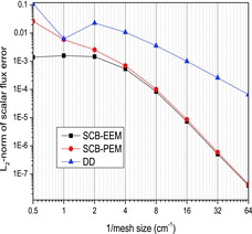
The order of convergence of new methods is numerically analyzed for a one-group homogeneous problem as for mesh refinements. The first test problem is a 2.0-cm thick homogeneous slab with vacuum condition at both boundaries. The macroscopic total and scattering cross sections are 2.0 and 1.0 cm⁻¹, respectively. The source of 1.0 #/cm³ sec is uniformly distributed in the slab. For this problem, we considered eight mesh sizes of 2.0, 1.0, 1/2, 1/4, 1/8, 1/16, 1/32, and 1/64 cm to show the convergence of the methods as the mesh size decreases. S₁₂ angular quadrature was used and the results of the diamond differencing (DD) are compared with those of new methods. The exact solutions of the discrete ordinates transport equation with S₁₂ angular quadrature are obtained using the eigenfunction expansion and the vacuum boundary conditions. Then, the L₂-norm of the errors for each mesh size were evaluated using (47) $$E_I=\sqrt{\frac{1}{I}\sum _{i=1}^I{({\phi }_{\mathrm{nume},i}-{\phi }_{\mathrm{exact},i})}^2},$$(47) where φ_{nume, i} and φ_{exact, i} are the numerically estimated and exact scalar fluxes for the mesh i, respectively, and I is the total number of meshes. Figure 2 compares the variations of the L₂ norm of the errors for new methods and DD versus the inverse of the mesh size. This figure shows that DD has its well-known second-order behavior of the convergence while the new eigenfunction and polynomial expansion methods with sub-cell balances have third-order convergence as the mesh size decreases. It is also noted that SCB-EEM gives much smaller values of the L₂ norm of errors for large mesh sizes than SCB-PEM and DD.

Figure 2. Comparison of the L₂-norms of errors versus mesh size.

3.2. Numerical tests for multi-group problems

In this subsection, the new methods were tested for multi-group test problems. First, new methods are applied to a two-group heterogeneous problem consisting of four regions. The configuration and sources are given in Figure 3. The cross sections are given in Table 1.

Table 1. Cross sections (cm⁻¹) for the two-group heterogeneous problem.

			Scattering cross
			sections
	Energy	Total cross
Regions	group (g)	sections	1 → g	2 → g
I	1	0.3	^a0.27	^a0.001
			^b0.09	^b0.0002
	2	1.0	0.01	0.90
			0.002	0.08
II	1	0.2	0.18	0.001
			0.08	0.0003
	2	3.53	0.01	0.53
			0.003	0.06
III, IV	1	0.401	0.32	0.002
			0.07	0.0004
	2	1.30	0.08	1.29
			0.003	0.20

^aIsotropic component.

^bLinearly anisotropic component.

Figure 3. Configuration and sources of the two-group heterogeneous test problem.

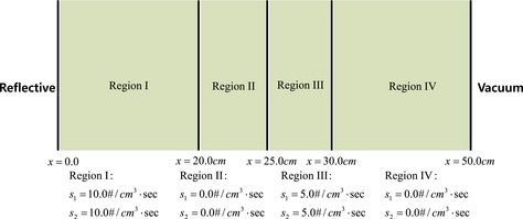
The left and right boundary conditions are reflective and vacuum, respectively. The sources are given in regions I and III. Region II has large absorption cross section for the second energy group and no source, and so the scalar flux will be very small in this region. The thicknesses of regions I, II, III, and IV are 20, 5, 5, and 20 cm, respectively. For this test problem, four different mesh divisions were used to show the effect of the mesh sizes on the accuracy. This problem is solved with S₁₂ angular quadrature.

Table 2 summarizes the results of numerical analyses with three different mesh division types. In this numerical test, the region average scalar fluxes and the scalar flux at the right boundary are analyzed as the function of the mesh division types and the reference solution was obtained using DD with very fine meshes such that each region was divided into 1000 meshes. These results show that SCB-EEM1 gives quite accurate solutions even with large mesh size for both energy groups. For example, SCB-EEM1 even with 2, 1, 1, and 2 meshes in region I, II, III, and IV, respectively, gives extremely small errors less than 0.2% for all the region average scalar fluxes, 2.6% (Group 1) and 4.2% (Group 2) errors of the scalar fluxes at the right boundary. SCB-EEM2 also gives much higher accuracy for most of the mesh sizes than DD and its solution converges to that of SCB-EEM1 as mesh size decreases. SCB-PEM shows much higher accuracies for thick meshes than DD.

Table 2. Relative errors (%) of the region average scalar fluxes and the scalar fluxes at the right boundary.

	DD		SCB-EEM1		SCB-EEM2		SCB-PEM
Region no.	Group 1	Group 2	Group 1	Group 2	Group 1	Group 2	Group 1	Group 2
I	^a0.25	0.38	0.01	0.00	−0.02	0.10	0.23	4.50
	^b0.02	0.09	0.00	0.01	0.00	0.01	0.02	0.50
	^c0.0	−0.06	0.00	0.01	0.00	0.01	0.00	0.03
II	3.94	1096.2	−0.20	0.08	−0.15	0.55	0.35	−29.8
	0.26	242.9	−0.03	−0.01	−0.03	0.00	0.06	−3.46
	0.03	−0.03	0.00	−0.08	0.00	−0.08	0.01	−0.20
III	2.81	−14.79	0.07	−0.03	0.10	0.43	2.34	39.2
	0.13	−0.10	0.02	−0.02	0.02	0.01	0.27	4.98
	0.01	0.31	0.01	0.09	0.01	0.09	0.01	0.27
IV	27.3	38.94	−0.13	−0.187	−0.47	−1.80	3.43	16.94
	0.03	1.07	−0.04	−0.02	−0.05	−0.08	0.54	2.10
	0.1	0.55	0.01	0.03	0.01	0.03	0.03	0.11
At right boundary	123.4	389.9	−2.62	−4.18	−13.49	−18.56	15.35	2.02
	−3.06	−11.2	−0.83	−3.14	−0.94	−3.36	0.23	−3.19
	0.64	0.17	0.01	−0.60	0.01	−0.61	0.06	−0.64

^a2,1,1 and 2 meshes are used in regions I, II, III, and IV, respectively.

^b8,4,4, and 8 meshes are used in regions I, II, III, and IV, respectively.

^c32,16,16, and 32 meshes are used in regions I, II, III, and IV, respectively.

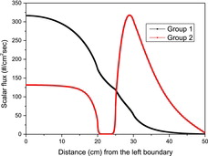
The scalar flux distributions that are obtained with the reference fine mesh DD calculation are shown in Figure 4. As expected, there are very steep gradients of the second-group scalar flux near the interfaces of region II.

Figure 4. Reference scalar flux distribution for the two-group heterogeneous test problem.

The next test problem is a 40-cm thick homogeneous slab with four group cross sections. This problem consists of source region and shield region while they have the same cross sections. The configuration of this problem and source strengths are given in Figure 5 and the four group cross sections are provided in Table 3. The boundary conditions at the left and right boundaries are reflective and vacuum, respectively. The shield region is sub-divided into three regions of equal thickness for comparison of the region average scalar fluxes.

Table 3. Multi-group cross sections (cm⁻¹) for the four-group homogeneous test problem.

		Scattering cross sections
Energy group (g)	Total cross section	1 → g	2 → g	3 → g	4 → g
1	0.5	3.000E−01	5.000E−02	1.000E−04	4.000E−04^a
		2.900E−02	3.500E−04	2.500E−05	2.100E−05^b
2	1.0	1.000E−02	5.000E−01	5.000E−03	1.000E−03
		1.500E−04	1.200E−02	1.800E−04	4.100E−05
3	2.0	5.000E−03	2.000E−01	1.000E+00	8.000E−02
		2.400E−04	2.950E−03	5.000E−02	1.800E−04
4	4.5	1.000E−03	1.000E−01	8.000E−02	2.000E+00
		3.700E−05	2.600E−02	4.500E−04	6.800E−02

^aIsotropic component.

^bLinearly anisotropic component.

Figure 5. Configuration and sources of the four-group test problem.

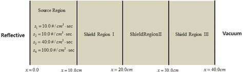
The S₁₂ angular quadrature was used for this test problem. The accuracy of the region average scalar fluxes and the scalar fluxes at the right boundary was analyzed in comparison of the reference solution obtained with a very fine mesh DD calculation (mesh size = 0.01 cm). The analysis results are given in Table 4. All the methods give quite accurate values of the source region average first-group scalar flux for all the mesh sizes. For the other region average scalar fluxes and the one at the right boundary, all the new methods except for DD give quite accurate values whose errors are less than 1% for all the mesh sizes with one exception for the largest mesh size case of 5.0 cm.

Table 4. Relative errors (%) of the region average fluxes and scalar fluxes at the right boundary for the four-group homogeneous test problem.

		Method
Region	Mesh size (cm)	DD	SCB-EEM1	SCB-EEM2	SCB-PEM
Source region	5.0	^a0.6/^b0.6/^c0.5	0.1/0.0/0.0	0.0/0.0/0.0	0.3/0.7/0.6
	2.5	0.2/0.2/0.2	0.0/0.0/0.0	0.0/0.0/0.0	0.1/0.2/0.4
	1.25	0.0/0.1/0.1	0.0/0.0/0.0	0.0/0.0/0.0	0.0/0.0/0.2
	0.625	0.0/0.0/0.0	0.0/0.0/0.0	0.0/0.0/0.0	0.0/0.0/0.1
	0.3125	0.0/0.0/0.0	0.0/0.0/0.0	0.0/0.0/0.0	0.0/0.0/0.0
Shield region I	5.0	48.4/183.2/547.5	−0.6/−0.5/−0.7	−0.1/0.1/3.3	−3.7/−16.2/−62.7
	2.5	11.4/61.4/505.1	−0.4/−0.6/−0.3	−0.3/−0.4/1.4	−0.9/−4.6/−41.0
	1.25	0.6/12.7/257.5	−0.1/−0.5/−0.2	−0.1/−0.5/−0.3	−0.2/−1.2/−19.0
	0.625	0.1/1.7/84.7	0.0/−0.2/−0.5	0.0/−0.2/−0.5	0.0/−0.3/−6.0
	0.3125	0.0/0.0/18.2	0.0/0.0/−0.6	0.0/0.0/−0.6	0.0/0.0/−1.6
Shield region II	5.0	−12.5/48.4/90.4	0.0/1.7/2.9	−0.9/−20.6/−10.4	8.8/129.6/1747.3
	2.5	−22.3/−1.8/41.2	0.0/0.0/0.0	0.1/−1.3/−7.7	0.3/1.1/16.3
	1.25	−11.0/−10.5/−0.2	0.0/0.0/0.0	0.0/−0.1/−0.9	0.0/0.0/0.0
	0.625	−2.9/−3.6/−2.0	0.0/0.0/0.0	0.0/0.0/−0.1	0.0/0.0/0.0
	0.3125	−0.7/−0.9/−0.9	0.0/0.0/0.0	0.0/0.0/0.0	0.0/0.0/0.0
Shield region III	5.0	30.3/142.0/209.3	0.7/0.8/0.9	−0.3/−20.0/−16.6	14.7/57.1/1924.2
	2.5	−47.8/−29.9/16.6	0.0/0.0/0.1	0.0/−1.2/−6.6	0.6/0.0/0.8
	1.25	−20.7/−18.4/−9.8	0.0/0.0/0.0	0.0/0.1/−0.8	0.0/0.0/0.0
	0.625	−5.5/−5.5/−4.3	0.0/0.0/0.0	0.0/0.0/0.1	0.0/0.0/0.0
	0.3125	−1.4/−1.4/−1.4	0.0/0.0/0.0	0.0/0.0/0.0	0.0/0.0/0.0
Right boundary	5.0	91.3/444.6/879.5	−0.3/−3.1/−8.2	−1.3/82.8/354.8	29.5/586.1/98302.6
	2.5	−64.1/−34.5/140.0	−0.8/−3.4/−7.8	−0.9/−8.4/67.6	−0.2/−5.2/−27.9
	1.25	−29.5/−11.7/55.3	−0.3/−1.8/−5.9	−0.3/−2.1/−22.9	−0.3/−2.4/−17.0
	0.625	−8.2/−8.2/23.3	0.0/−0.5/−4.5	0.0/−0.5/−5.5	0.0/−0.6/−8.9
	0.3125	−2.1/−2.1/−2.1	0.0/0.1/−2.7	0.0/−0.1/−2.6	0.0/−0.1/−3.9

^aGroup 1.

^bGroup 2.

^cGroup 4.

The errors of Group 2 are relatively larger than those of Group 1 due to the shorter mean free path of Group 2 neutrons. However, the new methods using eigenfunction expansion still give quite accurate region average scalar fluxes. For SCB-EEM1, the errors for all the regions are less than 1% for all the mesh sizes with one exception for the shield region II with mesh size of 5.0 cm. Also, SCB-EEM2 gives quite accurate results whose errors are less than 1.3% for all the regions and mesh sizes with one exception for 5.0-cm mesh size. SCB-PEM also gives much higher accuracy than DD but their solutions are less accurate than the eigenfunction expansion methods. It is noted that the accuracy of SCB-PEM is comparable to the eigenfunction expansion methods except for the shield region I and the other shield regions in the 5.0-cm mesh size cases. Our methods also give quite accurate values of the scalar flux at the right boundary. In particular, SCB-EEM1 gives errors less than 3.5% for all the mesh sizes.

The accuracies of all the methods for Group 3 are worse than those for Group 2, but the trends versus mesh size variations are similar to each other. For this reason, the results for Group 3 are omitted. As shown in the table, the errors for Group 4 are larger than those for the previous energy groups. It is due to the fact that this energy group has the shortest mean free path (i.e., largest total cross section) and large ratio of absorption-to-total cross section. However, Table 4 shows that SCB-EEM1 still gives extremely accurate results for the region average scalar fluxes for all the meshes. The errors of SCB-EEM1 are less than 1% for all the cases with one exception for the shield region II with 5.0-cm mesh size. On the other hand, the scalar fluxes at the right boundary are relatively small in comparison with the region average scalar fluxes (see Figure 6) and so it is quite difficult for the scalar flux at the right boundary to be accurately estimated although it is a homogeneous problem. For SCB-EEM1, the errors of the scalar flux at the right boundary are 8.2% and 2.7% for 5.0 and 0.31-cm mesh sizes, respectively. SCB-EEM2 also shows larger errors than in the previous energy groups but its errors for the shield region II are much smaller than those of DD and SCB-PEM while SCB-PEM shows comparable accuracies for the shield region III and the right boundary to SCB-EEM2 except for the case of 5.0-cm mesh size in which the errors of Groups 2 and 4 scalar fluxes are unphysically large for DD, SCB-EEM2, and SCB-PEM.

Figure 6. Reference scalar flux distributions for the four-group test problem.

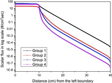
Figure 6 shows the scalar flux distributions in log-scale which are obtained by the very fine mesh DD calculation. As expected, it is noted in this figure that the last-group scalar flux is rapidly reduced at the right boundary and it has very steep gradient near the interface between the source and shield regions.

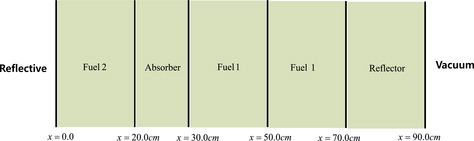
The last test problem is a two-group eigenvalue problem that consists of five material regions (three fuel regions, one absorber region, and one reflective region). As shown in Figure 7, each region is a 20-cm thick slab except for the absorber region of 10 cm. An absorber region having large thermal absorption cross section is placed between two fuel regions. The two-group cross sections for these regions that are given in Table 5 are from the small LWR problem given in [18]. Fuel 2 is devised to model fuel region having lower enriched uranium than Fuel 1. Fuel 2 has the same cross sections as Fuel 1 except for its thermal nu*fission cross section. S₁₂ quadrature set is used to solve this problem.

Table 5. Cross sections (cm⁻¹) for the two-group eigenvalue problem.

				Scattering
Materials	Energy group (g)	Total	Nu*fission	1 → g	2 → g
Fuel 1	1	2.23775E−01	9.09319E−03	1.92423E−01	0.00000E+00
	2	1.03864E+00	2.90183E−01	2.28253E−02	8.80439E−01
Fuel 2	1	2.23775E−01	9.09319E−03	1.92423E − 01	0.00000E+00
	2	1.03864E+00	2.00000E−01	2.28253E − 02	8.80439E − 01
Reflector	1	2.50367E−01	0.00000E+00	1.93446E−01	0.00000E+00
	2	1.64482E + 00	0.00000E + 00	5.65042E − 02	1.62452E+000
Absorber	1	8.52325E − 02	0.00000E + 00	6.77241E − 02	0.00000E+00
	2	2.17460E−01	0.00000E+00	6.45461E−05	3.52358E−02

Figure 7. Configuration of the two-group eigenvalue problem.

The eigenvalues estimated with the new methods versus the number of meshes per region are given in Table 6. The results show that SCB-EEM1 gives quite accurate values even with only one mesh per region (i.e., 20-cm mesh size) and SCB-PEM gives greater accuracies for eigenvalues than SCB-EEM2. DD gives less accurate results in eigenvalue for the cases using one and two meshes per each region than our methods while it gives accurate eigenvalues comparable to those of our methods for the cases having six and four meshes per region. The reference eigenvalue and flux distribution are obtained using DD and 400 meshes for each region.

Table 6. Comparison of the eigenvalues for the eigenvalue problem.

Numbers of meshes per region	SCB-EEM1	SCB-EEM2	SCB-PEM	DD
1	1.405239 (−0.14^a)	1.440578 (2.37)	1.402820 (−0.31)	3.6604 (160)
2	1.407416 (0.02)	1.417884 (0.76)	1.405594 (−0.11)	1.42097 (0.98)
4	1.407295 (0.01)	1.409521 (0.17)	1.406993 (−0.01)	1.40725 (0.01)
6	1.407224 (0.00)	1.407958 (0.06)	1.407149 (0.00)	1.406329 (-0.06)
Reference	1.407164

^a(k_eff − k_{eff,reference})/k_{eff,reference} × 100.

The region average scalar fluxes are compared in Table 7. The results show that SCB-EEM1 gives very accurate values even with one mesh per each region and maximum relative error for Group 1 is 4.85% in the reflector region. SCB-EEM2 shows reasonable accuracy except for the one mesh case per region while SCB-PEM gives similar accuracies to SCB-EEM2 except for the reflector region.

Table 7. Comparison of the relative percentage errors of the region-wise scalar fluxes.

		Method
Region	Number of meshes per region	SCB-EEM1	SCB-EEM2	SCB-PEM	DD
Region I (fuel 2)	1	^a2.23/^b2.41	−12.51/−15.10	10.13/12.97	−93.1/92.8
	2	0.28/0.33	−4.71/−5.37	3.94/5.06	−9.5/−8.5
	4	0.07/0.10	−1.10/−1.18	0.95/1.27	0.1/0.1
Region II (absorber)	1	−0.82/−0.47	−4.17/−59.2	8.07/−28.3	−91.7/112.9
	2	−0.34/−0.54	−2.21/−17.8	3.26/−12.3	−10.6/58.6
	4	−0.06/−0.37	−0.64/−3.29	0.80/−3.74	0.0/6.5
Region III (Fuel 1)	1	0.94/0.91	−3.72/−1.05	3.15/4.36	−64.8/−72.2
	2	0.04/0.05	−1.57/−0.90	1.18/1.51	−6.5/−3.8
	4	−0.01/0.00	−0.41/−0.30	0.23/0.32	−0.8/−0.6
Region IV (fuel 1)	1	−1.99/−0.95	1.16/3.90	−1.57/−6.06	−44.8/97.2
	2	−0.19/−0.07	0.65/1.83	−0.66/−2.19	4.5/5.0
	4	0.00/−0.02	0.20/0.49	−0.15/−0.49	0.4/0.6
Region V (reflector)	1	−4.85/1.29	−1.22/15.42	−18.64/1.20	107.8/55.7
	2	0.37/−0.06	0.81/−3.32	−6.15/−0.20	53.7/125.6
	4	−0.09/−0.09	0.32/−0.95	−1.45/−0.15	7.7/15.9

^aGroup 1.

^bGroup 2.

For Group 2, SCB-EEM1 still shows very accurate region average fluxes even with one mesh per each region and maximum error is 2.41%. SCB-EEM2 and SCB-PEM give much larger errors in the absorber region for the cases using small number of meshes. DD gives much larger errors in the region average scalar fluxes than our methods and it is noted that DD gives large errors in the reflector region even for the case using four meshes per region.

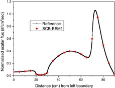
Figures 8 and 9 compare the scalar flux distributions obtained by the reference DD calculation and SCB-EEM1 using four meshes per each region for Groups 1 and 2, respectively. These figures show that SCB-EEM1 gives accurate scalar flux distributions with large mesh size.

Figure 8. Comparison of the scalar flux distributions for the two-group eigenvalue problem (Group 1).

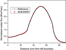
Figure 9. Comparison of the scalar flux distributions for the two-group eigenvalue problem (Group 2).

4. Conclusion

In this paper, a new accurate solution method using eigenfunction expansion and sub-cell balances was developed for solving the multi-group even-parity discrete ordinates transport problem with a linearly anisotropic scattering source in slab geometry and it was tested for one- and multi-group problems including an eigenvalue problem as well as fixed source problems. The four eigenfunctions of S₄ within-group transport equation are used as basis functions to expand the spatial shape of angular flux in each mesh. The cubic and constant shape approximations were introduced for the spatial shape of the scattering source from other energy groups and fission source. In the new methods, the coupling equations for the unknowns were derived using the two sub-cell balance equations and two continuity conditions of the odd- and even-parity angular fluxes at both edges. For the accuracy analysis of new methods, a sub-cell method with polynomial expansion of angular flux was also developed.

The new methods were applied to various test problems for performances analysis. The results of one-group homogeneous problem showed that the new methods are third-order accurate in mesh refinements. The tests for multi-group problems also showed that new methods give accurate region average scalar fluxes and the boundary scalar fluxes. In particular, the sub-cell balance method with eigenfunction expansion and with cubic spatial approximation of the sources gave quite accurate scalar fluxes and eigenvalues even with very thick meshes for both multi-group fixed source and eigenvalue problems. From the numerical tests, it can be concluded that the newly developed eigenfunction expansion methods with sub-cell balances can be effectively used in the multi-group slab geometry problems for accurate estimation of the scalar flux distributions and eigenvalues.

The novelty of the newly developed method in this paper resides in the use of the eigenfunctions of the S₄ approximation to represent the within-group, even-parity angular flux and a cubic polynomial to approximate the scattering sources from other energy groups and the fission source. The idea was proposed in one of the authors’ earlier work: the idea for one-group, slab-geometry problems with isotropic scattering was introduced in [11] and extended it for linearly anisotropic scattering in [12]. This paper successfully extended the idea for multi-group problems.

Additional information

Funding

This work was supported by a grant from the Kyung Hee University in 2012 [grant number KHU-20121703].

References

- Lewis EE, Miller WF. Computational methods of neutron transport. New York (NY): John Wiley; 1984.
- Duderstadt JJ, Martin WR. Transport theory. New York (NY): John Wiley; 1979.
- Carlson BG, Lathrop KD. Transport theory– the method of discrete ordinates, computing methods in reactor physics. In: Greenspan H., Kelber CN, and Okrent D, editors. New York (NY): Gordon and Breach; 1968.
- Sanchez R, McCormick NJ. A review of neutron transport approximation. Nucl Sci Eng. 1982;80:481–535.
- Lathrop KD. Spatial differencing of the transport equation: positivity vs. accuracy. J Comput Phys. 1969;4:475–498.
- Barros RC, Larsen EW. A numerical method for one-group slab-geometry discrete ordinates problems with no spatial truncation error. Nucl Sci Eng. 1990;104:199–208.
- Hong SG, Cho NZ. The infinite medium Green's function method for multigroup discrete ordinates transport problems in multi-layered slab geometry. Ann Nucl Energy. 2001;28:1101–1114.
- Barichello LB, Garcia RDM, Siewert CE. Particular solutions for the discrete-ordinates method. J Quant Spectrosc Radiat Transf. 2000;64:219–226.
- Vilhena MT, Barichello LB. An analytic solution for the multigroup slab geometry discrete ordinates problem. Transp Theory Stat Phys. 1995;24:1337–1352.
- Noh JM, Cho NZ. A new approach of analytic basis function expansion to neutron diffusion nodal calculation. Nucl Sci Eng. 1994;116:165–180.
- Hong SG, Kim SJ, Kim YJ, Kim YI. High-order function expansion nodal methods for the even-parity transport equation in slab geometry. Trans Am Nucl Soc. 2002;86:215.
- Hong SG, Kim SJ, Kim YJ, Kim YI. The eigenfunction expansion nodal methods for the even-parity transport equation with anisotropic scattering. Paper presented at: International Conference on the New Frontiers of Nuclear Technology: Reactor Physics, Safety, and High-Performance Computing (PHYSOR2002); 2002 October 7–10; Seoul, Korea.
- Morel JE, Larsen EW. A multiple balance approach for differencing the Sn equations. Nucl Sci Eng. 1990;105:1–15.
- Adams ML. Subcell balance methods for radiative transfer on arbitrary grids. Transp Theory Stat Phys. 1997;26:385–431.
- Park CJ, Cho NZ. A linear multiple balance method with high-order accuracy for discrete ordinates neutron transport equations. Ann Nucl Energy. 2001;28:1499–1517.
- Hong SG. Two subcell balance methods for solving the multigroup discrete ordinates transport equation with tetrahedral meshes. Nucl Sci Eng. 2013;173:101–117.
- Cho NZ, Noh JM. Hybrid of AFEN and PEN methods for multigroup diffusion nodal calculation. Trans Am Nucl Soc. 1995;73:438–440.
- Takeda T, Ikeda H. 3-D neutron transport benchamrks. J Nucl Sci Technol. 1991;28:656–669.