Seismic response analysis of full-scale boiling water reactor using three-dimensional finite element method

Abstract

This paper presents the three-dimensional finite element seismic response analysis of full-scale boiling water reactor BWR5 at Kashiwazaki-Kariwa Nuclear Power Station subjected to the Niigata-ken Chuetsu-Oki earthquake that occurred on 16 July 2007. During the earthquake, the automatic shutdown system of the reactors was activated successfully. Although the monitored seismic acceleration significantly exceeded the design level, it was found that there were no significant damages of the reactor cores or other important systems, structures and components through in-depth investigation. In the seismic design commonly used in Japan, a lumped mass model is employed to evaluate the seismic response of structures and components. Although the lumped mass model has worked well so far for a seismic proof design, it is still needed to develop more precise methods for the visual understanding of response behaviors. In the present study, we propose the three-dimensional finite element seismic response analysis of the full-scale and precise BWR model in order to directly visualize its dynamic behaviors. Through the comparison between both analysis results, we discuss the characteristics of both models. The stress values were also found to be generally under the design value.

Keywords:

• finite element method
• nuclear reactor
• numerical simulation
• three-dimensional FE seismic response analysis
• parallel calculation
• BWR
• Kashiwazaki-Kariwa nuclear power plant
• lumped mass model
• seismic design

1. Introduction

Seismic design for nuclear power plants (NPP) is extremely important to construct and operate in earthquake-prone countries such as Japan. What reminded us of its importance was the Niigata-ken Chuetsu-Oki earthquake occurred on 16 July 2007, with a magnitude of 6.8. Due to this earthquake, a seismic vibration with intensity 7 was measured at Kashiwazaki-Kariwa Nuclear Power Station owned by Tokyo Electric Power Company (TEPCO), and was located approximately 16 km apart from the epicenter of the earthquake, and there were some damages in the plant. When the earthquake occurred, three reactors, Unit 3, 4 and 7, had been under operation at their rated power. The observed maximum response acceleration exceeded the response acceleration that was estimated from the design basis earthquake, and the observed response spectrums largely exceeded the response spectrums that were estimated from the design basis earthquake over all the frequency range. Although no significant damages were found in the equipment important to safety [1,2], the plant has been shut down for a significant period of time for the safety inspection and the earthquake countermeasures.

The authors conducted three-dimensional (3D) analyses of boiling water reactor (BWR) and advanced boiling water reactor (ABWR) in the Kashiwazaki-Kariwa Nuclear Power Station using the finite element (FE) method, in order to evaluate precisely their seismic response behaviors. Observed seismic wave and design basis earthquake were assumed for the excitation condition. We performed the analyses from 2008 to 2010, and presented the results in the Atomic Energy Society of Japan (AESJ) and other conferences [3–7]. In the middle of compiling a paper, on 11 March 2011, the earthquake off the Pacific coast of Tōhoku struck offshore of Japan and the earthquake triggered huge tsunami waves. In all the 11 plants in operation, the control rods were inserted and automatically shut down out of the 14 ones (total electric power: 12,370 MW) of the four nuclear power plants that are located on the region (TEPCO's Fukushima Daiichi and Fukushima Daini Nuclear Power Stations, Tohoku Electric Power Company's Onagawa Nuclear Power Station and the Japan Atomic Power Company's Tōkai Daini Nuclear Power Station). The eight plants have shut down successfully in cold condition and were kept stable; however, Units 1–4 out of the six units of TEPCO's Fukushima Daiichi Nuclear Power Station resulted in serious accidents due to the loss of cooling function for nuclear reactors or storage pools for the spent nuclear fuels. For this accident, strenuous efforts have continued even until now. The authors would like to express our condolences for people who suffered from the earthquake and the accident of the NPPs.

The authors have suspended working on our paper on the analysis of the Kashiwazaki-Kariwa Nuclear Power Station, since the 3.11 earthquake. However, the analysis method we conducted will be valid for understanding the state of the reactors that are exposed to the seismic force exceeding the design seismic motion, and no similar analysis with models that are as precise as ours has been found. The authors started again writing our paper with a view of enhancing the seismic analysis technique of a nuclear power reactor or an NPP.

TEPCO's Kashiwazaki-Kariwa Nuclear Power Station was the largest NPP in the world which has seven reactors including five BWRs of Units 1–5 and two ABWRs of Units 6 and 7. When the Niigata-ken Chuetsu-Oki earthquake occurred, Units 3–5 were under operation at their rated power, Unit 2 was under a start-up operation after periodic inspection, and Units 1, 5 and 6 were not operating under periodic inspection. Units 2, 3, 4 and 7 were shut down safely by a reactor shutdown system in response to the earthquake. TEPCO and Nuclear and Industrial Safety Agency (NISA) conducted a series of seismic analyses using a lumped mass model (LMM) and plant walkdowns. The team confirmed that the plant was shut down safely as intended and that the core cooling and radiation shield were successfully operated. International Atomic Energy Agency (IAEA) also conducted their own investigation, and recognized the results of the TEPCO and NISA team to be appropriate. In this paper, the reactor that the authors analyze is Unit 5 that has the same design called BWR5 as Units 1–4. The monitored seismic acceleration has been used for the excitation condition.

In the seismic design for NPP in Japan, seismic analyses are conducted using the LMM, accelerations or stresses are calculated and then each equipment is evaluated using these values. Although the LMM seems simple, empirical or experimental experiences over many years are reflected to parameter values such as mass densities, spring constants or damping factors in the model, and the model has sufficient capability in evaluating seismic response of the system. However, it needs some expertise to grasp analysis results intuitively because the LMM does not represent geometries of components. In evaluating each component by the LMM, since the geometry is modeled by a beam model in most settings, the results may include large safety margin. The authors conducted a seismic analysis by 3D FE analysis of a reactor pressure vessel (RPV) including core internals, with a detailed FE mesh model on a parallel computer. By using the results of the analysis, visualizing the seismic behavior of the components in a comprehensible way, the authors compared the results with the LMM and went through characteristics and problems of the FE analysis.

Our analysis object is the RPV and the core internals. As will be stated in the following sections, the geometry of each component has been modeled with solid elements except for connection joints and constraint sections. The authors confirmed that the overall behavior of the RPV, the fuel assemblies or the control rod drive (CRD) housing agreed well with those of the LMM analysis. On this basis, we could observe some behaviors that only the 3D analysis can reproduce. The present FE analysis refers to the seismic design standard and the LMM analysis based on the standard in the process of modeling and analysis.

As will be shown in the following sections, the FE model is highly complicated and large. For this reason, the authors used the analysis code ADVENTURECluster (ADVC) [8], which was developed with the aim of large-scale analysis based on the parallel processing. ADVC is built based on ADVENTURE system, which was developed by ADVENTURE project [9]. On this basis, ADVC has wide range of functions as general purpose structural analysis code, and has a number of users in automobile, electronics, energy, precision equipment industries and others.

Although the detailed 3D FE model has been constructed, the authors simplified or neglected some components, based on the judgment that there would be no significant effect on the analysis results. Although reactor water affects the motion of the reactor core, we considered the reactor water just as an added mass, because ADVC has no corresponding function, whereas Kataoka et al. [10] has been working on acoustic fluid-structural coupling analysis.

This work is the first attempt in the world which visualizes the 3D seismic behavior of the nuclear reactor and conducts more detailed evaluation [3–7]. The authors expect that the FE analysis becomes a major evaluation tool for seismic analysis and eventually for various accident assessments of NPPs.

2. Overview of the analysis code

3D FE analysis code ADVC has a linear solver named CGCG (coarse grid conjugate gradient) method [11] that assumes large-scale analysis based on a domain decomposition method. The CGCG method is summarized as follows. In a static analysis, let the stiffness equation be (1) $$Ku=f$$(1) where u is the displacement vector, K is the stiffness matrix and f is the external force vector. In the nonlinear analysis or the dynamic response analysis, the latter of which is our analysis in the present study, the equation has the following incremental form: (2) $$K\Delta u=\Delta f$$(2) which is the same form of Equation (1). In this case, K is called the tangent stiffness matrix.

In a large-scale analysis, Equation (1) or Equation (2), the degrees of freedom (DOFs) are assumed to be large. In the CGCG method, an analysis object domain Ω is divided into an FE mesh model, and the mesh model is decomposed into an appropriate number of subdomains. A part of those subdomains is used for the parallel processing and evaluation of the motion of the subdomains themselves. The motion of the subdomains is incorporated into a process of solving Equation (1) or Equation (2). Let V be the space of the admissible displacement of Equation (1) or Equation (2). V is decomposed into two subspaces W₁ and V₁ as follows: (3) $$V=W_1{\oplus }_K{V}_1$$(3) where W₁ is the space of the global coarse motion of the subdomains (e.g. the rigid body motion of the subdomains) and V₁ is the conjugate orthogonal space of W₁ with respect to K.

If needed, a subspace W₂ of V₁ is taken, which is another coarse space that does not include the motion in W₁: (4) $$V_1=W_2{\oplus }_K{V}_2$$(4)

V is given as follows: (5) $$V=W_1{\oplus }_K{W}_2{\oplus }_K{V}_2$$(5)

This procedure is continued, applying the direct method to W₁, W₂, …, and the iterative method (CG method) is applied to the last conjugate space.

In this paper, the linear time-dependent response equation (6) $$M\ddot{u}+C\dot{u}+Ku=f\left(t\right)$$(6) is assumed, where u is the displacement vector, M is the mass matrix, C is the damping matrix, K is the stiffness matrix and f is the time-dependent external force vector. The incremental displacement Δu is assumed to be the time-dependent unknown vector, and Equation (2) as an incremental form of stiffness equation is derived. In the FE analysis, the damping effect is assumed to be the so-called Rayleigh damping in general [12]. The damping matrix C is assumed in the following form: (7) $$C=\alpha M+\beta K$$(7)

In comparison with the LMM, α and β are determined by a damping factor of each component given as the design basis and eigenvalues of each component obtained from the FE analysis. Determination of C will be stated in Section 3.6.

Parallel performance of ADVC is high. Some of the present authors conducted analyses such as a drop impact analysis of a cell phone with 305 million DOFs with 8124 parallel processes [13] and a nonlinear seismic response analysis of a high-rise office building with 75 million DOFs with 1024 parallel processes [14].

3. Construction of 3D FE model of BWR RPV and core internals

In our study, the analysis object is the BWR5-type RPV and the core internals of TEPCO Kashiwazaki-Kariwa Nuclear Power Station. Construction of the FE analysis model starts from computer aided design (CAD) model, then a mesh model is generated and finally various analysis conditions are assigned. This procedure is described in this section (see also [3–7]).

As briefly noted in Section 1, there exist restrictions and prior requirements:

1. The reactor water is not modeled, but considered as the added mass instead.

2. Neglect constraints by piping systems as those effects are restricted to the seismic behavior of the RPV.

3. When a component is highly complicated, assume simplification corresponding to its physical characteristics.

4. Let the LMM be the analysis standard, take the material properties in the LMM analysis.

5. Take the LMM results as the reference standard as well.

Note that in the LMM, the reactor water is considered as the added mass to each component (e.g. core shroud and RPV) and as the mutual added mass between components, and those terms are included in the mass matrix.

3.1. CAD model

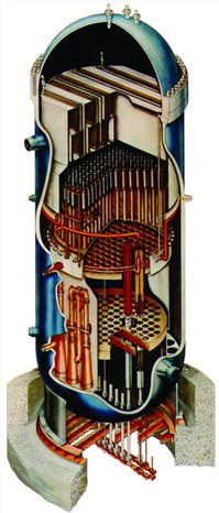
Generally, in the design process, 3D CAD models are used for interference check for the components. Figure 1 shows an original CAD model of a nuclear reactor. Our study starts from this CAD model.

Figure 1. CAD model of BWR.

3.2. LMM

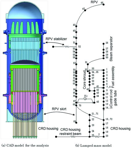
In the seismic design of NPPs, the LMM is used to determine seismic loads that are applied to structural design of each component. From the viewpoint of various past results, our FE analysis refers to data settings or analysis results as the reference standard. Figure 2(b) shows the LMM model of our analysis in comparison with the CAD model for our analysis shown in Figure 2(a).

Figure 2. CAD model for analysis and lumped mass model.

3.3. Simplification of the CAD model

Although large-scale analysis is available, it is not realistic to construct the entire detailed model represented in the original CAD model. Some parts of the CAD model for the FE analysis have been simplified or neglected in the following way. First, small size pipes, studs, small size brackets or measuring equipment housings have been neglected as they have not affected the seismic behavior significantly. If the mass of the components cannot be neglected, it has been considered as the added mass to other components. Since the fuel assemblies have especially complicated shape, the shape has been simplified, and the stiffness and the mass have been taken to be equivalent to the actual fuel assemblies. Similarly, the only geometry of the steam dryer that has complicated shape has been modeled, and the mass has been taken to be equivalent to the design. The control rod drive mechanism (CRDM) housings or the stand pipes of the steam dryer that have the shape of thin-walled cylinder have been simplified as solid cylindrical bodies. As mentioned above, the geometries of the CRDM, the steam dryer and the steam–water separator have been simplified. However, the first eigenmodes of the FE analyses of the respective components are taken to be identical with the respective LMM results as far as possible. Also, note that the only RPV mesh was generated from the CAD model. Table 1 shows the components of the CAD model used for the analysis and the number of pieces and materials.

Table 1. CAD model for the analysis.

Components	No.	Material
Reactor vessel (RPV) body	1	Low-alloy steal
Reactor vessel (RPV) cover	1	Low-alloy steal
Reactor vessel skirt	1	Low-alloy steal
Shroud support	1	Inconel alloy
Shroud support plate	1	Inconel alloy
Shroud support leg	12	Inconel alloy
Core shroud	1	SUS
Control rod drive housing stab tube	185	Inconel alloy
Core support plate	1	SUS
Control rod drive	185	SUS
Control rod drive housing	185	SUS
Control rod guide tube	185	SUS
Fuel assembly support	185	SUS
Fuel assembly	740	Composite body
Around fuel assembly support	24	SUS
Around fuel assembly	24	SUS
Circumferential plate of upper grid plate	1	SUS
Grid of upper grid plate	1	SUS
Steam separator stand pipe	225	SUS
Steam separator securing bracket	40	SUS
Steam separator securing ring	2	SUS
Shroud head	1	SUS
Steam dryer	1	SUS
Steam dryer top panel	1	SUS
Steam dryer skirt	1	SUS
Jet pump head, riser tube and riser tube support	10	SUS
Jet pump inlet mixer and diffuser	20	SUS
Jet pump weld overlay and bracket	20	SUS

3.4. Component mesh and connection of the components

As to the global coordinate system, the x-axis is taken to be from south to north (S–N), the y-axis from west to east (W–E) and z-axis from upward vertical direction (D–U).

All the FE elements consist of 3D solid elements except for 1D elements used for connecting various components. Three types of solid elements, i.e. the tetrahedral, hexahedral and pentahedral elements are used. Figure 3 shows an outer shape of the RPV, which corresponds to the CAD model shown in Figure 2(a). The reason why the density of the mesh around the skirt seems higher than those of other areas is that this part is thinner compared to the upper part of the RPV. Figure 4 shows the mesh division of the core shroud, the jet pumps and the assemblies inside the core shroud. As can be seen from Figure 4, the hexahedral elements are used as far as possible. For example, the steam dryer skirt has a shape that seems easy to apply a hexahedral mesh partition. Tubular components such as stand pipes are divided into hexahedral elements. Though hexahedral mesh generation has limitation depending on the geometries of the components, the mesh partition by hexahedral elements can efficiently reduce the number of the DOFs. The tie-bars on the dryer unit of the steam dryer are simulated by the simple beam element.

Figure 3. Outer appearance of the RPV mesh model.

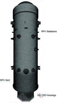
Figure 4. Core shroud and shroud inside.

All the solid elements are assumed to be linear (primary elements). Since the linear tetrahedral element is less accurate than the quadratic element in general, the quadratic tetrahedral element should be used; however, priority over computation time is considered. The authors confirmed that the deformation modes of the results of the FE analysis with the linear tetrahedral element agree well with the results of the LMM analysis, and the accuracy of our analysis was validated. As to the hexahedral elements, the aspect ratio (ratio of the length of the long edge to the short edge) is required to be less than 10 and the incompatible mode element has been assumed. Accuracy of the results is assured as far as possible. The final model has 2,431,695 nodal points, 7,295,085 DOFs and 3,590,592 elements. As can be seen from those indicated figures, the model is large and complex.

The main components are constructed in the following way.

3.4.1. Steam–water separator

The model of the steam–water separator is shown in Figure 5. Solidified 225 stand pipes are divided using the linear hexahedral elements, and tied with the shroud head using multiple-point constraint. The two upper and lower fixing rings are tied with the outermost stand pipes through the brackets. Although the actual stand pipes have fixing rings and fixing rods for preventing from mutual interference, this detailed structure is neglected in the original CAD model. Referring to the results of the eigenvalue analysis with the LMM and the 3D FE analysis by ADVC, the stand pipes have been combined using 25-layered rigid rod elements. This modeling is one of the tuning processes as will be described in Section 3.5. It was hard to construct a 3D FE model compatible to the LMM only through material properties tuning. Though Figure 5 does not show this integrated state, those rigid bars can be seen in Figure 10 that shows the entire FE model.

Figure 5. Construction of steam separator.

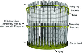
Figure 6. Upper grid plate and fuel assemblies.

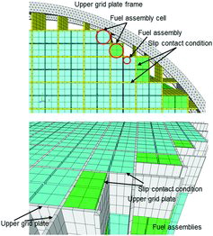
Figure 7. Fuel assemblies, core mounting devices, core support and control rod guide tubes.

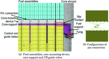
Figure 8. Connection of steam dryer and RPV.

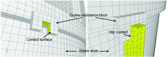
Figure 9. Vibration of CRD housing lower ends through rigid bars and spring elements.

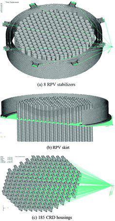
Figure 10. Overall view of FEA model.

3.4.2. Fuel assemblies and the upper grid plate

Figure 6 shows the modeling of the fuel assemblies and the upper grid plate. The fuel assemblies are equipped as four-piece structure except for the outer periphery of the reactor core. Each of these 185 long lattice-shaped structures is called a cell. In the outer periphery, there are 24 cells that equip the only one fuel assembly. Therefore, the total number of the fuel assemblies is 764. The top end of each cell is supported by the upper grid plate. The fuel assembly is so complicated that the shape is rather simplified, and one fuel assembly is constructed with four hexahedral solid elements piled aligned in the axial direction. Slip contact conditions are assigned between the cells and the sides of the upper grid plates. This condition is different from that of the model with the LMM based on the seismic design standard. The effect on the results of 3D analysis different from that of the LMM analysis will be discussed later.

3.4.3. Fuel assembly and fuel support

Configuration of fuel assemblies, fuel support pieces, a core support plate and control rod guide tubes are shown in Figure 7 (see also Figure 4(b)). The number of the control rod guide tubes is 185. The bottom ends of the fuel assemblies are supported by the fuel support pieces, and this support is simulated by pin connection. As shown in Figure 7(b), all the nodal points of the bottom ends of the fuel assemblies are connected to a temporally added nodal point A depicted in this figure by the rigid rods, and all the nodal points of the top end of each fuel support piece are connected to a temporally added nodal point B depicted in this figure by the rigid rods. The translation motion of the nodal points A and B is constrained, while the rotation motion is not constrained. Bending deformation is not transferred from other components to the fuel assemblies and the components under the fuel support pieces by these settings.

3.4.4. Fuel support plate and control rod guide tubes

As shown in Figure 7(a), the fuel support pieces and the control rod guide tubes are connected with the tying (connected contact). The slip contact conditions are defined between the core support plate and the control rod guide tubes.

3.4.5. Control rod guide tubes and control rod drive mechanism (CRDM) housings

Figure 4(b) shows the configurations of the control rod guide tubes and the CRDM housings. Those two components are supported by the pin connection in the same way as the fuel assemblies and the fuel support pieces.

3.4.6. Steam dryer and RPV

The actual steam dryer and the RPV are connected by four quake-resistant blocks on the part of the steam dryer and projection tips on the RPV. The slip contact condition is given as shown in Figure 8, corresponding to this actual state.

3.5. Material properties and tunings for the components

This section describes material properties assumed for the mesh models stated in the previous section. Material properties of each component are shown in Table 1. The RPV main body and the reactor vessel head are made of low alloy steel; the shroud support and the CDR stub tubes are made of inconel; and the steam generator and the core shroud are made of stainless steel. The material constants, Young's moduli, Poisson ratios or mass densities of the various components, are set referring to the data accumulated for the use of the LMM model in the past.

Young's moduli of the fuel assemblies and the control rod guide tubes which were solidified are set so as to have the same value of the product of the Young's modulus and the moment of inertia of area before and after the solidification of those components. Furthermore, for some components that may bring significant effects to the results, the eigenvalue analyses with the LMM and the 3D FE analysis by ADVC have been conducted and the mass densities of those components have been determined. The design earthquake is constructed so as to include frequency component 0.5–50 Hz. Accordingly, in the tuning process, the eigenfrequencies up to 50 Hz are taken into account. Though the detailed description of the tuning is omitted in this paper, the target components that were considered to need the tuning are as follows:

1. fuel assemblies;

2. control rod guide tubes;

3. CRDM housings;

4. RPV;

5. core shroud, upper grid plate and core support plate;

6. core shroud, steam–water separator, upper grid plate and core support plate (added the steam–water separator to (5)).

As an example, the mass density of the RPV is tuned so as to reproduce the first bending mode obtained by the LMM. In addition, some amount of mass is added considering the corresponding components and altitude in order to simulate the reactor water. The authors confirmed that the result of the eigenvalue analysis by the FE analysis coincided well with that of the LMM.

The structural component with the core shroud, the steam–water separator, the upper grid plate and the core support plate given (6) above, was not simulated enough only by tuning the material properties, as stated in Section 3.4.1. After some preliminary analyses and consideration, the 225 stand pipes of the steam–water separator have been connected with the rigid bars in the 25 layers in the upper and lower axial directions in order to match the eigenvalues with the LMM and the FE analysis as far as possible. However, the eigenvalues with the LMM and the FE analysis were 16.4 and 13.0 Hz, respectively, and the sufficient coincidence has not been obtained. This effect will be described later.

3.6. Damping

In the seismic design, the damping factor ζ in the LMM is set for each component, and the damping effect is considered. On the other hand, in the FE analysis, the Rayleigh damping is generally assumed.

The setting method of the Rayleigh damping coefficient for each component is noted as follows. The damping factors are designated not only for the components stated in the previous section as the tuning target components but for all the components for the analysis. Let i be an index that identifies the component. Each component follows the same equation as Equation (6), which is discretized by the FE method: (8) $$M_i{\ddot{u}}_i+C_i{\dot{u}}_i+K_i{u}_i=f_i\left(t\right)$$(8)

First, the equation of undamped free vibration (9) $$M_i{\ddot{u}}_i+K_i{u}_i=0$$(9) is assumed for component i, and the eigenvalue analysis is conducted. From the vibration modes that should be paid attention (only the bending modes in the present analysis) in the frequency range, select the two lowest eigen angular frequencies ω⁽¹⁾_i and ω_i⁽²⁾. The relationships between the Rayleigh damping coefficients α_i, β_i and the eigen angular frequencies are as follows [12]: (10) $$\frac{{\alpha }_i}{{\omega }_i^{\left(1\right)}}+{\beta }_i{\omega }_i^{\left(1\right)}=2{\zeta }_i,\frac{{\alpha }_i}{{\omega }_i^{\left(2\right)}}+{\beta }_i{\omega }_i^{\left(2\right)}=2{\zeta }_i$$(10) where ζ_i is the damping factor of component i. The correspondence between ζ_i and the parameters in the LMM is given as follows: (11) $${\zeta }_i=\frac{c_i}{2\sqrt{m_i{k}_i}}$$(11) where m_i is the mass of the mass point i, k_i is the spring constant and c_i is the damping coefficient. α_i and β_i are obtained by solving Equation (10). C_i in Equation (8) is obtained as follows: (12) $$C_i={\alpha }_i{M}_i+{\beta }_i{K}_i$$(12) which has the same form as Equation (7) in Section 2. This C_i is expanded to the global damping matrix C in Equation (7).

The damping factors in the LMM for the RPV or the core shroud are assumed to be 0.01–0.07. The corresponding Rayleigh damping coefficient α that is proportional to the stiffness is about less than 10⁻⁴, and β that is proportional to the mass is about 0.5–1.3.

3.7. Excitation and constraint

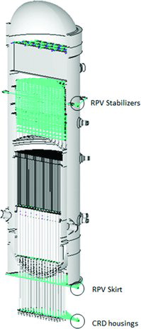
A part of the seismic detector systems is equipped on the foundation slab of the reactor building. The earthquake acceleration is recorded by this detector system. The acceleration on each component is calculated from the observation by the earthquake detector using the LMM for the reactor building and the large coupled system [15,16]. Excitation section is, from above, the eight RPV stabilizers, the bottom of the RPV skirt and the 185 CRDM housing stabilizer restraint beam. These are shown in Figure 3.

The details of the excitation are described as follows. The excitation is given through a bundle of the rigid bars. The respective sections are shown in Figure 9(a)–(c).

See Figure 9(a). The excitation and the constraint on the RPV stabilizers are given as follows. Take a virtual nodal point for the use of the tying (connected contact) assumed on the end section of the stabilizer. All the nodal points are connected by the rigid bar elements. Take another nodal point and connect this point and the tying point by a spring element. The excitation point is connected to the second nodal point noted above. The N, S, E and W accelerations are imposed on the excitation point.

See Figure 9(b). The lower end surface of the RPV skirt is fixed on the RPV support pedestal. All the nodal points of the lower end surface of the RPV skirt are connected to the excitation point. The N, S, E and W accelerations are imposed on the excitation point.

See Figure 9(c). The excitation on the CRDM stabilizer is given as follows. Take rigid bar elements from a nodal point on the upper side of the restraint beams equipped under the 185 CRDM housing stabilizers to a virtual nodal point for the use of the tying connection. Take two other virtual nodal points in the S–N and E–W directions. Connect the virtual nodal point and these two nodal points with the respective spring elements. The accelerations in the S–N and E–W directions are given on these two nodal points.

As for the constraint conditions in the static and the eigenvalue analyses, the excitations by the accelerations are replaced by the zero-displacement constraint conditions.

3.8. FE analysis model

We have now prepared the 3D FE analysis model. See Figure 10. No mesh is presented in this figure. The solid lines that look like cut lines show boundaries between components. A bundle of gray lines in the horizontal direction corresponds to rigid bar elements. The rigid bars omitted in Figure 5 that connect the stand pipes of the steam–water separator are shown in Figure 10. The three circular marks shown in the figure indicate the excitation points stated above.

4. Test analysis

4.1. Unit load analysis

Unit load static analyses in the directions of the x-, y- and z-axes have been conducted using the excitation points shown in Figure 10 as loading points. As an example, Table 2 compares the deadweight and the reaction force, where the acceleration −1G ( = −9.80665 m/s²) in the positive direction of the z-axis has been applied. The evaluation points of the reaction forces correspond to the respective points in Figure 10. This table shows that the reaction forces are evaluated correctly, and the total deadweight is supported by the RPV skirt. The same analyses for x- and y-axes have been conducted and evaluated.

Table 2. Weight of FEA model and reaction forces obtained from the deadweight analysis.

	Weight or reaction
Item	force (kN)
Weight of solid elements	16,636.98
Weight of structural elements	5.93
Added mass in UV direction	2540.83
Reaction force at point 1	0
Reaction force at point 2	−19,183.74
Reaction force at point 3	0
Total	0.00

4.2. Eigenvalue analysis of the whole system

Under the constraint condition noted in Sections 3.4, 3.7 and 3.8, the eigenvalue analysis of the entire reactor system has been conducted. The Rayleigh damping is neglected in this analysis. The slip contact condition is considered here because the condition is infinitesimal and thereby linear.

As noted in Sections 1 and 3, the reactor water has not been simulated and only considered as the added mass given to the RPV and the core shroud. Accordingly, there is a difference between the LMM analysis and the present analysis. The entire component system for comparison with the LMM is the following mechanical system, and we call this entire system the shroud system in this paper:

1. shroud support,

2. fuel assemblies,

3. control rod guide tubes,

4. jet pumps,

5. core shroud,

6. steam–water separator,

7. CRDM housings.

The number of calculated eigenvalues is 250 (1.3–8.0 Hz). Table 3 shows the calculated eigenvalues and those obtained by the LMM analysis mainly of the shroud system. The 1st to 185th eigenmodes correspond to the rotation of the lower ends of pin-connected fuel assemblies and the fuel support pieces (see Section 3.4.3) and Figure 7). The 186th and 187th modes correspond to the first bending modes of the shroud system in the E–W direction (y-axis) and the S–N direction (x-axis), and the eigenfrequencies are 5.8 and 5.9 Hz, respectively. On the other hand, the eigenvalue obtained from the LMM analysis is 8.4 Hz, which is about 30% higher than that of the FE analysis due to the various differences of the modeling stated so far. The 186th and 187th deformation modes are shown in Figure 21(a), which will be referred in Section 6.4. The 188th–195th modes are those of the upper grid plate and the fuel assemblies, and various other modes have appeared in eigenmodes larger than the 195th mode. The eigenvalues of the shroud system and eigenperiods are shown in Table 4. There are some overlappings in Tables 3 and 4.

Table 3. Eigenvalue analysis results of the entire model.

	Eigen		Lumped mass
No.	frequency (Hz)	Mode	model (Hz)
1–185	1.26–1.31	Rotation of fuel assembly	–
186	5.85	E–W bending of shroud system	8.40
187	5.86	N–S bending of shroud system	8.40
188–195	6.80–7.28	Bending of upper grid plate and fuel assembly	–
196–250	7.28–7.99	Bending of CR housing, fuel assembly and various modes	–

Table 4. Summary of eigenvalues and eigenperiods of the shroud system.

	Lumped	Reference
	mass model	case
Eigenvalue (N–S) (Hz)	8.4	5.86
Eigenvalue (E–W) (Hz)		5.85
Eigenperiod (N–S) (s)	0.119	0.171
Eigenperiod (E–W) (s)		0.171

Figure 11. Spectra of the seismic wave in S–N direction translated from calculation time.

Figure 12. Spectra of the seismic wave in E–W direction translated from calculation time.

Figure 13. Mass points of lumped mass model with RPV and the corresponding nodal points of FEM model.

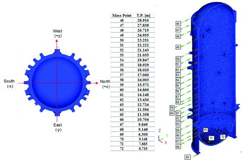
Figure 14. Maximum response accelerations of RPV.

Figure 15. Mass points of lumped mass model with shroud system and corresponding nodal points of FEA model.

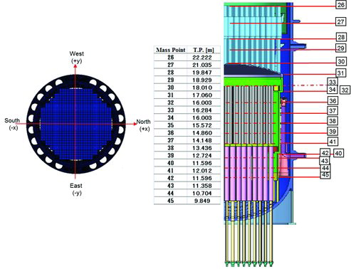
Figure 16. Maximum response accelerations of shroud system.

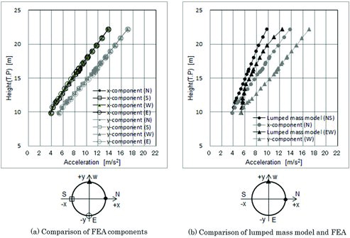
Figure 17. Maximum Mises stress appeared at RPV stabilizer.

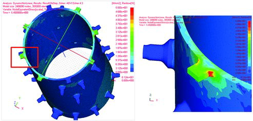
Figure 18. Maximum Mises stress appeared at shroud support leg.

Figure 19. Evaluation positions for relative displacement of core shroud and fuel assemblies.

Figure 20. Maximum relative displacements of fuel assemblies and core shroud.

Figure 21. The 186th eigenmode and deformation response at 6.33 s.

5. Excitation condition, analysis condition and calculation time

The Niigata-ken Chuetsu-Oki earthquake occurred at 10:13 and 23 s on 16 July 2007, and continued 40.96 s. As for the calculation time for the analysis, the period of 12 s from 1.19 to 13.19 s has been taken out. This period includes the maximum acceleration appeared in the whole earthquake event of 40.96 s duration. Table 5 shows the maximum accelerations and the times that bring those accelerations where the start point is assumed to be 0 s instead of the actual point 1.19 s of the target calculation time 12 s. The E–W accelerations (y-axis) are larger than the S–N accelerations (x-axis) for the components given in Table 5, and the maximum accelerations occur on the east side (y-axis negative direction) for each component. Especially, the acceleration as large as 7.14 m/s² (714 gal) occurs on the east side of the RPV stabilizers. As noted in Section 3.7, the accelerations on the RPV stabilizers, the lower end of the RPV skirt and the CRDM housing, and the restraint beams on the CRDM stabilizers have been calculated from the record of the seismic detectors, and those have been imposed on the respective positions as the input earthquake accelerations.

Table 5. Maximum accelerations and their times appeared on vibration points.

			Maximum
		Arrival	accelerations
	Directions	times(s)	(m/s^2)
RPV stabilizers	N–S	6.08	−5.16
	E–W	6.32	−7.14
	U–D	–	–
RPV skirt	N–S	6.48	3.78
	E–W	6.27	−5.48
	U–D	1.41	4.60
CRD housing restraint beams	N–S	6.48	3.78
	E–W	6.26	−5.39
	U–D	–	–

As will be noted in the next section, deviations of the accelerations to the E–W direction bring larger response accelerations of the RPV or the shroud system than those in the S–N direction, and bring larger relative displacements between the fuel assemblies and the core shroud in the E–W direction than the S–N direction.

The vibration response is considered up to about 50 Hz (0.02-s period of time) in the analysis, and Δt has been fixed 0.01 s over the simulation time of 12 s.

The S–N direction earthquake response spectrum over the calculation time of 12 s at the RPV stabilizers is shown in Figure 11(a); the S–N direction earthquake response spectrum over the same calculation time at the restraint beams on the CRDM housing stabilizers is in Figure 11(b). The E–W direction earthquake response spectra over the same calculation time at the same positions are shown in Figure 12. In all those figures, the peak response accelerations can be seen at 0.15 s.

As noted in Section 4.2, the eigenperiods of the 186th and 187th eigenmodes in the FE analysis are nearly equal to 0.17 s. On the other hand, the eigenperiods of the bending modes of the LMM analysis are about 0.12 s. Compared to the eigenperiod of the LMM analysis, that of the shroud system in the FE analysis is closer to the peak earthquake response spectra of 0.15 s as seen in Figures 11 and 12. Due to this reason, the time-dependent response of the shroud system by the FE analysis is considered to be more largely excited than the LMM analysis.

The conducted analysis is a linear response analysis; though a number of contact sections exist, there are little difficulties except for the convergence of the CG method. The computer used is HP BL465c whose node has two sockets of Dual-Core AMD Opteron 2220. The clock is 2.8 GHz; the memory is PC2-5300 DDR2 DIMM 16GB; the communication system is Infiniband; and the operating system is Red Hat Enterprise Linux WS release 4 (Nahant Update 4); the ADVC version is 4.3. The calculation has been conducted with 24 parallel processes using on 6 nodes and 24 cores. The calculation for 12-s event, 1200 steps was 57 days. The calculation time required can be reduced using more cores and parallel processes considering the parallel capability of ADVC. The number of the DOFs is as small as 7.3 million, and the excessive number of the parallel processes brings saturation of the calculation time in general; however, if 256 parallel processes on the same number of cores are supposed to be taken without saturation, the same calculation can be done about five days. The performance of the computer systems is getting higher year by year (e.g. K computer), and there are improvements of the execution environments or usage techniques (e.g. GPU), the calculation time will be able to be reduced soon in the near future.

6. Analysis results

6.1. Maximum response acceleration

In this section, the analysis results with the maximum response acceleration of the RPV and the shroud system obtained by the FE analysis are compared with that of the LMM analysis.

6.1.1. Maximum response acceleration of the RPV

Figure 13 shows sampling positions on the RPV. The sampling mass point numbers in the LMM, and the nodal point positions and those altitudes (T.P., Tokyo Bay Peil. The altitudes from the standard mean sea level in the Tokyo Bay are shown in this figure. The sampling positions are shown in Figure 2. The mass points for comparison are 24 points from 46 to 69. The analysis results are compared on the points in the left side of Figure 13: the south-side end point (the negative position on the x-axis), the north-side end point (the positive position on the x-axis), the east-side end point (the negative position on the y-axis) and the west-side end point (the positive position on the y-axis). Accordingly, 4 × 3 × 24 components can be taken in the FE analysis.

In Figure 14, we compare the maximum response accelerations in the LMM analysis and FE analysis over 12 s in the S–N direction (x-direction) and E–W direction (y-direction) of the RPV. The x- and y-components of the maximum response accelerations on the N, S, E and W end points are depicted in Figure 14(a) along the axis line shown in Figure 13. The x-components of the nodal points along the axis line are almost the same over N, S, W and E. The same tendency is observed in the y-component in Figure 14(a). This means that the accelerations on the RPV occur as the highly rigid cylindrical body and there is little oval-shaped acceleration distribution under the present earthquake acceleration. According to this result, the reference positions in the FE analysis that are compared with the LMM analysis are assumed to be the x-component of the north-side end point in the S–N direction and the y-component of the west-side end point in the E–W direction. Figure 14(b) shows the results of the LMM analysis and FE analysis. Refer to the lower panels in Figures 14(a) and 14(b). Figure 14(b) indicates that the results of both analyses coincide in the S–N and E–W directions, though the FE analysis results are slightly larger than those of the LMM analysis results.

In Figure 14(a), a little variation can be seen in graphs in the S–N and E–W directions (the variation of x- and y-components on the north-side and the south-side end points) at the two altitudes (T.P.) of around 21.14 and 9.85 m. Those two positions correspond to the RPV stabilizers and the shroud support plate, respectively. The latter is an outer disk shown in the left-side figure of Figure 15. The outer surface of the plate is welded on the inner surface of the RPV. Since the RPV stabilizers are the excitation positions, the difference of the accelerations between the S–N and W–E directions is considered to bring this variation. The variation at the position of the stabilizers is considered to be due to a local structure of the RPV. The acceleration variation at the stabilizer position can be seen in Figure 14(b) more clearly. These detailed behaviors can be found only from the 3D FE analysis.

6.1.2. Maximum response acceleration of the shroud system

Figure 15 shows the sampling positions on the shroud system. The corresponding mass points in the LMM analysis are taken to be the mass point number 26–45, totally 20 points, from the upper end of the stand pipe, through the shroud head, to the center of the shroud support body. This figure shows the positions of the corresponding nodal points and those altitudes (T.P.), in addition to the mass point number in the LMM analysis. The mass point numbers in the LMM analysis are also shown in Figure 2. In the same manner as the maximum accelerations on the RPV, totally 4 × 3 × 20 components can be taken in the FE analysis. Although the S–N, E–W and D–U results have been obtained, only the S–N and E–W results are compared in this paper.

In Figure 16, we compare the maximum response accelerations in the LMM analysis and FE analysis over 12 s in the S–N direction (x-direction) and E–W direction (y-direction) of the shroud system. The x- and y-components of the maximum response accelerations on the N, S, E and W end points are depicted in Figure 16(a) along the axis line shown in Figure 15. The x-components of the nodal points along the axis line are almost the same over N, S, W and E. The same tendency is observed in the y-component in Figure 16(a). Figure 16(b) shows the results of the LMM analysis and FE analysis. Refer to the lower panels in Figure 16(a) and 16(b).

In Figure 16(b), the lower starting points in the LMM results and the x-components (S–N components) correspond to the mass point 45, and they are at the center of the axial direction of the shroud support plate. The RPV and the shroud system are connected in this vicinity; therefore, the accelerations of the starting points are equal. As going upward from the mass point 45, the FE analysis results are getting larger than the LMM ones.

Comparing the results of the RPV in Figure 14 and the shroud system in Figure 16, the response accelerations with the RPV by the LMM analysis and FE analysis are almost the same (see Section 6.1.1), whereas the differences between those results of the shroud system seem large. As stated in Sections 3.4.1, 3.5 and 4.2, these differences are considered to be caused by the difference in the eigenfrequencies.

Not only for the shroud system, but also for the RPV stated in the previous section, the response accelerations from the FE analysis are larger than those of the LMM analysis. This can be due to the fact that

1. the reactor water is only considered as the added mass to the RPV and the core shroud, and accordingly, the interaction between components through the reactor water is not included;

2. the eigenperiod from the FE analysis is closer to the peak value of the observed earthquake records than that of the LMM analysis (see Section 4.2).

6.1.2. Maximum stresses

The maximum Mises stresses on each component are shown in Table 6. The Mises stress distributions on the RPV stabilizers and the shroud support legs are shown in Figures 17 and 18. Since the stress values that the LMM evaluates are the primary membrane stress and the primary bending stress [2], there are no stress values in the FE analysis to be directly compared. However, except for the RPV stabilizers and the shroud support legs, the obtained maximum Mises stresses are low on the whole.

Table 6. Maximum stresses on each components.

	Evaluation	Mises
Component	part	stress (MPa)
RPV cylinder body	Body plate	39
	Aseismic block support	97
Lower panel	Welding part of lower panel and RPV body	26
CRDH through-hole	Stab tube	39
Brackets	RPV stabilizer	52
RPV skirt	RPV skirt	114
Shroud support	Welding area	56
Steam dryer	Aseismic block	66
Shroud head	Shroud head	16
Steam separator	Stand pipe	22
Core shroud	Lower body	80
Shroud support	Leg	271
Upper grid plate	Grid	114
Core support plate	Reinforcing beam	122
CRD guide tube	Body	4
Jet pump	Riser brace	17

Comparatively large stress values appear on the RPV stabilizers and the shroud support legs. This tendency agrees with the existing results from the LMM analysis [2]. The high stress values obtained on the shroud support legs are caused by the fact that the fillets that exist on the bases of the legs are omitted (see Figure 18). The actual shape of the fillets can be seen in [17].

6.1.3. Maximum relative displacement of the core shroud and the fuel assemblies

This section describes the maximum relative displacement of the core shroud and the fuel assemblies. The relative displacement of the core shroud and the fuel assemblies in the FE analysis means the differences between the displacements of the core shroud in the horizontal direction and that of the center of the bundle of the fuel assemblies. The relative displacement under seismic condition is important to evaluate the control rod insertion [18].

Figure 19 shows sampling positions. The table placed in the center of Figure 19 shows seven mass points and their altitudes (T.P., see Section 6.1.1). The number of the corresponding nodal points in the FE analysis is 16. In the LMM, the fuel assemblies and the center of the core shroud are compared.

Figure 20 compares the results of the LMM analysis with that of the FE analysis of the maximum relative displacement of the core shroud and the fuel assemblies over 12 s in the N–S direction (x-direction) and the E–W direction (y-direction). Figure 20(a) depicts the x- and y-components in the outermost positions of the N, S, E and W along the axis line shown in Figure 19. Figure 20(b) shows the results of the LMM analysis and FE analysis. Refer to the lower panels in Figure 20(a) and 20(b). We can conclude from Figure 20 the following properties:

1. In the FE analysis, Figure 20(a) shows that the results of the x-components in the N, S, E and W directions almost coincide. The same tendency can be observed in the y-components.

2. In the FE analysis, Figure 20(a) shows that the maximum response displacements in the E–W direction (y-axis direction) are larger than those in the S–N direction (x-axis direction).

3. Figure 20(b) shows that in the result of the LMM analysis the response displacements in the E–W direction (y-axis direction) are larger than those in the S–N direction (x-axis direction). Those are due to the deviation of the earthquake acceleration stated in Section 5 (the E–W acceleration is larger than the S–N), Figure 20(b) shows that the maximum relative displacements from the LMM analysis are larger than those of the FE analysis. As stated in Section 3.4.2, since the upper and lower ends of the fuel assemblies are pin connected in the LMM analysis, the rotation is not constrained, and so is the bending in the S–N and E–W directions; on the other hand, in the FE analysis, the lower ends of the fuel assemblies are pin connected and the slip condition is assumed in the upper ends. Thus, in the FE analysis, the fuel assemblies can move up and down, but are hard to move in the bending direction due to the stiffness of the upper grid plate. This indicates that there is a possibility of excessive conservatism in the LMM analysis.

6.1.4. Results of eigenvalue analysis and time-dependent response displacements

As stated in Section 4.2, the bending modes appear in the 186th and 187th modes, and these two correspond to the E–S (the y-axis direction) and the S–N directions, respectively. This section describes how the bending modes of the shroud system are related to the time-dependent response displacements.

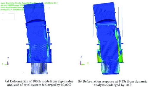
As stated in Section 4.2, the 186th and 187th eigenfrequencies are roughly 5.8 Hz, and eigenperiods are 0.17 s. The 186th modal diagram in the E–S direction is shown in Figure 21(a). The deformation is enlarged by 30,000, and the color contour indicates an equivalent stress distribution.

On the other hand, as stated in Section 5, the earthquake response spectrum of each component has a peak at 0.15 s that is close to 0.17 s. The maximum response spectrum of the shroud system over 12 s was stated in Section 6.1.2. Separating those 12 s into small time periods, transitions of the response acceleration are obtained and shown in Figure 22. Each curve corresponds to the maximum response in the time interval from 0 s to the respective time indicated in this figure. From this figure, the response accelerations reached the maximum level at 6.33 s over a total of 12 s. In this figure, the results of the LMM analysis (see Figure 16) are superimposed. The FE analysis results come to the same level of the LMM model at 6.3 s, and grow largely over the LMM results immediately afterwards.

Figure 22. Time-dependent response accelerations of shroud system at north-side y-component.

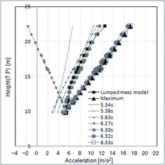
The deformation response at 6.33 s is shown in Figure 21(b), where the deformation is enlarged by 100 and the contour indicates the equivalent stress distribution in the same manner as in Figure 21(a). Comparing Figure 21(a) and 21(b), the deformation of the shroud system in (b) closely resembles to the modal deformation shown in (a); therefore, the deformation response at 6.33 s is considered to be excited by the earthquake spectrum at around 0.15 s.

Figure 21(a) and 21(b) is an example of 3D visualization, as well as Figures 17 and 18. The authors have made motion pictures or walk-through visualization (which is similar to a visualization with a moving viewpoint with a video camera) from the 3D analysis results, though no shots are shown in this paper.

The difference in the results between the LMM analysis and FE analysis results nearly in the difference between the eigenfrequencies of the LMM analysis and FE analysis. The fact that the FE analysis does not include the reactor water may bring some of the differences of the eigenfrequencies.

7. Conclusions

The authors have conducted the seismic analysis using the 3D FE analysis of the BWR5-type boiling water reactor, and described in this paper. The used data and the evaluation of the analysis results referred to the seismic design standard and the LMM analysis that follows this standard. What has been described in this paper can be summarized as follows:

1. In the process of construction of the CAD model, the components such as the steam–water separator or the fuel assemblies which have especially complicated shapes or structures, the models have been simplified to some extent. In the process of mesh generation, some cylindrical components such as the fuel assemblies have been solidified (Section 3.3).

2. Long cylindrical components such as the fuel assemblies or the control rod guide tubes have been divided by the hexahedral elements as far as possible so as to reduce the number of the nodal points. Complicated components that include curved surface such as the RPV have been divided by the tetrahedral elements. The used elements are tetrahedral, hexahedral and pentahedral elements. All these elements are assumed linear due to the restriction of calculation time. The hexahedral elements used are the incompatible mode elements (Section 3.4).

3. The material properties have been defined referring to the design values. As to the difference of the components from the design due to solidification, the properties have been tuned referring to the results of the LMM analysis. The Rayleigh damping has been defined to each component based on the respective eigenvalue analysis. The reactor water has not been considered directly, but included as the added mass to the RPV and the core shroud (Section 3.5).

4. Although the design standard prescribes the top and bottom ends of the fuel assemblies, and is supported by the pin connection on the upper grid plate and the fuel support pieces, the contact condition has been assumed on the fuel assemblies and upper grid plate in the FE analysis (Section 3.4.2, see Figure 6).

5. The tying connection, the slip contact, the beam elements and the rigid beam elements have been used for the connection of the components. The excitations have been applied in the following way: the RPV stabilizers are excited through the rigid bars and the spring elements; the RPV skirt has been excited through the rigid bars; and the restraint beams on the CRDM housing stabilizers have been excited through the rigid bars and the spring elements (Sections 3.4 and 3.7).

6. From the record of the Niigata-ken Chuetsu-Oki earthquake, 12-s acceleration from 1.19 to 13.19 s that includes the maximum acceleration has been taken out and applied to the excitation positions. The peak values of the spectra of the earthquake acceleration at the corresponding positions can be seen at 0.15 s (Section 5; Figures 11 and 12).

7. The used analysis code is ADVENTURECluster that can be applicable to large-scale analyses. The number of the nodal points is 2,431,695, that of the DOFs is 7,295,085 and that of the elements is 3,590,592. The used machine is a standard cluster system with 6 nodes and 24 cores. The number of the parallel processes is 24 (Sections 2 and 5).

8. The time-dependent analysis is conducted over 12 s noted (6) above. The calculation time is 57 days. By increasing the number of the parallel processes or by other measures, this calculation time could be largely reduced.

9. The targets for comparison with the the LMM analysis are the maximum response accelerations of the RPV and the shroud system, and the maximum response relative displacements between the fuel assemblies and the core shroud. Though the maximum response accelerations of the RPV have agreed well with the results of the LMM, some differences of the maximum response accelerations of the shroud system have been found. The maximum stresses of the FE analysis have almost agreed with those of the LMM analysis. The maximum response relative displacements between the fuel assemblies and the core shroud from the FE analysis have been rather small compared with those of the LMM analysis. This is considered to be due to the difference of the support mechanism of the fuel assemblies noted (4) above (Sections 4.1 and 4.3).

10. The maximum response accelerations of the shroud system by the FE analysis have been larger than those of the LMM analysis. This is considered to be due to the fact that the eigenperiod of the FE analysis is closer to the peak value of 0.15 s of the earthquake acceleration spectrum than the LMM results (Section 6.4).

11. 3D visualizations have been conducted as in the various figures in this paper.

As has been stated, the seismic design and the LMM analysis results have been roughly reproduced from the FE analysis. On top of that, some problems have been found in the construction of the 3D FE model. First, improvement of modeling method and parameter tuning for vibration characteristics in the FE analysis are needed. Second, we need inclusion of the effect of the reactor water, especially, interactions of the components through the reactor water, both of which affect the vibration characteristics of the components. In the seismic analysis, modeling of the vibration characteristics is especially important. Since the existing LMM has been used for the seismic design of the nuclear power plants for a long time as the standard method, it has a high-level credibility. However, if we can resolve each of the problems in the FE analysis as has been noted above and described so far in this paper such as modeling method, reduction of calculation time or handling of the large data, the FE analysis has potential as a valuable tool. Characteristics of the 3D FE analysis can be summarized and renewed as follows:

1. Detailed modeling and precise evaluation become possible not depending on experience and intuition.

2. We enable to capture intuitive 3D behaviors of various parts.

3. 3D behavior is not only easy to evaluate but also helpful to explain to third party.

4. Reuse of the 3D CAD model for design to the analysis model can be possible (see Figure 1).

5. Circumferential asymmetry of the configuration of the model can be considered (see Figures 13 and 15).

6. Circumferential asymmetry of the boundary conditions or operation conditions can be considered.

7. Spatial nonuniformity of the input earthquake motion can be considered as a special case of (6) above. In our study, however, on the RPV stabilizer, the RPV skirt and the restraint beams on the CRDM are only vibrated in the E–W, S–N and D–U directions.

In addition to those above, the fact that the material nonlinearity and the geometric nonlinearity can be considered without special measures will be a large advantage of the FE analysis. In our study, the analysis has been assumed to be linear, and has been focused on the results in the S–N and E–W directions in order to compare with the results of the LMM analysis. As far as the linear analysis is concerned, the response in the arbitrary direction can be obtained by the linear combination of the results of the S–N and E–W directions (or the results of the S–N, E–W and D–U directions) by the LMM analysis in theory. However, in order to grasp the behavior with the 3D extension keeping the nonlinear analysis open, the FE analysis is the valid analysis methodology. The authors are hoping to make use of the 3D FE analysis in various areas including the seismic analyses of the nuclear power reactors.

Acknowledgements

Our work was conducted cooperatively with a team consisting of many engineers and researchers. The authors would like to thank Kenji Murano, Kazuyuki Nagasawa, Masashi Fukushima, Takehiro Oku, Yoshio Takagi and Ai Watanabe (Tokyo Electric Power Company); Masaaki Tanaka, Yuichi Sawahata and Minoru Otaka (Hitachi-GE Nuclear Energy); Tetsuya Wada, Takayuki Hayashi, Kunizo Onda, Yoshikazu Katai and Koji Nishimoto (Allied Engineering Corporation); and Shin-ichiro Sugimoto and Hiroshi Kawai (The University of Tokyo) for their efforts.

References

- Nuclear and Industrial Safety Agency. Report on the facility soundness evaluation of Unit 7 of TEPCO's Kashiwazaki-Kariwa Nuclear Power Station. Tokyo (Japan): NISA; 2009. Japanese.
- Nuclear and Industrial Safety Agency. Report on the aseismic reliability evaluation of Unit 5 of TEPCO's Kashiwazaki-Kariwa Nuclear Power Station under the revision of the seismic design standard. Tokyo (Japan): NISA; 2010. Japanese.
- Oku T, Akiba H, Suzuki S, Yoshimura S. Seismic response analysis using three dimensional FEM analysis for BWR nuclear reactor facilities. Proceedings of SNA + MC2010; 2010 October 17–21; Tokyo, Japan.
- Akiba H, Kobayashi K, Suzuki S, Yoshimura S. Large scale parallel structural analysis system and its application to seismic analysis of BWR. Proceedings of SNA + MC2010. 2010 October 17–21; Tokyo (Japan).
- Fukushima M, Akiba H, Suzuki S, Yoshimura S. Seismic response analysis of BWR pressure vessel and core internals using three dimensional finite element method - The behavior during earthquake and evaluation of the design margin using three dimensional detailed model -. 2011 Annual Meeting of the Atomic Energy Society of Japan; 2011. Japanese. ISBN:978-4-89047-151-5.
- Akiba H, Fukushima M, Suzuki S, Yoshimura S. Seismic response analysis of BWR pressure vessel and core internals using three dimensional finite element method - large scale structural analysis system and its application to seismic analysis of nuclear reactor -. 2011 Annual Meeting of the Atomic Energy Society of Japan; 2011. Japanese. ISBN:978-4-89047-151-5.
- Suzuki S, Akiba H, Fukushima M, Yoshimura S. Seismic response analysis of BWR pressure vessel and core internals using three dimensional finite element method -development for advanced three dimensional FEM model considering design concept of seismic response analysis -. 2011 Annual Meeting of the Atomic Energy Society of Japan; 2011. Japanese.
- Allied Engineering Corporation. Available from: http://www.alde.co.jp/.
- ADVENTURE Project website. Available from: http://adventure.sys.t.u-tokyo.ac.jp/.
- Kataoka S, Minami S, Kawai H, Yamada T, Yoshimura S. A parallel iterative partitioned coupling analysis system for large-scale acoustic fluid–structure interactions. Comput Mech. 2014;53:1299–1310.
- Suzuki M, Ohyama T, Akiba H, Noguchi H, Yoshimura S. Development of fast and robust parallel CGCG solver for large scale finite element analyses. Trans Jpn Soc Mech Eng Series A. 2002;68:1010–1017. Japanese.
- Bathe K. Finite element procedures. Upper Saddle river, NJ: Prentice Hall; 1967.
- Akiba H, Ohyama T, Shibata Y, Yuyama K, Katai Y, Takeuchi R, Hoshino T, Yoshimura S, Noguchi H, Gupta M, Gunnels J, Austel V, Sabharwal Y, Garg R, Kato S, Kawakami T, Todokoro S, Ikeda J. Large scale drop impact analysis of mobile phone using ADVC on Blue Gene/L [CD-ROM]. Proceedings of SC06; 2006 November 11–17; Florida.
- Akiba H, Miyamura T, Ohsaki J, Kohiyama M, Yamashita T, Hori M, Kajiwara K. Numerical shaking table E-Simulator and its hybrid parallelization, Proceedings of the Annual Meeting of The Japan Society for Industrial and Applied Mathematics; 2011 September 14–16; Kyoto (Japan). Japanese.
- Japan Electric Association.Technical guidelines for aseismic design of nuclear power plants, expanded edition. Japan: Japan Electric Association; 1987. Japanese. ( JEAG4601-1987).
- Japan Electric Association. Technical Guidelines for Aseismic Design of Nuclear Power Plants Supplement. Japan: Japan Electric Association; 1991. Japanese. ( JEAG4601-1991).
- Ogawa K. Study on residual stress and fracture evaluation. Tokyo (Japan): Japan Nuclear Energy Safety Organization (JNES); 2009. Japanese.
- Current status of verification test for nuclear power facility. Japan: Nuclear Power Engineering Test Center and Japan Power Engineering and Inspection Corporation; 1988. Japanese.
- Jamet P, Godoy R, Gunssel L, Gürpinar A, Johnson J, Kostov M. Mission report, Volume 1 and 2: Preliminary findings and lessons learned from the 16 July 2007 earthquake at Kashiwazaki-Kariwa NPP. Department of Nuclear Safety and Security, Vienna (Austria): IAEA; 2007.