Study on computational performance in generation of cross sections for nodal simulators using continuous-energy Monte Carlo calculations

Abstract

This paper aims to evaluate the practical feasibility of using the continuous-energy Monte Carlo method for producing homogenized group constants for deterministic core simulators. The calculations are carried out using the Serpent 2 Monte Carlo code and ARES nodal diffusion fuel cycle simulator. A test case from a previous validation study is repeated with varying number of neutron histories in group constant generation. The impact of statistical variation in the results of ARES simulations is evaluated, and the corresponding calculation times used to provide an order-of-magnitude estimate for the overall computational cost for generating the full set of group constants covering all state points. It is concluded that, while computationally expensive, Monte Carlo-based spatial homogenization involving burnup and thousands of state points per assembly type is within the range of feasibility using modern computer clusters.

Keywords:

• serpent
• ARES core simulator
• Monte Carlo
• group constants
• statistics
• computational cost

1. Introduction

The use of the continuous-energy Monte Carlo method for spatial homogenization has been studied since the 1980s, and it started becoming a popular research topic at around year 2000, along with the development of calculation codes and computer capacity. The motivations driving this work include the method's capability to handle complicated geometries using the best available knowledge on neutron interactions without major approximations. The fact that the transport simulation is inherently three-dimensional (3D) makes it possible to grasp the effects of axial heterogeneities, when moving from two-dimensional to 3D methods in spatial homogenization. This capability makes continuous-energy Monte Carlo the method of choice for the modeling of various novel reactor concepts, such as resource-renewable boiling water reactors (RBWRs), aiming for high conversion ratio by axial division of fuel assemblies into separate seed and blanket zones.

One of the first Monte Carlo codes specifically intended for this task is Serpent,developed at VTT Technical Research Centre of Finland since 2004. Spatial homogenization still remains an important topic for future work, and one of the near-term goals involves creating an independent calculation system for the safety analyses of Finnish power reactors. The work is carried out within the framework of a national research programme on nuclear power plant safety (SAFIR2014), and in addition to Serpent, this work includes deterministic fuel cycle and transient simulator codes developed at VTT and the Finnish Radiation and Nuclear Safety Authority (STUK) over the years: AFEN REactor Simulator (ARES), TRAB3D, HEXBU3D and HEXTRAN.

Validating each coupled code sequence forms a major part of this task, and the work began in 2013 with the ARES core simulator. The first phase of the study [1] involved hot zero-power initial core calculations, using the MIT BEAVRS Benchmark [2] as the test case. The results showed that the Serpent-ARES calculation sequence was capable of reproducing the results of a 3D Monte Carlo reference solution with good accuracy at both assembly and pin level. The next phase of the validation study extends the calculations to full power and burnup, which considerably complicates the task of group constant generation.

Before proceeding forward, it was decided to take a closer look at the scale of this task. Even though it has been shown that the Monte Carlo method can be used for group constant generation, this task has not yet been put to practice in full scale, and there are several questions remaining unanswered.

(i)	What is the impact of statistical error in group constants in the results of the full-core simulation, or more precisely, what is the acceptable level of statistical error in Monte Carlo transport calculation?
(ii)	What is the impact of statistical error in transmutation cross sections used in burnup calculations, or more precisely, what is the acceptable level of statistical error in Monte Carlo burnup calculation?
(iii)	How many neutron histories need to be run to reach an acceptable level of statistical accuracy?
(iv)	What is the overall computational cost of producing the full set of group constants with Monte Carlo-based homogenization?

This paper aims to address these questions without actually going the full distance. The previous calculations presented in Ref. [1] are repeated with different number of neutron histories, and the impact of statistical variation in the full-core ARES simulations evaluated by comparison to a 3D Monte Carlo reference solution. The running times from corresponding representative assembly burnup calculations are then used for extrapolating the overall computational cost of full-scale group constant generation, covering all state points within the operating cycle.

The methods used in the ARES core simulator and for group constant generation in Serpent 2 are briefly described in Section 2. The test case is introduced in Section 3, with a revisit of the results of the previous study [1]. The four questions listed above are addressed in Section 4.

2. Methods

2.1. ARES core simulator

ARES [3], is a 3D LWR core simulator, developed since 2000 at the Finnish Radiation and Nuclear Safety Authority (STUK), mainly for the purpose of independent safety analyses of Finnish power reactors. The code can be used for stationary fuel cycle simulations of PWR and BWR cores with rectangular fuel geometry. The applications of ARES include evaluation of safety margins, burnup calculations for transient analyses and reference calculations for commercial reactor simulator codes.

The neutronics solution in ARES is based on the two-group nodal diffusion method and a 3D analytical function expansion nodal model (AFEN). The two-group nodal flux solution is written in eigenmode representation, using 18 analytical form functions per flux mode. The large number of form functions offers improved modeling of diagonal flux tilts between assemblies and better accuracy near assembly edges, which is directly reflected in the accuracy of pin-power reconstruction. The flux solutions between nodes are coupled together radially using eight discontinuity factors per group, one for each assembly boundary and edge.

Fuel cycle simulations involve the modeling of core neutronics subject to slow changes in reactor operating conditions, such as power output, reactivity control and fuel burnup. The group constants used for forming the nodal diffusion equations are obtained by interpolation and polynomial fits between tabulated state points.

2.2. Group constant generation in Serpent 2

The homogenized two-group constants read by ARES include absorption, fission, fission neutron production, fission energy production and scattering removal cross sections, diffusion coefficients and poison production and absorption cross sections for ¹³⁵Xe, ¹⁴⁹Sm and their precursors. Serpent uses built-in methodology for obtaining these constants from the continuous-energy Monte Carlo simulation. In the simplest case, the homogenized fuel assembly is surrounded by reflective boundary conditions, and the calculation of two-group cross sections and diffusion coefficients is carried out in two steps. First, homogenized reaction cross sections are calculated with standard flux and reaction rate tallies using an intermediate multi-group structure, typically consisting of 40–70 energy groups. This data are then collapsed into two energy groups, using either the infinite spectrum from the Monte Carlo calculation, or a critical spectrum obtained by solving the B₁ equations. This approach allows performing a leakage correction on the homogenized cross sections [4], and consistent flux weighting for the diffusion coefficients [5].

If the homogenized region is surrounded by reflective boundary conditions, the calculation of assembly discontinuity factors (ADFs) can be accomplished using conventional cell and surface flux tallies. If this is not the case, the procedure requires an explicit solution for the local homogeneous flux, using the non-zero net currents as boundary conditions. In this study, this procedure was carried out using a Matlab script, as described in Ref. [1], but the methodology has been later implemented in Serpent 2 as an internal subroutine. Situations calling for an explicit solution for the local homogeneous flux include reflectors, in which the entire source term is provided by a non-zero net current from the adjacent fuel assemblies. Similar condition arises when the homogenized assembly is modeled with its surroundings, which is sometimes necessary to account for steep flux gradients resulting from strong absorbers or positioning of the assembly in the reactor core, for example, at the core-reflector boundary. The homogeneous flux solution is used not only for the calculation of ADFs, but also for energy group-wise form factors used for pin-power reconstruction.

3. Test case and previous calculations

The MIT BEAVRS Benchmark [2] was established in 2012 for the purpose of providing a test case for the validation of high-fidelity core analysis methods, such as 3D continuous-energy Monte Carlo. The benchmark consists of a detailed description of a commercial 1000 MW Westinghouse PWR reactor core, including operating history for the first two cycles. The hot zero-power state of the initial core was modeled using ARES, with Serpent-generated group constants. Serpent was also used to provide a full-scale 3D reference solution for the ARES simulations. All Monte Carlo calculations were run with a very large number of neutron histories, in order to minimize the impact of statistical variation in the results.

The results turned out to be in good agreement at both assembly and pin-level [1]. Differences in radial assembly-wise power distributions ranged from −1.6% to 0.6% at core mid-plane, and the reconstructed pin-powers were off by less than 1% in 82% of all fuel pins. Axial power distributions were also in good agreement, and the dominating error source was the local depression in thermal flux caused by grid spacers, which in the ARES model were homogenized in the group constants.

The results also showed that the ARES solution is particularly sensitive to ADFs, which in turn depend on the geometry in which the homogenization is performed. It turned out that the calculation failed completely if all assemblies were homogenized in single-assembly calculations with reflective boundary conditions. Closer analysis showed that the main reason for the poor results was a single assembly type located at the core-reflector boundary, with six burnable absorber pins positioned asymmetrically on the half facing the inner core. When this assembly was homogenized in a geometry containing its immediate surroundings, the results were considerably improved. Nevertheless, attaining the ∼1% accuracy at pin-level required abandoning the simple approach for all assembly types, and performing the calculations in a geometry containing 2.5 assembly widths of neighbors surrounding the homogenized assembly.

4. Results

Even though the previous calculations showed that the best results are obtained by including a sufficiently large region of surroundings in the geometry where the homogenization is performed, this approach cannot be considered practical for several reasons. First, extending the geometry in all directions means that the number of tally scores in the homogenized assembly is reduced, which in turn may translate into a considerable increase in running time. Second, the surroundings can be different for the same assembly type in different positions, which increases the total number of runs. Finally, the position of the assembly changes after each reload. Since the local environment can have an impact on how the assembly is depleted, it might become necessary to include the surroundings in the parametrization of group constants as an additional history variable.

Instead of taking the best model from Ref. [1] as the basis of this study, it was decided to make a compromise between accuracy and complexity. The two assembly types located in region 3 at the core-reflector boundary with 3.1 wt-% enriched fuel without burnable absorber and with six asymmetrically positioned absorber pins were homogenized with a half assembly width of surroundings, while a single-assembly model with reflective boundary conditions was used for the rest.This allowed the number of assembly types to remain at nine, with a relatively simple procedure for homogenization. Using the less refined model increased the maximum errors at mid-plane assembly powers to about 3%, compared to the reference 3D Monte Carlo calculation.

4.1. Impact of statistics in homogenization

To assess the impact of statistical variation in the Monte Carlo-based homogenization and the results of full-core ARES calculations, 20 independent sets of group constants were produced for the HZP initial core configuration. The calculations were repeated with 1, 5, 10 and 50 million neutron histories, and some average values and relative standard deviations for a representative fuel assembly are presented in Table 1. It is seen how increasing the number of neutron histories reduces the statistical variation.

Table 1. Selected group constants (absorption, fission neutron production and scattering removal cross sections, diffusion coefficients and surface and corner ADFs) for a representative fuel assembly (2.4 wt-% ²³⁵U fuel with 12 burnable absorber pins). The results are mean values and the associated relative standard deviations (in percent) from 20 independent runs.

Param.	Number of active neutron histories per run
	1,000,000	5,000,000	10,000,000	50,000,000
Σa, 1	8.904E−03 (0.147)	8.907E−03 (0.039)	8.906E−03 (0.044)	8.905E-03 (0.014)
Σa, 2	8.381E−02 (0.050)	8.381E−02 (0.037)	8.380E−02 (0.020)	8.380E−02 (0.009)
νΣf, 1	5.347E−03 (0.090)	5.345E−03 (0.050)	5.345E−03 (0.037)	5.345E−03 (0.018)
νΣf, 2	1.019E−01 (0.066)	1.019E−01 (0.048)	1.019E−01 (0.026)	1.019E−01 (0.010)
Σs, 1 → 2	1.834E−02 (0.063)	1.834E−02 (0.028)	1.835E−02 (0.021)	1.835E−02 (0.012)
D1	1.397E+00 (0.066)	1.397E+00 (0.022)	1.397E+00 (0.013)	1.397E+00 (0.006)
D2	3.933E−01 (0.043)	3.933E−01 (0.017)	3.933E−01 (0.010)	3.933E−01 (0.006)
$F_1^{\mathrm{s}}$	9.945E−01 (0.170)	9.946E−01 (0.063)	9.948E-01 (0.043)	9.947E−01 (0.018)
$F_2^{\mathrm{s}}$	1.062E+00 (0.387)	1.061E+00 (0.148)	1.061E+00 (0.096)	1.060E+00 (0.057)
$F_1^{\mathrm{c}}$	9.994E−01 (0.461)	9.985E−01 (0.179)	9.984E−01 (0.202)	9.985E−01 (0.064)
$F_2^{\mathrm{c}}$	1.090E+00 (1.389)	1.089E+00 (0.446)	1.091E+00 (0.393)	1.089E+00 (0.130)

The largest deviations are found in the ADFs, especially the corner values. The reason is that the surface flux tallies used for calculating the ADFs are scored only when the neutron is reflected from the boundary, while scores for the homogenized cross sections are made for each collision.The corner ADFs are calculated using a surface flux tally on a segment extending 5% of the assembly width in the direction of both faces. The symmetry of the assembly allows averaging the values over all surfaces and corners, which improves the statistics. Enforcing symmetry for the ADFs of symmetrical assemblies is important also because the same values are used for multiple nodes in the core model, and the amplification of small statistical variations would lead to a radial flux offset and systematic error.

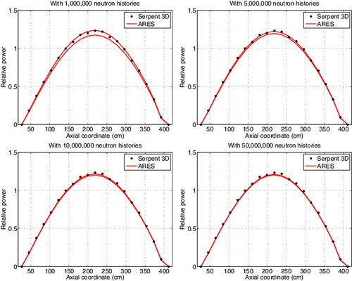
The 20 independent sets of group constants were used to run 20 independent ARES simulations. The maximum relative errors in core mid-plane assembly powers compared to a 3D Monte Carlo reference solution are presented in Figure 1.When the group constant data is produced with only one million neutron histories, the maximum errors are in the order of 5%. The worst calculation case shows a considerable offset in the radial power distribution, with an under-prediction at core center and over-prediction at the periphery. The results are gradually improved as the number of histories is increased. Going beyond 50 million histories showed practically no improvement, which suggests that the impact of statistical variation is well below the errors resulting from approximations and methodological factors, such as the geometry used in the homogenization of fuel assemblies and reflector nodes. Even the differences between results obtained with 10 and 50 million histories are barely noticeable. Similar comparison for axial power distributions showed very similar results. Differences in the central assembly position are plotted in Figure 2.

Figure 1. Maximum errors (in %) in radial power distributions at core mid-plane, compared to reference 3D Monte Carlo calculation. The color scale and the top value show the maximum error, and the bottom value the relative standard deviation calculated from 20 independent ARES simulations.

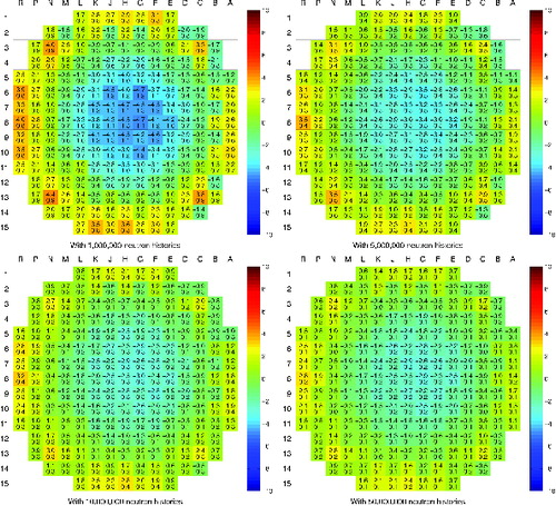
Figure 2. Axial assembly-wise power distributions at core center. The solid curves show the minimum and maximum result from 20 independent ARES runs.

4.2. Impact of statistics in burnup calculation

To see how statistical variation affects the evolution of material compositions, and consequently, group constants at higher burnup, 20 independent assembly burnup calculations were performed for selected assembly types. The fuel was irradiated to 60 MWd/kgU burnup, with the depletion history described in detail in the following section. Each fuel pin was handled as a separate depletion zone, and the procedure was again repeated using 1, 5, 10 and 50 million neutron histories.

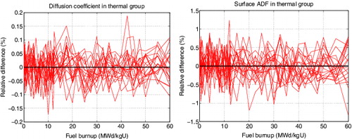
The results showed that the standard deviations in group constants remained at the same level as the fuel was burnt, and the propagation of statistical error seemed to cause no observable systematic deviation from the mean value, even with the lowest number of neutron histories.The random behavior is illustrated for a representative fuel assembly (2.4 wt-% ²³⁵U fuel with 12 burnable absorber pins) in Figure 3, in which the results from calculations with 1 million neutron histories are compared to the average of calculations with 50 million neutron histories. Similar behavior was observed for the other group constants as well.

Figure 3. Thermal group diffusion coefficient and surface ADF from 20 independent runs with 1 million neutron histories, compared to corresponding average of 20 independent runs with 50 million neutron histories. The differences show random oscillation without any systematic trend as function of burnup.

4.3. Estimation of overall computational cost

In order to generate group constants for a fuel cycle simulator calculation, the values need to cover all operating conditions within the reactor core throughout the simulated cycle or cycles. In the simplest case, this means the range of core temperatures and burnup from fresh fuel to discharge, together with reactivity control, which in the case of a PWR means control rods and boron shim. Simulation of reactor start-up and shut-down requires data for the hot zero-power state, and the evaluation of safety margins extends the calculations beyond normal operating conditions. The group constant data is parametrized according to discrete state-points, and the local values for the nodal solution are interpolated from the state-point matrix based on the operating history and the iterative solution between neutronics and thermal hydraulics.

Since the local operating conditions inside a fuel assembly also affect how the assembly is depleted, the state-points by which the group constant data is parametrized are not completely independent. The calculations are instead divided into:

(1)	History cases, which take into account variables related to operating conditions that persist for an extended period of time and affect how the fuel is depleted, for example, coolant density, temperature and boron concentration.
(2)	Branch cases, which take into account variables related to momentary changes in the operating conditions, for example, insertion of control rodsor increase or decrease in fuel temperature.

In practice, group constant generation involves running assembly burnup calculations covering all assembly types and history case variables. Branch case variables are accounted for by performing restart calculations for each burnup point, varying the local operating conditions accordingly.

The estimation of computational cost for producing the full set of group constants for ARES fuel cycle simulations was based on a representative assembly burnup calculation (2.4 wt-% ²³⁵U fuel and 12 burnable absorber pins), from which the overall calculation time was extrapolated by multiplying with the number of fuel assemblies and history cases, taking into account the number of branches. The estimate is essentially based on the following assumptions:

(i)	All transport calculations are run with the same number of neutron histories and all burnup calculations with the same number of steps.
(ii)	Burnup calculation time is the same for all assembly types and history conditions.
(iii)	Calculation time for a single branch case is the same as the average time taken over the branches of a representative burnup calculation.

The variables used for determining the total number of history cases are listed in Table 2. The combinations of 9 assembly types, 3 moderator temperatures and 3 boron concentrations results in a total of 9 × 3 × 3 = 81 burnup simulations. For each history case, a number of branch calculations are assumed to be run for different burnups, as listed in Table 3. The total number amounts to 16 × 3 × 3 × 3 − 16 = 416, without accounting for the insertion of control rods. Control rods can be inserted in 3 of the 9 assembly types, which adds 16 × 3 × 3 × 3 = 432 branches in 3 × 3 × 3 = 27 history cases. The total running time can be estimated from (1) $$\begin{array}{ccc}\hfill T_{\mathrm{tot}}& =& 81\times T_{\mathrm{burn}}+(81\times 416+27\times 432)\times T_{\mathrm{bra}}\hfill \\ & =& 81\times T_{\mathrm{burn}}+45360\times T_{\mathrm{bra}},\hfill \end{array}$$(1) where T_burn and T_bra are the estimated running times for a single burnup calculation and transport branch, respectively. The representative burnup calculations were run with 12 CPU cores on a 3.47 GHz Intel Xeon X5690 workstation. The calculation times, together with the estimated totals are summarized in Table 4.

Table 2. Assembly types and variables used to determine the number of history cases.

	No.	Values
		1.6 wt-% ^235U (no BP pins); 2.4 wt-% ^235U
Fuel assembly types	9	(0/12/16 BP pins); 3.1 wt-% ^235U (0/6/15/16/20 BP pins)
Moderator temperature and density	3	Core inlet; average; core outlet
Boron concentration	3	Beginning of cycle; cycle average; end of cycle

Table 3. Burnup points and variables used to determine the number of branch cases.

	No.	Values
Burnup points	16	0; 0.1; 1; 3; 5; 7; 9; 10; 11; 12; 15; 20; 30; 40; 50; 60 MWd/kgU
Fuel temperature	3	Nominal; core inlet (zero power); elevated
Moderator temperature	3	Nominal; high; low
Boron concentration	3	Nominal; high; low
Control rods	2	Withdrawn; inserted

Table 4. Total and single transport calculation running times for the representative fuel assembly (2.4 wt-% ²³⁵U fuel with 12 burnable absorber pins), together with the estimated total running time required for producing the full set of group constants. All calculations were run with 12 CPU cores.

Neutron	Running times (min)		Estimated
histories	Tburn	Tbra	total (days)
1M	30.5	0.5	18.5
5M	91.5	1.8	62.8
10M	169.5	3.5	119.3
50M	790.9	16.6	566.9

4.4. Discussion

The total running times were evaluated by running a single history calculation with a number of assumptions listed above. Whether or not this can be considered a valid approach is subject to argument. Changing the coolant boron concentration can have some effect on running time due to increased or decreased length of neutron histories, but the nominal value used in the calculation should represent a good average. Control rod branches are faster to run for the same reason. The burnup calculation included additional steps to account for the depletion of burnable absorber during the first quarter of the irradiation cycle, which increased the total number of steps to 33. This number could be reduced for assembly types without absorber pins. Taking these conservative factors into account, it seems unlikely that the extent of the task is under-estimated, at least by significant amount.

The total number of branch calculations was also estimated without considering irrelevant parameter combinations. It should be noted, however, that the total number of state points may vary significantly depending on the problem and the parameterization of cross sections in the simulator code. The two multipliers in Equation (1(1) $$\begin{array}{ccc}\hfill T_{\mathrm{tot}}& =& 81\times T_{\mathrm{burn}}+(81\times 416+27\times 432)\times T_{\mathrm{bra}}\hfill \\ & =& 81\times T_{\mathrm{burn}}+45360\times T_{\mathrm{bra}},\hfill \end{array}$$(1) ) form the most significant source of uncertainty in terms of attempting to estimate the overall running time of what constitutes a “typical” group constant generation task.

All running times presented above were obtained with 12 CPU cores, which was the maximum number per node in the cluster where the calculations were run. The parallel scalability of Serpent 2 is usually good in this type of calculations with such low number of cores, and instead of going beyond the node maximum with distributed parallelization, the computational resources are more efficiently utilized by running multiple calculations simultaneously.

5. Summary and conclusions

The analysis of group constant data generated with a varying number of neutron histories showed that it is possible to attain a level of statistical accuracy, where the random variation in the core-level calculations remains below the errors resulting from methods and approximations. Similar analysis was not performed for an irradiated core, but the comparison of statistics for single-assembly burnup calculations suggests that the same conclusions hold for higher burnups as well. If this turns out to be true, the sufficient number of neutron histories for producing group constants in this particular test case is about 10 million.

The estimated overall calculation time with 10 million neutron histories is around 120 days, assuming that each history case is run with 12 CPU cores. In a moderate computer cluster this time could be reduced to a few weeks, and if it is possible to run every history calculation in its own node (81 nodes), the entire task could be accomplished in less than two days. Monte Carlo-based homogenization can be considered a formidable task, with an extremely high computational cost compared to conventional deterministic assembly burnup codes. Even so, the task is within the range of feasibility for modern computer clusters, and considering the potential benefits of the method, the interest in the use of Monte Carlo codes for spatial homogenization can be expected to increase along with the development of computer hardware.

The main reason for evaluating the overall computational cost based on a representative assembly burnup calculation (instead going the full distance) is that the methodology in Serpent 2 is still under development. There exists automated wrapper scripts, such as SerpentXS [6] and STOP [7], that have been successfully used for this task [8]. At the time of this writing, however, all externally driven calculation sequences suffer from a fundamental deficiency in Serpent 2, namely the fact that branch calculations require a complete restart, and loading the cross section data adds considerable and unnecessary overhead in the procedure. Development of built-in branching capability was started in 2014, and the methodology is currently being tested with the Serpent-ARES calculation sequence, by proceeding to fuel cycle simulations with burnup and thermal hydraulics feedback with the BEAVRS benchmark as the test case.

Acknowledgements

This work was funded from the KÄÄRME project in the Finnish Nation Research Programme on Nuclear Power Plant Safety (SAFIR2014).

Disclosure statement

No potential conflict of interest was reported by the authors.

Notes

1. For a complete and up-to-date description, see Serpent website – http://montecarlo.vtt.fi.

2. For an illustration of the core layout in the BEAVRS Benchmark, see Figure 20 in Ref. [2].

3. Volume-flux tallies in Serpent are based on the collision estimator of neutron flux.

4. It should be noted that even though the ARES core model has a 1/8 symmetry, the reference solution is not completely symmetrical [1]. This is most likely due to the asymmetric positioning of gas-filled instrumentation tubes in the central guide tubes of selected assemblies. The result is a small tilt in the South–West to North–East direction, which is also reflected in the differences in Figure 1.

5. This observation is explained by the fact that the cumulative deviations in the nuclide concentrations are not significant enough to cause major differences in the integral results. This, however, may no longer be the case if the geometry is extended from two to three dimensions, and the coupling between distant depletion zones becomes considerably weaker.

6. PWRs are typically operated with all control rods withdrawn from the core, which means that the absorber does not significantly affect fuel depletion. In BWRs, control rods take active part in reactor control, and they are included in fuel cycle simulations as a history variable.

References

- Leppänen J, Mattila R, Pusa M. Validation of the Serpent-ARES Code Sequence using the MIT BEAVRS Benchmark – Initial Core at HZP Conditions. Ann Nucl Energy. 2014;69:212–225.
- Horelik N, Herman B. Benchmark for evaluation and validation of reactor simulations. MIT Computational Reactor Physics Group; 2012. Available from: http://crpg.mit.edu/pub/beavrs.
- Mattila R. Three-dimensional analytic function expansion nodal model. Espoo: VTT Technical Research Centre of Finland; 2002. (YE-PD-9/2002).
- Fridman E, Leppänen J. On the use of the Serpent Monte Carlo code for few-group cross section generation. Ann Nucl Energy. 2011;38:1399–1405.
- Fridman E, Leppänen J, Wemple C. Comparison of serpent and HELIOS-2 as applied for the PWR few-group cross section generation. Proceedings of M&C; 2013 May 5–9. Sun Valley (ID); 2013.
- SerpentXS: Automated Cross Section Generation for Serpent [Internet]. 2011. Available from: http://canes.github.io/SerpentXS/.
- Serpent to Parcs Wrapper (STOP). 2013. Available from: https://github.com/tumregels/stop.
- Ghasabyan L. Use of Serpent Monte-Carlo code for development of 3D full-core models of Gen-IV fast-spectrum reactors and preparation of group constants for transient analyses with PARCS/TRACE coupled system [M.Sc. Thesis]. Stockholm: Royal Institute of Technology; 2013.