Model reduction methods for cylindrical structures in reactor internals considering the fluid–structure interaction

Abstract

Vibrational analysis of the complex structure of reactor internals using the finite element method leads to considerable computational expense. Additionally, fluid–structure interaction (FSI) effects due to liquid coolant result in a large number of fluid elements. Here, we describe a model reduction method based on Guyan theory to solve these complex numerical problems efficiently. The master degrees of freedom selection process, which is based on the shapes of vibrational modes, is discussed. We consider the structural characteristics of the cylindrical parts of the reactor, and include FSI effects. To verify the model reduction method, several numerical examples of simple cylindrical shells are described with and without the coolant. Practical application to the internals of an advanced pressurized reactor 1400 (APR1400) is discussed with various different conditions.

Keywords:

• model reduction method
• Guyan reduction
• master degrees of freedom selection
• reactor internals
• fluid–structure interaction

1. Introduction

Vibrational analysis is an important aspect of structural integrity assessments of nuclear reactors, and it can be used to identify the response of the reactor internals to vibration sources such as earthquakes and flow-induced vibrations. The finite element method (FEM) is widely used in vibrational analysis, and the accuracy of the results depends on the quality of the model. Park et al. recently described FE models of reactor internals using a scaled-down model and provided an experimental verification of the technique [1]. Although these FE models provide accurate results, the complex structural form of the reactor internals and the fluid elements used to describe the fluid–structure interaction (FSI) leads to a large number of elements and nodes, which in turn leads to significant computational expense. For this reason, Choi et al. constructed a simplified FE model of reactor internals using one-dimensional elements and reported computationally efficient seismic analyses [2]. However, the use of such a simplified model has significant limitations in terms of the geometry.

Recently, model reduction methods have been reported to reduce the overall computational costs, with applications in fields, including automobiles, aircraft, buildings, and industrial structures [3–5]. The principal advantage of these methods is that the accuracy of the results is maintained, while the computational costs are reduced significantly. This approach enables simulations of dynamic optimization, eigenvalue problems, buckling analyses, and structural vibrations.

Arguably, the most important aspect of model reduction methods is the selection of appropriate master degrees of freedom (MDOFs) because these determine structural behavior. For this reason, several qualitative guidelines have been reported for selecting the appropriate MDOFs [6–8]. However, these guidelines are not straightforward to implement; they require the engineer's judgment and they are not easily applied to complex structures. Several quantitative algorithms have been reported for selecting MDOFs automatically. Automatic selection algorithms are typically based on the ratio of diagonal stiffness (k) terms to the mass (m) terms, i.e., k/m. Henshell and Ong selected optimum MDOFs by eliminating the slave degrees of freedom (SDOFs) sequentially during an iterative process based on k/m [9]. Matta refined this method by selecting the MDOFs with the smallest k/m ratio [10]. Algorithms have also been reported based on the kinetic and strain energy of each mode. These algorithms follow the qualitative guidelines that degrees of freedom (DOFs) with large energy are selected as MDOFs [8]. Because the mode shapes are not always available prior to selection of MDOFs, Kim and Choi suggested that Ritz vectors computed from the stiffness and mass matrices can be used to estimate the energy distribution [11], while Kim and Cho proposed an element-level modified MDOF selection method by evaluating the Rayleigh quotient of each element [12,13].

Although these automatic selection algorithms are convenient, a major drawback is that they require lengthy iterative processes to obtain appropriate MDOFs for complex structures such as reactor internals. Additionally, in a vibrational analysis of reactor internals, FSI should be carefully considered because the dynamic characteristics of the structure may change significantly due to the presence of a reactor coolant. When an automatic selection algorithm is applied, this effect can be underestimated via a poor choice of MDOFs or by selecting too few MDOFs. An appropriate MDOF selection method that considers FSI effects is therefore required. In this study, we selected MDOFs by focusing on the vibrational characteristics of the main components of the reactor internals, which were cylindrical. By observing the shapes of each eigenmode, MDOFs were selected with the largest modal energy (i.e., the largest deformation). In the fluid domain, MDOFs are also selected based on the modal deformation of the structures. The FSI effect was considered by selecting nodes at the interface between the solid and fluid elements.

In the MDOF selection scheme, we first analyzed the vibrational characteristics of the cylindrical structures and determined some of the MDOF selection criteria based on these characteristics. We then applied these to simple cylindrical shell structures with and without fluid to identify the effect of FSI on the selection criteria. We then used Guyan reduction [14] to condense the total stiffness and mass matrices. The software package ANSYS (version 13) was used to solve the resulting FE models. These selection schemes were then applied to the reactor internals of an APR1400 (advanced pressurized reactor 1400) pressurized water nuclear reactor. The results of the reduction method are discussed with different boundary conditions, and the validity of the selection of MDOFs is verified by comparing results obtained using reduced models with those obtained from the full model (i.e., full order model without any model reduction).

2. Model reduction method

2.1. System of the reactor internals

When structures are submerged, the FSI effect should be carefully considered because the dynamic characteristics of the structures change. In dynamic analyses of reactors, this is a major problem because most of the reactor internals are submerged in the coolant. In the FE model, the FSI effect can be established via the use of appropriate fluid elements. However, to design the FE model for fluid region considering the compatibility with the interacted structures, large numbers of elements and nodes are required. The resulting computational costs make solving complex dynamic problems difficult; thus, we describe a model reduction method to simplify simulations of the reactor internals.

2.2. Model reduction for fluid–structure system

First, we consider the fluid region in a finite element analysis (FEA). The fluid region was modeled using fluid elements based on the displacement formulation [15]. These elements require no special interface considerations because the motion of the structures is mainly characterized by displacement in the FEA.

Assuming the fluid is inviscid, the governing equations for fluid can be represented in terms of the displacement as follows [15]: (1) $$\rho c^2\nabla \left(\nabla ·u\right)-\rho \ddot{u}=0,$$(1)

where u is the displacement component, ρ is the density, c is the speed of sound in the fluid, and the symbol ∇ describes the Laplacian operator. Using general finite element discretization, the following element equation in the fluid domain (V) is obtained: (2) $$\begin{array}{c}{\int }_V\left\{\rho c^2{\left\{\mathbf{B}\right\}}^T\left\{\mathbf{B}\right\}\left\{u_e\right\}+\rho {\left\{N_u\right\}}^T\left\{N_u\right\}\left\{{\ddot{u}}_e\right\}\right\}dV\hfill \\ =-{\int }_S{\left\{n\right\}}^T\bar{p}\left\{N_u\right\}dS,\hfill \end{array}$$(2) where (3) $$\left\{\mathbf{B}\right\}=\nabla {\left\{N_u\right\}}^T$$(3) and where {N_u} is a shape function array that relates the displacement u to the nodal displacement {u_e}. The right-hand side of Equation (2)(2) $$\begin{array}{c}{\int }_V\left\{\rho c^2{\left\{\mathbf{B}\right\}}^T\left\{\mathbf{B}\right\}\left\{u_e\right\}+\rho {\left\{N_u\right\}}^T\left\{N_u\right\}\left\{{\ddot{u}}_e\right\}\right\}dV\hfill \\ =-{\int }_S{\left\{n\right\}}^T\bar{p}\left\{N_u\right\}dS,\hfill \end{array}$$(2) describes the FSI domain (S), where $\bar{p}$ is the known pressure and {n} is the unit normal vector to fluid–structure interface. We can then obtain the following fluid matrix equation: (4) $$\left[M_f\right]\left\{{\ddot{u}}_e\right\}+\left[K_f\right]\left\{u_e\right\}=\left\{F_f\right\},$$(4) where the coefficient matrices [M_f], [K_f], and {F_f} are given by (5) $$\left[M_f\right]={\int }_V\rho {\left\{N_u\right\}}^T\left\{N_u\right\}dV,$$(5) (6) $$\left[K_f\right]={\int }_V\rho c^2{\left\{\mathbf{B}\right\}}^T\left\{\mathbf{B}\right\}dV,$$(6) and (7) $$\left\{F_f\right\}=-{\int }_S{\left\{n\right\}}^T\bar{p}\left\{N_u\right\}dS.$$(7)

As shown in Equation (4)(4) $$\left[M_f\right]\left\{{\ddot{u}}_e\right\}+\left[K_f\right]\left\{u_e\right\}=\left\{F_f\right\},$$(4) , the matrix equation of displacement-based fluid element is similar to that for the structural elements. It follows that the equation of motion of the full model can be developed by assembling the stiffness and mass matrices of the structure and fluid elements, i.e., (8) $$\left[M_T\right]\left\{{\ddot{u}}_T\right\}+\left[K_T\right]\left\{u_T\right\}=\left\{f\right\},$$(8) where [M_T] and [K_T] are the mass and stiffness matrices, respectively, of the full model, and {u_T} and {f} are the displacement vector and external force vector, respectively. Considering the model reduction method proposed by Guyan, the mass and stiffness matrices and displacement and external force vectors are decomposed as follows: (9) $$\begin{array}{ccc}\hfill \left[M_T\right]& =& \left[\begin{array}{cc}\hfill \left[M_{mm}\right]& \hfill \left[M_{ms}\right]\\ \hfill \left[M_{sm}\right]& \hfill \left[M_{ss}\right]\end{array}\right],\left[K_T\right]=\left[\begin{array}{cc}\hfill \left[K_{mm}\right]& \hfill \left[K_{ms}\right]\\ \hfill \left[K_{sm}\right]& \hfill \left[K_{ss}\right]\end{array}\right],\hfill \\ \hfill \left\{u_T\right\}& =& \left\{\begin{array}{c}\left\{u_m\right\}\\ \left\{u_s\right\}\end{array}\right\},\left\{f\right\}=\left\{\begin{array}{c}\left\{f_m\right\}\\ \left\{f_s\right\}\end{array}\right\},\hfill \end{array}$$(9) where the subscripts m and s correspond to master and slave, respectively. In this manner, Equation (8)(8) $$\left[M_T\right]\left\{{\ddot{u}}_T\right\}+\left[K_T\right]\left\{u_T\right\}=\left\{f\right\},$$(8) can be rearranged as (10) $$\begin{array}{ccc}& & \left[\begin{array}{cc}\hfill \left[M_{mm}\right]& \hfill \left[M_{ms}\right]\\ \hfill \left[M_{sm}\right]& \hfill \left[M_{ss}\right]\end{array}\right]\left\{\begin{array}{c}\left\{{\ddot{u}}_m\right\}\\ \left\{{\ddot{u}}_s\right\}\end{array}\right\}+\left[\begin{array}{cc}\hfill \left[K_{mm}\right]& \hfill \left[K_{ms}\right]\\ \hfill \left[K_{sm}\right]& \hfill \left[K_{ss}\right]\end{array}\right]\hfill \\ & & \left\{\begin{array}{c}\left\{u_m\right\}\\ \left\{u_s\right\}\end{array}\right\}=\left\{\begin{array}{c}\left\{f_m\right\}\\ \left\{f_s\right\}\end{array}\right\},\hfill \end{array}$$(10) and Equation (10)(10) $$\begin{array}{ccc}& & \left[\begin{array}{cc}\hfill \left[M_{mm}\right]& \hfill \left[M_{ms}\right]\\ \hfill \left[M_{sm}\right]& \hfill \left[M_{ss}\right]\end{array}\right]\left\{\begin{array}{c}\left\{{\ddot{u}}_m\right\}\\ \left\{{\ddot{u}}_s\right\}\end{array}\right\}+\left[\begin{array}{cc}\hfill \left[K_{mm}\right]& \hfill \left[K_{ms}\right]\\ \hfill \left[K_{sm}\right]& \hfill \left[K_{ss}\right]\end{array}\right]\hfill \\ & & \left\{\begin{array}{c}\left\{u_m\right\}\\ \left\{u_s\right\}\end{array}\right\}=\left\{\begin{array}{c}\left\{f_m\right\}\\ \left\{f_s\right\}\end{array}\right\},\hfill \end{array}$$(10) can be expanded as follows: (11) $$\begin{array}{ccc}\hfill \left[M_{mm}\right]\left\{{\ddot{u}}_m\right\}& +& \left[M_{ms}\right]\left\{{\ddot{u}}_s\right\}+\left[K_{mm}\right]\left\{u_m\right\}\hfill \\ +& \left[K_{ms}\right]\left\{u_s\right\}=\left\{f_m\right\}\hfill \end{array}$$(11) and (12) $$\begin{array}{ccc}\hfill \left[M_{sm}\right]\left\{{\ddot{u}}_m\right\}& +& \left[M_{ss}\right]\left\{{\ddot{u}}_s\right\}+\left[K_{sm}\right]\left\{u_m\right\}\hfill \\ +& \left[K_{ss}\right]\left\{u_s\right\}=\left\{f_s\right\}.\hfill \end{array}$$(12)

Assuming that the external forces acting on the slaves are zero, the slave terms of the displacement {u_s} in Equation (12)(12) $$\begin{array}{ccc}\hfill \left[M_{sm}\right]\left\{{\ddot{u}}_m\right\}& +& \left[M_{ss}\right]\left\{{\ddot{u}}_s\right\}+\left[K_{sm}\right]\left\{u_m\right\}\hfill \\ +& \left[K_{ss}\right]\left\{u_s\right\}=\left\{f_s\right\}.\hfill \end{array}$$(12) can be written as (13) $$\begin{array}{ccc}\left\{u_s\right\}\hfill & =& -{\left[K_{ss}\right]}^{-1}\left[M_{sm}\right]\left\{{\ddot{u}}_m\right\}-{\left[K_{ss}\right]}^{-1}\left[M_{ss}\right]\left\{{\ddot{u}}_s\right\}\hfill \\ -{\left[K_{ss}\right]}^{-1}\left[K_{sm}\right]\left\{u_m\right\}.\hfill \end{array}$$(13) With Guyan reduction, the inertial terms in Equation (13)(13) $$\begin{array}{ccc}\left\{u_s\right\}\hfill & =& -{\left[K_{ss}\right]}^{-1}\left[M_{sm}\right]\left\{{\ddot{u}}_m\right\}-{\left[K_{ss}\right]}^{-1}\left[M_{ss}\right]\left\{{\ddot{u}}_s\right\}\hfill \\ -{\left[K_{ss}\right]}^{-1}\left[K_{sm}\right]\left\{u_m\right\}.\hfill \end{array}$$(13) are neglected; thus, the displacement vector can be expressed by the transformation matrix T_Guyan, i.e., (14) $$\begin{array}{c}\hfill \left[\begin{array}{c}\left\{u_m\right\}\\ \left\{u_s\right\}\end{array}\right]=\left[\begin{array}{c}I\\ -{\left[K_{ss}\right]}^{-1}\left[K_{sm}\right]\end{array}\right]\left\{u_m\right\}=T_{\mathrm{Guyan}}\left\{u_m\right\},\end{array}$$(14) where I is the m × m identity matrix. As a result, the reduced dynamic equation can be expressed as (15) $$\left[\widehat{M}\right]\left\{{\ddot{u}}_m\right\}+\left[\widehat{K}\right]\left\{u_m\right\}=\left\{\widehat{f}\right\},$$(15) where $\left[\widehat{M}\right]$ is the reduced mass, $\left[\widehat{K}\right]$ is the stiffness matrix, and $\left\{\widehat{f}\right\}$ is the force vector acting on the masters. These terms can be represented by the following transformation matrices: (16) $$\begin{array}{c}\left[\widehat{M}\right]=T_{\mathrm{Guyan}}^T{M}_{\mathrm{Total}}{T}_{\mathrm{Guyan}},\hfill \\ \left[\widehat{K}\right]=T_{\mathrm{Guyan}}^T{K}_{\mathrm{Total}}{T}_{\mathrm{Guyan}},\hfill \\ \left\{\widehat{f}\right\}=T_{\mathrm{Guyan}}^T{F}_{\mathrm{Total}},\hfill \end{array}$$(16) and can be rewritten as follows: (17) $$\begin{array}{c}\left[\widehat{M}\right]=\left[K_{mm}\right]-\left[K_{ms}\right]{\left[K_{ss}\right]}^{-1}\left[K_{sm}\right],\hfill \\ \left[\widehat{K}\right]=\left[M_{mm}\right]+\left[K_{ms}\right]{\left[K_{ss}\right]}^{-1}\left[M_{ss}\right]{\left[K_{ss}\right]}^{-1}\left[K_{sm}\right]\hfill \\ -\left[K_{ms}\right]{\left[K_{ss}\right]}^{-1}\left[M_{sm}\right]-\left[M_{ms}\right]{\left[K_{ss}\right]}^{-1}\left[K_{sm}\right],\hfill \\ \left\{\widehat{f}\right\}=\left\{f_m\right\}-\left[K_{ms}\right]{\left[K_{ss}\right]}^{-1}\left\{f_s\right\}.\hfill \end{array}$$(17)

The main concept of the Guyan reduction method is given in Equation (14)(14) $$\begin{array}{c}\hfill \left[\begin{array}{c}\left\{u_m\right\}\\ \left\{u_s\right\}\end{array}\right]=\left[\begin{array}{c}I\\ -{\left[K_{ss}\right]}^{-1}\left[K_{sm}\right]\end{array}\right]\left\{u_m\right\}=T_{\mathrm{Guyan}}\left\{u_m\right\},\end{array}$$(14) . The dynamic properties of the slaves are transferred to the masters using the transformation matrix, on which the computational expense of the reduced analysis strongly depends. Guyan reduction can provide a significant decrease in computational expense, but neglecting the inertial terms in Equation (13)(13) $$\begin{array}{ccc}\left\{u_s\right\}\hfill & =& -{\left[K_{ss}\right]}^{-1}\left[M_{sm}\right]\left\{{\ddot{u}}_m\right\}-{\left[K_{ss}\right]}^{-1}\left[M_{ss}\right]\left\{{\ddot{u}}_s\right\}\hfill \\ -{\left[K_{ss}\right]}^{-1}\left[K_{sm}\right]\left\{u_m\right\}.\hfill \end{array}$$(13) can lead to significant errors in the higher eigenmodes which are strongly influenced by the inertial terms. Furthermore, it also results in inaccuracies in the dynamic analysis. It follows that it is critically important to achieve a good choice of MDOFs in Guyan reduction.

2.3. Selection of MDOFs

The selection of MDOFs is not straightforward, and requires knowledge and experience to achieve accurate results. For this reason, commercial finite element software packages provide automatic selection algorithms that help the user to select MDOFs. For example, with ANSYS, the MDOFs are selected automatically based on the ratio of diagonal stiffness (k) terms to the mass (m) terms [9]. The overall procedure is as follows:

• First, the program selects N_s MDOFs and DOFs randomly.

• Second, a DOF is added to the total, giving N_s + 1 DOFs, and the k/m ratio is calculated.

• Third, the DOF with the largest ratio k/m is eliminated.

• This procedure repeats until all unwanted DOFs are eliminated.

In this manner, the user can select MDOFs with little input, although a major disadvantage of this selection method is the lengthy iterative process to obtain the MDOFs. Furthermore, the program may select irrelevant MDOFs when the structure has an irregular mass distribution because MDOFs are selected in the regions where mass is concentrated. Thus, it follows that some guidelines for selecting the minimum necessary MDOFs manually will be helpful. Using Rayleigh's energy method, the dynamic response of structures is strongly related to the kinetic and strain energies [16]. It follows that the modal energy should be conserved in the condensed mass and stiffness matrices [8]. The strain V and kinetic T energies of the full model can be expressed as (18) $$V_{\mathrm{total}}=\frac{1}{2}{\left\{u\right\}}^T\left[K\right]\left\{u\right\}\mathrm{and}{T}_{\mathrm{total}}=\frac{1}{2}{\left\{\dot{u}\right\}}^T\left[M\right]\left\{\dot{u}\right\}.$$(18)

In the reduced analysis, the total strain and kinetic energies of the full model can be expressed as (19) $$\begin{array}{c}{V}_{\mathrm{total}}=V_m+V_s+V_{\mathrm{coupling}},\hfill \\ T_{\mathrm{total}}=T_m+T_s+T_{\mathrm{coupling}}.\hfill \end{array}$$(19)

To improve the accuracy of the dynamic analyses, DOFs containing large modal energies should be included in the set of selected MDOFs. Using Guyan reduction, the kinetic energy should be carefully considered in the MDOFs because the inertial terms of the SDOFs are not included. Following this criterion, Kim and Choi selected DOFs by considering the energy distribution [11]. They calculated the Ritz vector from the stiffness and mass matrices to determine the energy distribution, and the row sum of the energy distribution matrix was calculated to select the MDOFs with the largest energy. In addition, Cho and Kim selected MDOFs based on the modal energy at the element level [12]. Similarly, we select the MDOFs considering the energy distribution by observing the shapes of each of the eigenmodes. We select MDOFs with a large deformation by observing the physical form of the eigenmode. To consider the FSI effects in the reduced analysis, MDOFs were also selected in the fluid region. Similar to the structural region, MDOFs for the fluid region were selected by considering the modal energy. We focus on structural vibrational modes, and therefore, MDOFs of the fluid region may also be chosen based on the vibrational modes of the structures.

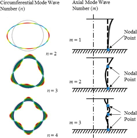
With the reactor internals, the major components, including the reactor vessel (RV), core support barrel (CSB), and upper guide structure (UGS) barrel, are cylindrical. In general, cylindrical structures vibrate in three directions: longitudinal, circumferential, and radial [17]. With the exception of torsional, radial, and longitudinal modes, most vibrational modes of cylindrical structures can be classified as circumferential or bending modes. These vibrational modes can be characterized as (n, m) modes, where n is the circumferential wave number and m is the axial wave number, as shown in Figure 1. Here, MDOFs were selected considering these vibrational modes. The detailed selection criteria are described in following section.

Figure 1. Vibrational modes of the cylindrical structures.

3. Numerical examples and application

3.1. Numerical example 1: a single cylindrical shell in a vacuum

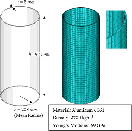
In this section, we describe the MDOF selection method for cylindrical structures by observing the vibrational modes. First, we consider a single cylindrical shell with fixed–free boundary conditions in a vacuum. Figure 2 shows the FE model of the cylindrical shell, which was similar to the CSB in the APR1400. The FE model was constructed using three-dimensional (3D) brick elements (SOLID45 element type in ANSYS), with a total of 12,800 elements (40 elements in the longitudinal direction, 160 elements in the circumferential direction, and two elements in the radial direction), 19,680 nodes, and 59,040 DOFs.

Figure 2. The single cylindrical shell in a vacuum with fixed–free boundary conditions.

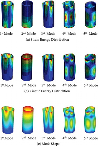
Figure 3 shows the modal energy distribution for the lowest five eigenmodes. The shapes of each eigenmode reflect the energy distribution. By selecting the MDOFs corresponding to the largest deformations of the mode shapes, a large fraction of the modal energy is included in the reduced model. In addition, boundary DOFs are also selected for the MDOFs because the strain energy is concentrated at the boundaries, i.e., where the structures are constrained.

Figure 3. Modal energy distribution of a single cylindrical shell in a vacuum (the lowest five modes).

Figure 4 shows an example of MDOF selection with an axial wave number of 4. With axial vibration, the cylinder vibrates as a beam structure, with nodal lines and maximum deformation, as shown in Figure 4. MDOFs should be selected with maximum deformation lines, avoiding nodal lines. Two MDOF selection methods were compared with the full model, i.e., selecting nodal lines and selecting maximum deformation lines. Figure 5 shows a comparison of the results of the eigenvalue analysis using the two MDOF selection methods. The accuracy was significantly higher when target vibrational modes (m = 4) were selected with maximum deformation. Table 1 lists a comparison of the fraction of the modal energy contained in the elements that were associated with the selected MDOFs. When selecting the MDOFs using the nodal lines, less energy was conserved; in particular, less than 2% of the kinetic energy was retained, indicating that MDOFs should contain the proper modal energies to obtain accurate results.

Figure 4. MDOF selection criterion for the axial direction with m = 4.

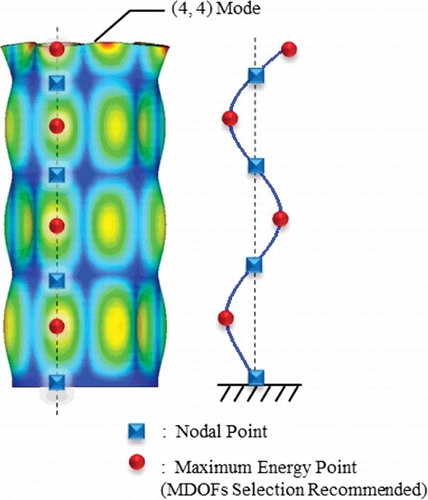
Figure 5. Eigenvalues with various selection criteria for the MDOFs in the axial direction.

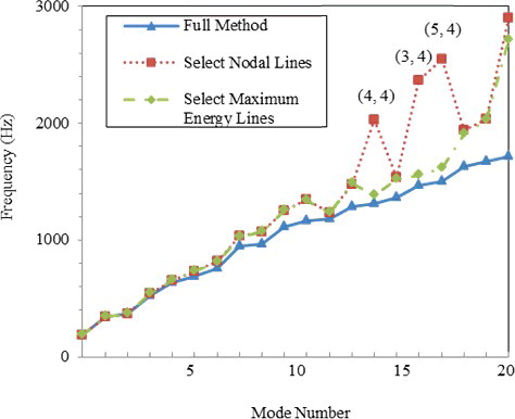
Table 1. Comparison of conserved energies according to the MDOFs selection for a cylindrical shell in a vacuum (target vibrational modes with axial wave number 4).

		Percent of conserved energy in MDOFs (%)
		Maximum deformation lines			Nodal lines
Mode shape (n, m)	Frequency (Hz)	S	K	T	S	K	T
(4, 4)	1306	21.2	35.3	28.2	18.8	1.6	10.2
(3, 4)	1466	14.8	34.8	24.8	8.5	0.9	4.7
(5, 4)	1503	26.6	35.4	31.0	7.6	1.2	4.4

Note: S, K, and T mean strain energy, kinetic energy, and total energy, respectively.

With circumferential vibrational modes, the cylindrical shell deforms along the circumference with axisymmetric vibrational modes. To obtain the mode shapes, MDOFs should be selected uniformly along the circumference; modes with a large circumferential wave number require more MDOFs than smaller wave number modes. Thus, the computational cost should be reduced by selecting MDOFs depending on the frequency range of interest.

Applying these selection criteria, reduced analyses was performed and compared with results from the full model. The 20 lowest order modes were selected for the reduced analysis (i.e., the 20 lowest frequency bending and circumferential modes). Figure 6 shows these corresponding mode shapes, and Table 2 lists the natural frequencies. Several MDOF selection cases were compared to identify the influence of the selection method. Details of the selected MDOFs are shown in Figure 7, and Table 3 summarizes these cases. With manual selection, the locations of the MDOFs along the axis were fixed to 10 lines. These locations were determined by selecting maximum deformation lines of each axial wave number (i.e., m = 1, 2, 3, 4, 5).

Figure 6. The lowest 20 modes of the cylindrical shell in vacuum.

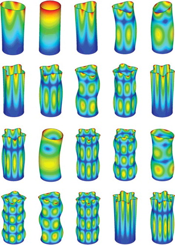
Table 2. The lowest 20 vibrational modes of the cylindrical shell in a vacuum.

Mode shape	Frequency	Mode shape	Frequency
(n, m)	(Hz)	(n, m)	(Hz)
(2, 1)	182.4	(5, 2)	1162
(1, 1)	339.3	(1, 2)	1183
(3, 1)	367.3	(5, 3)	1286
(3, 2)	526.1	(4, 4)	1306
(2, 2)	637.4	(2, 3)	1366
(4, 1)	690.8	(3, 4)	1466
(4, 2)	760.0	(5, 4)	1503
(3, 3)	946.1	(6, 1)	1629
(4, 3)	966.1	(6, 2)	1674
(5, 1)	1113	(4, 5)	1718

Note: In mode shape, n is circumferential wave number and m is axial wave number.

Figure 7. The MDOFs selected for the cylindrical shell in a vacuum (five cases).

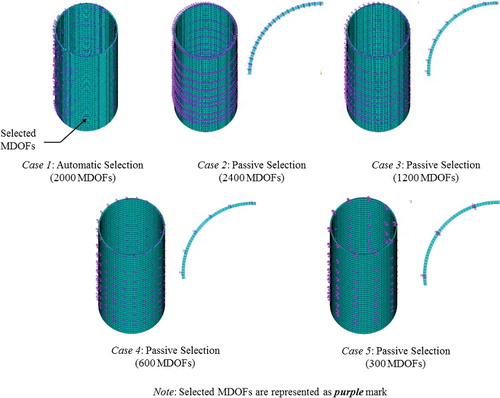
Table 3. Summary of the selected MDOFs for the single cylindrical shell in a vacuum.

Case number	Axial direction	Circumferential direction	Radial direction	Total MDOFs (x, y, z)
1	Automatic selection method in ANSYS			2000
2	Ten lines	Eighty points (4.5 degree intervals)	One point (at outer radius)	2400
3		Forty points (9 degree intervals)		1200
4		Twenty points (18 degree intervals)		600
5		Ten points (36 degree intervals)		300

Figure 8 shows a comparison of the eigenvalues calculated for each case with the results of the full model. We can see that automatic mode selection yielded good results, especially for the lower frequency modes (Case 1). However, some mode shapes exhibited irregular forms because the MDOFs were concentrated on one side of the cylindrical shell, as shown in Figure 9. In contrast to automatic selection, manually selected MDOFs provided accurate results for not only the eigenvalues but also the modal shapes (Case 2). Figure 10 indicates the fraction of conserved modal energy for each eigenmode when selecting the MDOFs with Case 2. As shown in Figure 10, more than 35% of the energy for each mode was retained in the selected MDOFs. In addition, Cases 3, 4, and 5 correspond to MDOF selection with reduction in the circumferential direction. Although the retained modal energy also decreased by reducing the number of MDOFs, the error was not significantly greater than with Case 2. It follows that the accuracy of the results can be preserved by selecting the maximum energy points of each mode. However, in Case 5, significant errors occurred in the circumferential modes with a wave number of 6 because of too few MDOFs describing the deformation points (i.e., 12 DOFs were required). This suggests that the number of MDOFs depends on the modes of interest and that acceptable dynamics can be obtained using optimized MDOFs by selecting the deformation of the parts of the structure in which we are interested.

Figure 8. Comparison of the eigenvalues obtained by the reduced analysis of a cylindrical shell in vacuum.

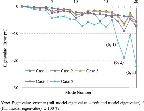
Figure 9. Examples of unexpected mode shapes when using the automatic selection method.

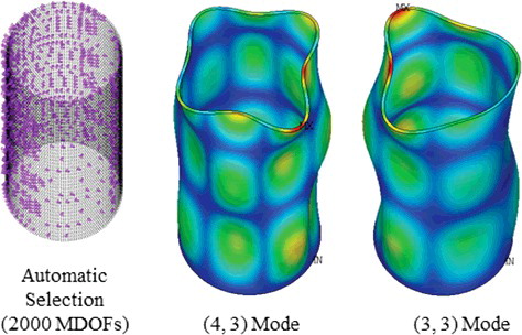
Figure 10. Percentage of modal energies conserved in the selected MDOFs (single cylindrical shell in a vacuum, Case 2).

3.2. Numerical example 2: fluid-filled co-axial cylindrical shells

When structures are submerged in a fluid, FSI effects may become important. FSI should be carefully considered in the vibrational analysis because it can significantly alter the dynamic characteristics of the structures and can lead to coupling between adjacent structures [18]. Considering MDOF selection based on mode shapes, MDOFs for fluid elements can be selected based on the behavior of the structures.

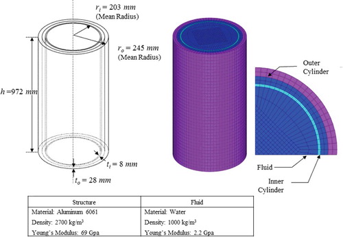
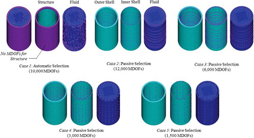
Here, we consider two co-axial cylindrical shells separated by a fluid with fixed-to-free boundary conditions. This geometry is similar to the RV and CSB in the APR1400. Figure 11 shows the FE model for this structure, including the dimensions and material properties. The model was constructed using 3D structural brick elements (SOLID45 element type in ANSYS) and 3D displacement-based fluid elements (FLUID80 element type in ANSYS). The model contained a total of 54,161 elements, with 19,600 solid elements (6400 elements for the inner cylindrical shell and 12,800 elements for the outer cylindrical shell) and 34,481 fluid elements. In total, 62,768 nodes and 188,304 DOFs were noted.

Figure 11. The fluid-filled co-axial cylindrical shells with fixed–free boundary conditions.

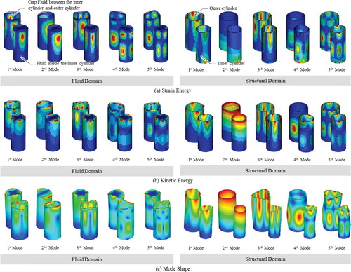
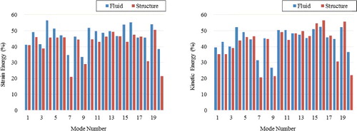
As with the first numerical example (with no fluid), first we identify the modal energy distribution. Figure 12 shows the distribution of modal energy for the lowest five eigenmodes of the fluid-filled co-axial cylindrical shells. In the structural domain, the distribution of modal energies was similar to that of the first numerical example. In the fluid domain, the distribution of modal energies was strongly related to the structural domain because the fluid DOFs were coupled to the structural DOFs at the fluid–structure interface. According to the hydrodynamic effect between the adjacent structures, the modal energy was concentrated in the fluid gap region; e.g., in case of the first eigenmode, 94% of the fluid strain energy and 82% of the fluid kinetic energy were concentrated in the fluid gap region. It follows that the MDOFs should be carefully selected in the fluid gap region to increase accuracy of the reduced model. In addition, we suggest selecting the fluid MDOFs at the fluid–structure interface, because the modal energy of fluid domain was concentrated in the interface elements, as shown in Figure 12. In this manner, the computational cost can be greatly decreased by reducing the total number of MDOFs.

Figure 12. Modal energy distribution of fluid-filled coaxial cylindrical shells (the lowest five modes).

Figure 13 shows the 20 lowest mode shapes, including out-of-phase and in-phase modes, and Table 4 lists the natural frequencies. MDOFs for the fluid region were selected at the interface between the solid and fluid, as shown in Figure 14. In the reduced analysis, several cases were compared. Table 5 lists a summary of the MDOFs selection cases, and the selected MDOFs are presented in Figure 15.

Figure 13. The lowest 20 mode shapes of the fluid-filled co-axial cylindrical shells.

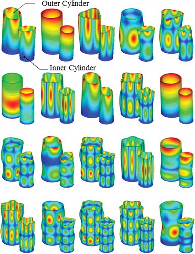
Table 4. The lowest 20 vibrational modes of the fluid-filled co-axial cylindrical shells.

Mode shape	Frequency	Mode shape	Frequency
(n, m)	(Hz)	(n, m)	(Hz)
(2, 1) O	44.74	(3, 3) O	300.4
(1, 1) O	61.63	(2, 3) O	350
(3, 1) O	110.6	(4, 3) O	359.4
(2, 2) O	155.3	(5, 1) O	440.8
(3, 2) O	164.1	(1, 3) O	450.7
(1, 2) O	226.2	(5, 2) O	472.4
(4, 1) O	241.3	(3, 4) O	484.7
(2, 1) I	248.6	(4, 4) O	496.8
(4, 2) O	277.4	(5, 3) O	533.9
(1, 1) I	281.0	(2, 2) I	592.8

Figure 14. MDOF selection considering FSI effects.

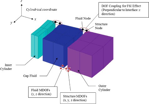
Table 5. Summary of the selected MDOFs for the fluid-filled co-axial cylindrical shells.

Case number	Axial direction	Circumferential direction	Radial direction	Total MDOFs (x, y, z)
1	Automatic selection method in ANSYS			10,000
2	Ten lines	Eighty points (4.5 degree intervals)	Three points (interface of structure and fluid)	12,000
3		Forty points (9 degree intervals)		6000
4		Twenty points (18 degree intervals)		3000
5		Ten points (36 degree intervals)		1500

Figure 15. MDOF selection for the fluid-filled co-axial cylindrical shells (five cases).

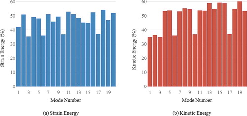
As shown in Figure 16, the calculated eigenvalues using the reduction method were generally in good agreement with the eigenvalues calculated using the full model. It follows that manually selected MDOFs can describe the dynamics of the system, including the FSI by preserving the eigenvalues and mode shapes. However, when MDOFs are automatically selected, eigenvalues of the structures cannot always be calculated because all MDOFs were selected in the fluid region. These results indicate that automatic selection based on the ratio k/m is not appropriate for FSI analysis because the MDOFs of the fluid element were selected preferentially. With manual mode selection, the results show similar trends to those for the single cylindrical shell model with no fluid. At low frequencies, good agreement is expected, with few circumferential MDOFs. However, a larger number of MDOFs is required for higher order circumferential modes. Figure 17 shows the fraction of conserved modal energy for each eigenvalue when selecting MDOFs in Case 2. The modal energies were conserved, not only in the structural region, but also in the fluid region, indicating that the modal energy in the fluid region was preserved effectively by selecting the interfacial DOFs.

Figure 16. Comparison of the eigenvalues obtained from the reduced analysis of fluid-filled co-axial cylindrical shells.

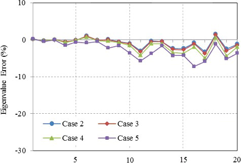
Figure 17. Percentage of modal energies conserved in the selected MDOFs (single cylindrical shell in a vacuum, Case 2).

From these two numerical examples, we can consider the following guidelines to select MDOFs for cylindrical structures:

• For axial modes, MDOFs should be selected near the deformed section and nodal lines should be avoided.

• MDOFs should be properly distributed in the circumferential direction to obtain complete mode shapes of the circumferential modes. We suggest that at least 2n MDOFs be selected for circumferential modes with a wave number n.

• At low frequencies, relatively few MDOFs are required to obtain good agreement with the full model. This may be useful in, for example, seismic analysis, where eigenmodes with natural frequencies of less than 30 Hz are typically significant.

When the fluid elements are included, unnecessary MDOFs may be selected using the automatic selection scheme. In this case, manual selection of MDOFs at the interface of the fluid and structure is effective for obtaining a reduced model that preserves the dynamics of the full model.

4. Application to APR1400 reactor internals

4.1. APR1400 reactor internals

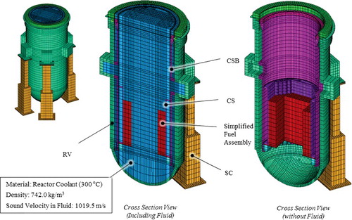
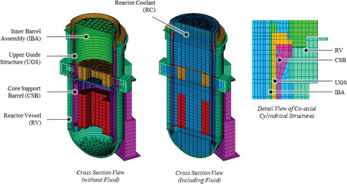
In this section, the model reduction method is applied to the APR1400 internals using the MDOF selection scheme described in the previous section. Here, we focus on the cylindrical structures in the APR1400 internals, and other components are simplified. In the FEA, we validated the FE model using the experimental data for a scaled-down model [1]. The model reduction method was applied to these FE models with various boundary conditions.

4.2. CSB with free end boundary conditions

A single CSB was modeled with free boundary conditions. The FE model was constructed using 44,432 SOLID45 structural elements with 55,416 nodes, as shown in Figure 18. The details of the geometric shape were simplified without changing the principal dynamics. Figure 19 shows the 20 lowest order mode shapes of the CSB components, and the corresponding 20 lowest order eigenvalues are listed in Table 6. Because of the two outlet holes in the center of the CSB, there were slight differences in the eigenvalues, even though they exhibited similar mode shapes, and the same (n, m) modes were present.

Figure 18. An FE model of the CSB component.

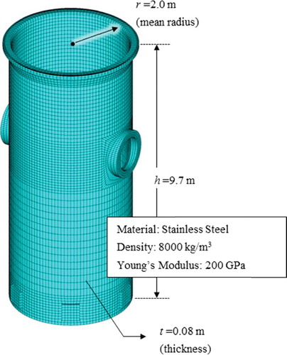
Figure 19. The 20 lowest order mode shapes of the CSB component.

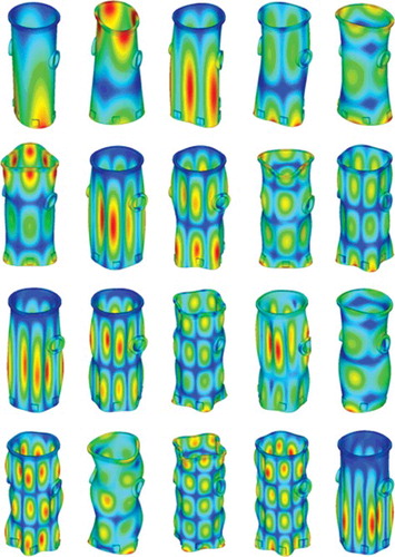
Table 6. The vibrational modes of the CSB component with free boundary conditions.

Mode shape	Frequency	Mode shape	Frequency
(n, m)	(Hz)	(n, m)	(Hz)
(2, 1)	14.70	(3, 3)	70.22
	14.97		71.39
(2, 2)	21.56	(4, 1)	72.59
	21.57		75.52
(3, 1)	39.40	(4, 2)	83.68
	41.59		87.82
(3, 2)	50.76	(3, 4)	101.9
	51.99		103.1
(2, 3)	65.27	(4, 3)	103.0
	68.05		103.1

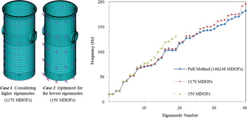
In the reduced model, two different MDOF selection criteria were investigated, whereby the first was optimized for the lower frequency modes and the second for also considering higher frequency eigenmodes. Figure 20 shows a comparison of results for eigenvalues from the full model with results from the reduced model. Although the optimized case provided accurate results at lower frequencies with few MDOFs, the higher frequency eigenmodes were not reproduced. When more MDOFs were included so that higher frequency modes were modeled, good agreement with the full mode was achieved for all eigenmodes.

Figure 20. Results of the reduced analysis of the CSB component.

4.3. CSB assembly clamped to the reactor vessel

Now, we consider a more complex model with different boundary conditions. Figure 21 shows the FE model of the CSB assembly clamped to the RV, which contained a total of 153,948 structural elements and 201,043 nodes, with 603,129 DOFs. In the reduced analysis, we focus on the dominant vibrational modes of the CSB and RV, and other structural modes from the support column and the internal components of the CSB are neglected. Correspondingly, MDOFs were selected with large displacements in the CSB and the RV. Figure 22 shows the selected MDOFs for each structure (there were 1926 MDOFs) considering the lowest 20 mode shapes. A comparison with the model in Section 4.2 shows that the location of the selections changed slightly. This is because the mode shapes were altered by the increased stiffness of the clamped boundaries (top) and the internal structures (bottom). As shown in Figure 22, the same MDOF selection criteria for cylindrical structures were applied to the CSB and the RV. Because the dynamics of the CSB consisted mainly of low-frequency modes, more MDOFs were assigned to the CSB. In addition, boundary DOFs located at the clamped section of the CSB were selected for the MDOFs, considering the strain energy as discussed in Section 3.1. Table 7 lists a summary of the results of the reduced analysis, and Figure 23 shows the mode shapes extracted from the analysis. Figure 24 shows a comparison of the eigenvalues of the lowest 20 modes from the full model with those obtained using the reduced method. The mode shapes and the eigenvalues were in good agreement between the full model and the reduced model.

Figure 21. An FE model of the CSB assembly clamped to the RV in a vacuum.

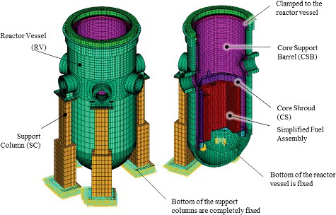
Figure 22. MDOF selection for the clamped CSB assembly in a vacuum.

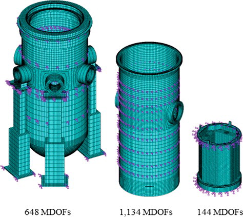
Table 7. The vibrational modes of the CSB assembly clamped to the RV in a vacuum.

	Frequency (Hz)
Mode shape	Full	Reduced	Discrepancy
(n, m)	model	model	(%)
RV (1, 1)	9.771	9.783	−0.2
CSB (1, 1)	15.45	15.48	−0.3
	16.42	16.47	2.6
CSB (2, 1)	39.68	38.64	1.2
	40.03	39.54	−0.1
CSB (3, 1)	45.25	45.3	−0.4
	46.98	47.18	1.8
Second CSB (2, 1)	46.44	45.62	0.4
	47.07	46.88	−2.4
RV (2, 2)	63.93	65.44	−2.4
	64.25	65.8	−1.3
CSB (4, 1)	73.71	74.7	−0.8
	77.21	77.83	−1.2
CSB (3, 2)	79.91	80.83	−1.4
	80.02	81.11	0.1
RV (1, 2)	79.47	79.37	−1.9
CSB (4, 2)	90.41	92.09	−1.1
	94.78	95.86	−0.2

Figure 23. Mode shapes extracted from the reduced analysis of the clamped CSB assembly in a vacuum.

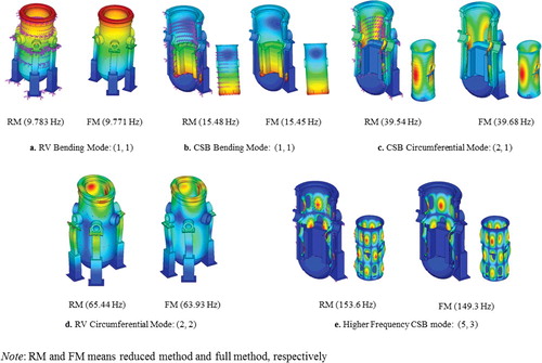
Figure 24. Eigenvalues obtained from the reduced analysis of the clamped CSB assembly in a vacuum.

4.4. Submerged CSB assembly in the reactor vessel

Now, we consider the CSB assembly with FSI effects. Figure 25 shows the FE model in which the CSB assembly was fully submerged in the reactor coolant. The model contained a total of 196,685 elements (81,744 solid and 114,941 fluid elements) and 285,447 nodes (133,522 for the structure and 151,925 for the fluid). 3D displacement-based fluid elements were used, and FSI effects were included from the coupling at the interface with DOFs in the direction perpendicular to the interface.

Figure 25. An FE model of the clamped CSB assembly in fluid.

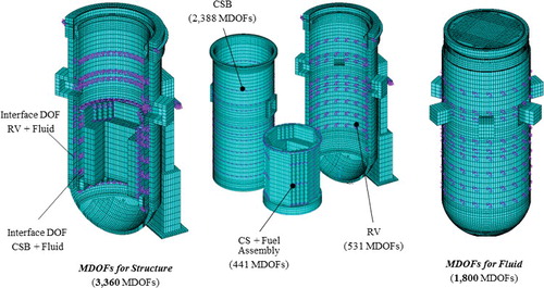
Similar to the numerical example with the fluid-filled co-axial cylindrical shells (see Figure 14), MDOFs were selected at the interface between the solid and fluid regions of the model where the modal energy tended to be concentrated. Considering the lowest 20 mode shapes, a total of 5160 MDOFs (3360 for the solid region and 1800 for the fluid) were distributed in the deformation area. We also considered coupling of the dynamics in the gap fluid between the structures by observing the coupled mode shapes (i.e., in-phase and out-of-phase modes). For this reason, more MDOFs were allocated to the RV compared with the model in the vacuum (see Section 4.3). Figure 26 shows details of the selected MDOFs.

Figure 26. MDOF selection for the clamped CSB assembly in fluid.

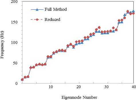
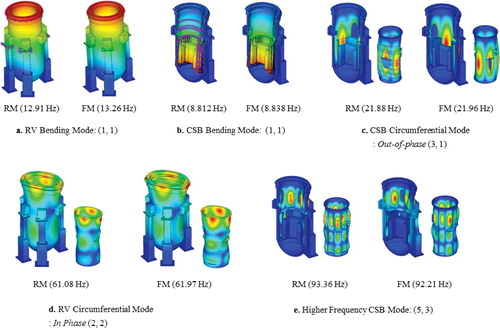
The lowest 40 eigenvalues obtained from the reduced analysis are listed in Table 8, and Figure 27 shows a comparison between the eigenvalues obtained from the reduced analysis and those obtained from the full model. Several selected mode shapes are given in Figure 28. The eigenvalues from the reduced method were in good agreement with the full model, and the mode shapes were also closely matched for each component. Additionally, the reduced model can describe the FSI effects from the coupled mode shapes, e.g., see the RV circumferential mode: in-phase (2, 2) in Figure 28.

Table 8. The vibrational modes of the CSB assembly in the reactor coolant.

	Frequency (Hz)
Mode shape	Full	Reduced	Discrepancy
(n, m)	model	model	(%)
CSB (1, 1)	8.838	8.466	4.2
	9.191	8.715	5.2
RV rotation	13.26	12.91	2.6
	19.25	18.84	2.1
CSB (2, 1)	18.94	18.41	2.8
	19.58	19.07	2.6
CSB (3, 1)	21.96	21.18	3.6
	23.08	22.34	3.2
RV (2, 1)	38.47	36.61	4.8
	40.57	39.12	3.6
CSB (4, 1)	40.06	38.93	2.8
	41.38	39.92	3.5
CSB (3, 2)	41.86	40.08	4.3
	43.58	41.53	4.7
CSB (2, 2)	46.36	43.83	5.5
	47.74	45.89	3.9
CSB (1, 2)	47.59	49.12	−3.2
	54.95	52.21	5.0
CSB (4, 2)	54.27	52.63	3.0
	55.29	52.91	4.3

Note: In the mode shapes, component which shows dominant behavior is written.

Figure 27. Eigenvalues obtained from the reduced analysis of the clamped CSB assembly in fluid.

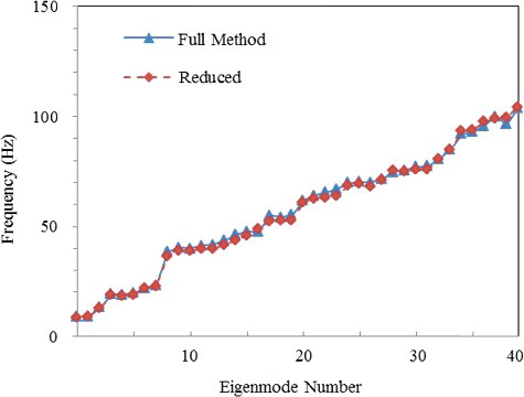
Figure 28. Mode shapes extracted from the reduced analysis of the clamped CSB assembly in fluid.

4.5. Submerged reactor internal assembly

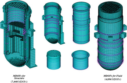
Now, we consider the complete assembled reactor internals with the model reduction method. The UGS and inner barrel assembly (IBA) were additionally assembled to the RV, giving four co-axial cylindrical structures, which may vibrate simultaneously, with coupling via the FSI. Figure 29 shows the FE model of the assembly, including the fluid elements. A total of 562,034 elements were used (184,232 for solid components and 378,072 for the fluid), with 665,019 nodes (242,139 solid nodes and 422,880 fluid nodes).

Figure 29. An FE model of the complete reactor internal assembly.

The MDOF selection criteria described in the previous sections were applied to the reduced analysis. For the complete assembly, many coupled vibrational modes exist because of the FSI effects. For this reason, MDOFs were carefully selected by observing the coupled deformation of each mode. Figure 30 shows the selected MDOFs, focusing on the primary eigenmodes. In total, 11,536 MDOFs were selected. Details of these MDOFs are as follows.

• First, 7440 MDOFs were selected in the structural region.

• For the CSB assembly, sufficient MDOFs were selected considering the overall vibrational modes, including bending modes and circumferential modes. (The number of DOFs decreased from 263,456 to 3081.)

• For the UGS and IBA, MDOFs were selected focusing on the circumferential modes. The number of DOFs for the UGS decreased from 67,473 to 1440, and the number of DOFs for the IBA diminished from 46,083 to 1680.

• For the RV and support columns, MDOFs were selected considering the overall vibrational modes, including bending modes and circumferential modes. (The number of DOFs decreased from 272,310 to 1239.) Fewer MDOFs were chosen for the RV because the eigenvalues of the circumferential modes of the RV were significantly larger than those of the other structures.

• In the fluid region, 4096 MDOFs were selected at the interface of the fluid and structure.

Figure 30. MDOF selection for the complete reactor internal assembly.

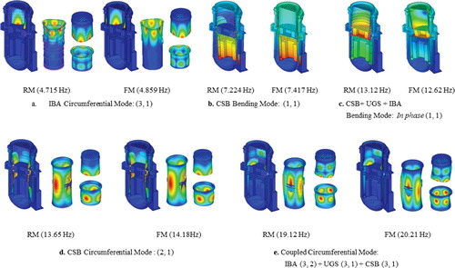
Table 9 lists a comparison of the eigenvalues of the full and reduced models. The eigenvalues obtained using the reduced model were in good agreement with those from the full model. Furthermore, the mode shapes from the reduced method could describe the dynamics of the structure, including the coupled motion due to the FSI effects, as shown in Figure 31.

Table 9. The vibrational modes of the complete reactor internal assembly.

	Frequency (Hz)
Mode shape	Full	Reduced	Discrepancy
(n, m)	model	model	(%)
IBA (3, 1)	4.859	4.715	3.0
IBA (4, 1)	5.758	5.615	2.5
IBA (2, 1)	6.093	5.812	4.6
CSB (1, 1)	7.330	7.125	2.8
	7.417	7.224	2.6
IBA (5, 1)	9.024	8.845	2.0
IBA (1, 1) + UGS (1, 1) OOP	9.834	9.347	5.0
	9.859	9.551	3.1
IBA (1, 1) + UGS (1, 1) + CSB (1, 1) IP	11.79	12.03	−2.0
	12.62	13.12	−4.0
CSB (2, 1)	14.18	13.65	3.7
	14.31	13.89	2.9
CSB (3, 1)	15.65	15.41	1.5
	16.14	15.9	1.5
IBA (3, 2) + UGS (3, 1) + CSB (3, 1)	20.21	19.12	5.4
	20.42	19.55	4.3
IBA (3, 2) + UGS (3, 1) + CSB (3, 2)	25.35	24.12	4.9
	25.62	24.88	2.9
CSB (4, 1)	39.58	37.08	6.3
	39.78	38.14	4.1

Note: (1) In the mode shape, although all structures vibrate simultaneously by dynamic coupling of FSI effect, dominant mode shapes are recorded. (2) In the mode shape, OOP and IP means out-of-phase and in-phase mode, respectively.

Figure 31. Mode shapes extracted from the reduced analysis of the complete reactor internal assembly.

4.6. Comparison of the computational costs

As discussed in the previous sections, the calculated eigenvalues from the reduced model were in good agreement with those from the full model. Here, we discuss the efficiency of the model reduction by considering the time and memory requirements to implement the calculations. Table 10 lists the required computational costs for performing the eigenvalue analyses (i.e., extracting 100 eigenvalues). All analyses were carried out using the same computing environment, i.e., a machine with an Intel Xeon X5660 2.8-GHz processor with six cores. The overall computational costs decreased significantly when using the model reduction method. In particular, with Model 1 (i.e., CSB with free end boundary conditi- ons), the time for the calculation decreased from 60 to 2 s, and the memory requirements decreased from 885,589 to 1901 kB. The reduced analysis was also effective in reducing the computational cost of the large-scale Model 4 (i.e., submerged reactor internal assembly), although the reduction in computational expense was less marked than with the small-scale model.

Table 10. Computation costs for performing the eigenvalue analysis of the reactor internals: comparison of full model and reduced model.

	Number of DOFs		Computation time (second)		Required memory (Kbytes)
Model type	Full model	Reduced model	Full model	Reduced model	Full model	Reduced model
Model 1	166,248	1170	60	2	885,590	1901
Model 2	603,129	1926	123	7	2,188,672	49,677
Model 3	856,341	5160	2427	87	3,368,281	332,400
Model 4	1,995,057	11,536	10,703	1143	8,050,807	2,913,207

Note: “Model 1–4” denotes the CSB with free end boundary conditions, CSB assembly clamped to the RV, submerged CSB assembly in the RV, and submerged reactor internal assembly, respectively.

5. Conclusion

We have described the application of a model reduction method to the internal components of the APR1400 to reduce the computational expense of FEM vibrational analyses. To improve accuracy and avoid unnecessary MDOFs, we manually selected the MDOFs with the large modal energies by observing the shapes of the eigenmodes.

As part of the selection scheme, we analyzed the vibrational characteristics of the main components of the internals of the reactor, which were cylindrical. Focusing on the vibrational modes of the cylindrical structure, the MDOF selection criteria were for large circumferential and axial motion. With FSI problem, MDOFs for the fluid were selected based on the mode shapes of the interacting structures. The DOFs at the interface between the structure and the fluid were selected to describe the FSI. To assess these selection criteria, two numerical examples with simple cylindrical shells were investigated with and without the fluid. We examined several cases to identify the efficiency and the accuracy of the selection criteria based on the vibrational modes. This model reduction method was found to provide eigenvalues and mode shapes that were in good agreement with the full model which also shows that a large fraction of the modal energy was conserved in the selected MDOFs. When the FSI effect was included, it also provided reasonable results, representing changes in the dynamics due to the coupling caused by the fluid.

We applied these selection criteria to an FE model of the internal structure of an APR1400 with several boundaries and assembly variations. The reduced method was found to provide not only accurate results in terms of the eigenvalues and the mode shapes, but also significant reductions in computational expense by reducing the number of DOFs. For example, in the case of the submerged reactor internal assembly, the overall eigenvalues for each mode were in good agreement with the full model (to within ±7%), and the number of DOFs used in the analysis decreased from 1,995,057 to 11,536. In addition, the time required to calculate the eigenvalues decreased from 10,703 to 1143 s.

The method described here requires some input to analyze the mode shapes prior to MDOFs selection; however, it provides accurate results and the total number of MDOFs can be reduced significantly, depending on the desired frequency range. There is significant scope for further work in the application of these methods to the analysis of the reactor internals, including seismic analysis. As part of future work, we plan to extend this approach to the dynamic analysis of reactor internals and develop MDOFs selection criteria for related problems.

Acknowledgements

The support of Korea Institute of Nuclear Safety (KINS), which has designated this research as a specialization project by Yonsei University, is gratefully acknowledged. Acknowledgement is also given to the project “Modal test with scaled-down model for identifying dynamic characteristics of main components in reactor/Analysis model construction for evaluating validity of seismic design”.

Disclosure statement

No potential conflict of interest was reported by the authors.

References

- Park JB, Choi Y, Lee SJ, Park NC, Park KS, Park YP, Park CI. Modal characteristic analysis of the APR1400 nuclear reactor internals for seismic analysis. Nucl Eng Technol. 2014;46:689–698.
- Choi Y, Park J, Park NC, Park YP, Park KS, Jeong KH. Application of seismic analysis methodology to small modular integral reactor internals. J Nucl Sci Technol. 2015;52:228–240.
- Law M, Phani AS, Altintas Y. Position-dependent multibody dynamic modeling of machine tools based on improved reduced order models. J Manufacturing Sci Eng. 2013;135:021008.
- Arnoux A, Batou A, Soize C, Gagliardini L. Stochastic reduced order computational model of structures having numerous local elastic modes in low frequency dynamics. J Sound Vibration. 2013;332:3667–3680.
- Flodén O, Persson K, Sandberg G. Reduction methods for the dynamic analysis of substructure models of lightweight building structures. Comput Struct. 2014;138:49–61.
- Ramsden JN, Stoker JR. Mass condensation: a semi-automatic method for reducing the size of vibration problems. Int J Numer Methods Eng. 1969;1:333–349.
- Downs B. Accurate reduction of stiffness and mass matrices for vibration analysis and a rationale for selecting master degrees of freedom. J Mechanical Des. 1980;102:412–416.
- Popplewell N, Bertels AWM, Arya B. A critical appraisal of the elimination technique. J Sound Vibration. 1973;31:213–233.
- Henshell RD, Ong JH. Automatic masters for eigenvalue economization. Earthquake Eng Struct Dyn. 1974;3:375–383.
- Matta KW. Selection of degrees of freedom for dynamic analysis. J Press Vessel Technol. 1987;109:65–69.
- Kim KO, Choi YJ. Energy method for selection of degrees of freedom in condensation. AIAA J. 2000;38:1253–1259.
- Cho M, Kim H. Element-based node selection method for reduction of eigenvalue problems. AIAA J. 2004; 42:1677–1684.
- Kim H, Cho M. Study on the system reduction under the condition of dynamic load. J Mechanical Sci Technol. 2013;27:113–124.
- Guyan RJ. Reduction of stiffness and mass matrices. AIAA J. 1965;3:380.
- Chen HC, Taylor RL. Vibration analysis of fluid-solid systems using a finite element displacement formulation. Int J Numer Methods Eng. 1990;29:683–698.
- Meirovitch L. Elements of vibration analysis. 2nd ed. New York (NY): McGraw-Hill Book Company; 1986.
- Markuš Š. The mechanics of vibrations of cylindrical shells (Vol. 17). Amsterdam: Elsevier Science Ltd.; 1988.
- Fritz RJ. The effect of liquids on the dynamic motions of immersed solids. J Manufacturing Sci Eng. 1972;94:167–173.