Development of natural circulation analysis methods for a sodium cooled fast reactor

Abstract

A natural circulation evaluation methodology has been developed to insure safety of a sodium cooled fast reactor (SFR) of 1500 MWe adopting a natural circulation decay heat removal system (NC-DHRS). The methodology consists of a one-dimensional safety analysis which can be applied to safety evaluation for SFR licensing taking into account the temperature flattening effect due to buoyancy force in the core, and a three-dimensional fluid flow analysis which can evaluate thermal-hydraulics for local convection and thermal stratification in the primary system and DHRSs. The one-dimensional safety analysis method and the three-dimensional fluid flow analysis method have been validated using the test results of a water test apparatus and a sodium test loop for some typical transient events selected from the design basis events of the SFR. Finally, it has been confirmed that a good agreement between the test results and analysis results has been obtained, and reliability of each method has been demonstrated.

Keywords:

• fast reactor
• passive decay heat removal
• natural circulation
• CFD
• thermal hydraulics

1. Introduction

Based on the study results of the past, a natural circulation evaluation methodology has been developed to insure safety of a sodium cooled fast reactor (SFR) of 1500 MWe being designed in Japan [1] for which a natural circulation decay heat removal system (NC-DHRS) has been adopted. The NC-DHRS is automatically activated at all the reactor trip events including not only at an event of loss of off-site power (symmetrical event) but also at asymmetrical events of loop operation of the SFR.

One-dimensional flow network analysis models have widely been used for safety analyses of SFR plants because of simplicity and easiness of handling, and one has been applied to the safety analysis for licensing of the Japanese prototype SFR, MONJU [2]. Therefore the one-dimensional flow network model is expected to be applied to future licensing of the SFR with NC-DHRS, but applicability of existing one-dimensional flow network analysis models has not been sufficiently confirmed for the SFR. Compared with a forced circulation system the core temperature is higher with a natural circulation system because the primary flow rate is smaller. The flow rate of the NC-DHRS strongly depends on the temperature distribution while the primary flow rate of the forced circulation system is determined mainly by the number of rotation of the primary pump driven by a pony motor. Thus the temperature distribution in the primary system, the large sodium plena and the large diameter piping has to be simulated more accurately than for the forced circulation system. On the other hand, the NC-DHRS has a very beneficial characteristic called “temperature flattening effect” [3] which causes a significant decrease of the core hot spot temperature accompanied by the inter- and intra-subassembly flow redistributions and radial heat transfer with the inter-wrapper gap flow (IWF) due to buoyancy, and thus high thermal conductivity of sodium and the temperature flattening effect should be taken into the future safety analyses for the SFR.

In this study a safety analysis method based on the one-dimensional flow network analysis model has been developed to evaluate the core hot spot temperature taking into account the temperature flattening effect in the core and to simulate the temperature distribution in the primary system more accurately. A three-dimensional fluid flow analysis method, which can simulate precisely thermal-hydraulics such as thermal stratifications and local convections in the primary system together with the temperature flattening effect, has also been developed to support the one-dimensional safety analyses for future licensing of the SFR. The three-dimensional fluid flow analysis method can also evaluate the scale effect due to the difference of dimensions between the SFR and the validation test, because it can exactly deal with the geometry and has the turbulent models as well. The one-dimensional safety analysis method is planned to be incorporated into statistical safety evaluation [2,4] because of its fast running time. Moreover, both the one-dimensional safety analysis method and three-dimensional fluid flow analysis method have been validated using the test results of a 1/10-scale water test [5] and a 1/7-scale sodium test [6] for five typical transient events selected from the design basis events (DBE) of the SFR. In order to demonstrate further reliability of both methods, blind analyses have been carried out by using some water test data [7] and it has been confirmed that both methods show a good agreement with the test data as well as the validation analyses.

This paper describes the development of the one-dimensional safety analysis and three-dimensional fluid flow analysis methods for the SFR and their validation results. The overall description of the related studies will be given as a separate paper [8].

2. Natural circulation decay heat removal system

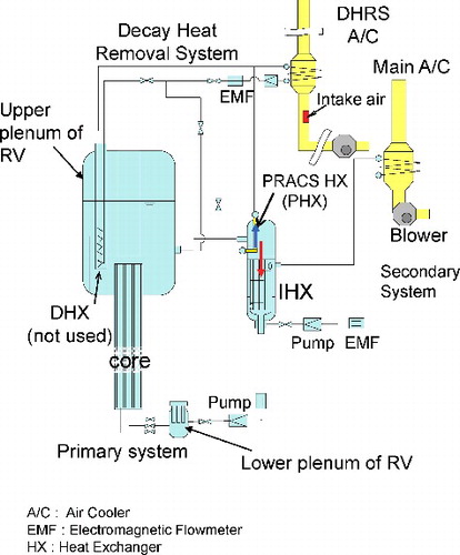
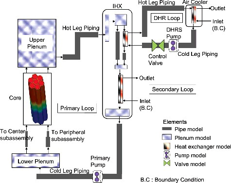
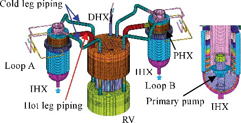
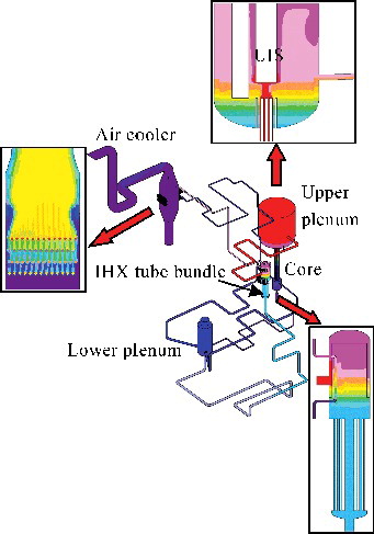
The SFR consists of two main heat transport systems [1] as shown in Figure 1. Each primary loop consists of a hot-leg pipe, a pair of cold-leg pipes and an intermediate heat exchanger (IHX) into which a primary pump is installed. The DHRS for the SFR consists of one unit of direct reactor auxiliary cooling system (DRACS) and two units of primary reactor auxiliary cooling system (PRACS). The DRACS has a heat exchanger (DHX) installed in the upper plenum of the reactor vessel (RV). Each PRACS has a heat exchanger (PHX) installed in the upper plenum of the IHX. These safety systems can be operated under passive natural circulation without active operation of pumps and blowers. The system only requires DC power supplied by battery backup systems to operate the dampers of the air coolers [9].

Figure 1. Schematic of the SFR heat transport systems.

3. Development of computational methods

3.1. One-dimensional safety analysis method

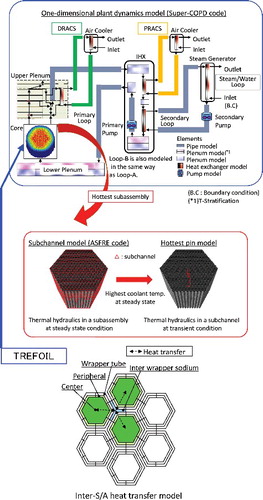
The one-dimensional safety analysis method has been developed to evaluate the core hot spot temperature taking into account the temperature flattening effect in the core and to simulate the temperature distribution in the primary system accurately by incorporating the whole core thermal-hydraulic analysis code, TREFOIL, and a newly developed hottest fuel pin model in the one-dimensional plant dynamics analysis code, Super-COPD [10,13], as shown in Figure 2, and by improving the one-dimensional model for the large sodium plena and large diameter piping in the primary system. TREFOIL [11] can evaluate the temperature flattening effect taking into account the inter-subassembly flow redistribution and radial heat transfer with IWF in the core. With the hottest fuel pin model one can evaluate the temperature flattening effect taking into account the intra-subassembly flow redistribution and energy exchanges between the hottest sub-channel and average sub-channel in the fuel subassemblies. The mixing coefficient for the energy exchanges caused by the cross flows due to the wrapping wires around the fuel pins has been obtained through a survey analysis by use of the sub-channel analysis code ASFRE [12]. Super-COPD is an improved version of the plant dynamics analysis code applied to the safety analysis for licensing of the Japanese prototype SFR, MONJU [10,13] and its one-dimensional flow network model is composed of the flow elements, mixture elements and heat exchanger elements with various functions. As an example, the basic equations of the flow elements and heat exchanger elements are shown below. When a flow network is composed of M pressure nodes and N flow channels, the mass and momentum conservation equations of the flow elements are given in Equations (1)(1) $$\sum _{j\in Ii}{a}_{i,j}{G}_j=S_i(i=1,...,M),$$(1) and (2(2) $$\begin{array}{ccc}\hfill \sum _{i\in Jj}-a_{i,j}{P}_i& =& F_j{G_j}^{{\alpha }_i}-\Delta H_j-E_j+V_j\left|G_j\right|G_j\hfill \\ & & +L_j\left(\frac{d{G}_j}{dt}\right)(j=1,...,N),\hfill \end{array}$$(2) ), (1) $$\sum _{j\in Ii}{a}_{i,j}{G}_j=S_i(i=1,...,M),$$(1) (2) $$\begin{array}{ccc}\hfill \sum _{i\in Jj}-a_{i,j}{P}_i& =& F_j{G_j}^{{\alpha }_i}-\Delta H_j-E_j+V_j\left|G_j\right|G_j\hfill \\ & & +L_j\left(\frac{d{G}_j}{dt}\right)(j=1,...,N),\hfill \end{array}$$(2) where I_i is the set of flow channels connected to a pressure node i and J_j is the set of pressure nodes connected to a flow channel j. The coefficient a_{i, j} is +1 for inlet and −1 for outlet at the pressure node i and flow channel j. The variables G, S, P, F, α, ΔH, E, V and L are the mass flow rate, source of mass, pressure, pressure loss normalized to the initial flow rate, exponent of pressure loss, buoyancy induced pressure (natural circulation force), driving pressure by circulation pumps, additional pressure loss due to valves normalized to the initial flow rate, and the fluid inertia, respectively.

Figure 2. Outline of one-dimensional safety analysis model.

The conservation of energy in the heat exchanger elements is expressed by the following partial differential equations (3(3) $$\begin{array}{ccc}\hfill C_p{M}_p\frac{\partial }{\partial t}{T}_p& =& -C_p{G}_p\frac{\partial }{\partial Z}{T}_p-U_1{A}_1(T_p-T_t)\hfill \\ & & -U_3{A}_3(T_p-T_{\mathrm{sh}}),\hfill \end{array}$$(3) )–(6) in time t and one spatial dimension Z,

for the outer tube coolant: (3) $$\begin{array}{ccc}\hfill C_p{M}_p\frac{\partial }{\partial t}{T}_p& =& -C_p{G}_p\frac{\partial }{\partial Z}{T}_p-U_1{A}_1(T_p-T_t)\hfill \\ & & -U_3{A}_3(T_p-T_{\mathrm{sh}}),\hfill \end{array}$$(3) for the tube: (4) $$C_{\mathrm{t}}{M}_t\frac{\partial }{\partial t}{T}_t=U_1{A}_1(T_p-T_t)-U_2{A}_2(T_t-T_s),$$(4) for the inner tube coolant: (5) $$C_{\mathrm{s}}{M}_s\frac{\partial }{\partial t}{T}_s=C_s{G}_s\frac{\partial }{\partial Z}{T}_s+U_2{A}_2(T_t-T_s),$$(5) for the shell: (6) $$\begin{array}{ccc}\hfill C_{\mathrm{sh}}{M}_{\mathrm{sh}}\frac{\partial }{\partial t}{T}_{\mathrm{sh}}& =& U_3{A}_3(T_p-T_{\mathrm{sh}})-U_4{A}_4(T_{\mathrm{sh}}-T_{\mathrm{air}})\hfill \\ & & -U_5{A}_5(T_{\mathrm{sh}}-T_{\mathrm{EX}}),\hfill \end{array}$$(6) where the variables C, M, U and A are the specific heat, mass per unit length, heat transfer coefficient and heat transfer area per unit length, respectively, and the subscripts p, t, s, sh, air and EX indicate the outer tube coolant, tube, inner tube coolant, shell, atmospheric air and the other heat transfer substances, respectively, and the subscripts 1, 2, 3, 4 and 5 indicate heat transfers between the outer tube coolant and tube, between the tube and inner tube coolant, between the outer tube coolant and the shell, between the shell and the atmospheric air, and between the atmospheric air and the other heat transfer substances, respectively.

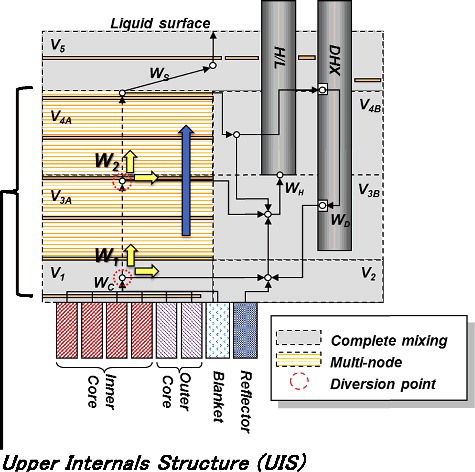
Furthermore, the one-dimensional safety analysis method has been improved to reflect the validation analysis results using the 1/10-scale water test [5] and the 1/7-scale sodium loop test [6]. Improvement has been made mainly for the large plena, such as the reactor upper plenum and large diameter primary pipes where three-dimensional complex flows due to buoyancy are expected. The improved reactor upper plenum analysis model is shown in Figure 3 as an example of the improvement. To simulate the upper plenum thermal-hydraulics in the process of transition from the forced circulation to the natural circulation, the volume division of the upper plenum has been elaborated. The upper plenum is divided into the inner and outer regions of the upper internals structure (UIS) in the radial direction and divided by levels of the hot-leg intake, DRACS (DHX) intake and the lowest baffle plates of the UIS such as (V1, V3A, V4A) and (V1, V2, V3B, V4B, V5) in the vertical direction. The upper core volumes, V3A, V4A, are further divided into the one-dimensional meshes in the flow direction, and the other volumes are treated as complete mixing regions. The flow rate ratio, W₁/W_c, is given by a function of the Richardson number (Ri) calculated by the temperature difference between the V1 and V2, and core outlet velocity. The function related to the Ri number has been determined by the 1/10-scale water test analyses.

Figure 3. Improved reactor upper plenum analysis model.

3.2. Three-dimensional fluid flow analysis method

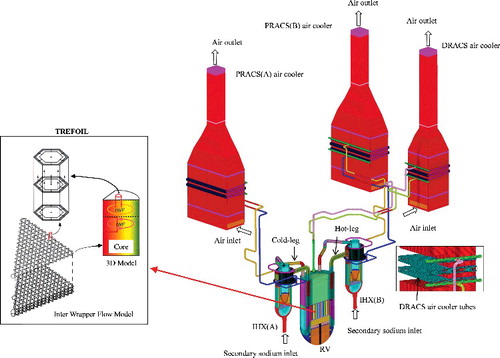
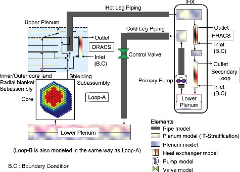
As a backup of the one-dimensional safety analysis a three-dimensional fluid flow analysis method has been developed to analyze thermal-hydraulic phenomena in the primary system and DHRS under decay heat removal conditions for the SFR by inserting TREFOIL and a primary pump coast-down calculation routine into the computational fluid dynamic analysis code “STAR-CD (Vr4.14)” [14] as shown in Figure 4. Coupling TREFOIL and STAR-CD, the flow rates and inlet temperatures of subassemblies are transferred from STAR-CD to TREFOIL and the pressure losses and temperature distributions in the subassemblies are transferred from TREFOIL to STAR-CD internally. The temperature distributions in the subassemblies are used for buoyancy calculations in STAR-CD. The power generation rate in the core, inlet air temperature of the air coolers in the PRACSs and DRACS and secondary side inlet temperature of IHX are given as the boundary conditions for the three-dimensional fluid flow analysis during the reactor trip transient.

Figure 4. Structure of three-dimensional method.

The RNG (re-normalization group) k–ϵ turbulent model [15,16] is applied to the three-dimensional fluid flow analysis as an option in STAR-CD to avoid overestimation of turbulent kinetic energy at the impingement and separation regions in the flow. And a second-order advection scheme named MARS (monotone advection and reconstruction scheme) [17] is also selected as an option in STAR-CD to reduce the numerical diffusion and wiggles simultaneously. The basic equations of the RNG k–ϵ turbulent model for turbulent kinetic energy k and its dissipation rate ϵ are as follows: (7) $$\begin{array}{c}{\displaystyle \frac{\partial }{\partial t}\left(\rho k\right)+\frac{\partial }{\partial x_j}\left({\displaystyle \rho u_{j}k-\left({\displaystyle \mu +\frac{{\mu }_t}{{\sigma }_k}}\right)\frac{\partial k}{\partial x_j}}\right)}\hfill \\ {\displaystyle =P+P_B-\rho ϵ-\frac{2}{3}\left({\displaystyle {\mu }_t\frac{\partial u_i}{\partial x_i}+\rho k}\right)\frac{\partial u_i}{\partial x_i},}\hfill \end{array}$$(7) (8) $$\begin{array}{c}{\displaystyle \frac{\partial }{\partial t}\left(\rho ϵ\right)+\frac{\partial }{\partial x_j}\left({\displaystyle \rho u_jϵ-\left({\displaystyle \mu +\frac{{\mu }_t}{{\sigma }_{ϵ}}}\right)\frac{\partial ϵ}{\partial x_j}}\right)}\hfill \\ {\displaystyle =C_{ϵ1}\frac{ϵ}{k}\left[{\displaystyle P-\frac{2}{3}\left({\displaystyle {\mu }_t\frac{\partial u_i}{\partial x_i}+\rho k}\right)\frac{\partial u_i}{\partial x_i}}\right]}\hfill \\ {\displaystyle +C_{ϵ3}\frac{ϵ}{k}{P}_B-C_{ϵ2}\rho \frac{{ϵ}^2}{k}+C_{ϵ4}\rho ϵ\frac{\partial u_i}{\partial x_i}}\hfill \\ {\displaystyle -\frac{C_{\mu }{\eta }^3\left({\displaystyle 1-\frac{\eta }{{\eta }_0}}\right)}{1+\beta {\eta }^3}\frac{\rho {ϵ}^2}{k},}\hfill \end{array}$$(8) where (9) $${\displaystyle {\mu }_t=\frac{C_{\mu }\rho k^2}{ϵ},}$$(9) (10) $${\displaystyle P={\mu }_t\frac{\partial u_i}{\partial x_j}\left({\displaystyle \frac{\partial u_i}{\partial x_j}+\frac{\partial u_j}{\partial x_i}}\right)={\mu }_t\frac{\partial u_i}{\partial x_j}{S}_{ij},}$$(10) (11) $${\displaystyle P_B=-{\mu }_t\frac{g_i}{{\sigma }_h}\frac{1}{\rho }\frac{\partial \rho }{\partial x_i},}$$(11) (12) $${\displaystyle \eta =\frac{Sk}{ϵ},}$$(12) (13) $$S={\left({\displaystyle \frac{1}{2}{S}_{ij}{S}_{ij}}\right)}^{1/2},$$(13) and μ_t is turbulent eddy viscosity, P and P_B are productions of the turbulent kinetic energy due to strain rate S_ij and buoyancy, respectively. The constants in the above equations are as follows: (14) $$\begin{array}{c}{C}_{\mu }=0.085,{\sigma }_k={\sigma }_{ϵ}=0.719,{\sigma }_h=0.9,\hfill \\ C_{ϵ1}=1.42,C_{ϵ2}=1.68,C_{ϵ3}=1.42(P_B\ge 0)\hfill \\ \mathrm{or}0.0,C_{ϵ4}=-0.387,{\eta }_0=4.38,\beta =0.012.\hfill \end{array}$$(14)

The wall friction and heat transfer are calculated by the standard logarithmic law on the wall as follows: (15) $${\tau }_w=\rho u_{\tau }^2,$$(15) (16) $${\displaystyle q_w=\frac{\rho C_p{u}_{\tau }}{P_{rt}}(T_f-T_w),}$$(16) (17) $${\displaystyle \frac{U}{u_{\tau }}=\frac{1}{\kappa }log\left(E{y}^{+}\right)=\frac{1}{\kappa }log\left({\displaystyle E\frac{u_{\tau }\delta }{\nu }}\right),}$$(17) where τ_w, q_w, T_w and u_τ are the tangential stress, heat flux, temperature and slip velocity on the wall; U and T_f are the tangential velocity and temperature of the fluid adjacent to the wall; C_p, ν and ρ are the specific heat, kinematic viscosity and density of the fluid; κ is the Karman constant (= 0.4) and E (= 9.0) is the empirical constant for smooth walls; δ is the distance between the center of the adjacent fluid cell and wall; and Pr_t is the turbulent Prandtl number (≈ 0.9).

4. Validation analyses

4.1. Outline of water and sodium tests

4.1.1. Water test apparatus

Water tests were performed using a 1/10-scale model which simulates the primary system of the SFR at Central Research Institute of Electric Power Industry [5]. The upper plenum of the RV, upper plenum of the IHXs including the heat transfer tubes for PRACS and hot- and cold-leg piping are made of acrylic material to be able to observe thermal-hydraulic phenomena directly. The core region is divided into three zones, i.e. the inner core, outer core and radial blanket. Each zone consists of a number of vertical channels with electric heaters simulating heat generation of the SFR subassemblies. The temperature rise from the core inlet to the outlet is set as 9.3 °C corresponding to 155 °C of the SFR at the full power. The rated power of the apparatus is about 120 kW enabling to simulate transient phenomena from forced circulation to natural circulation. The core power of the natural circulation mode is about 17 kW according to the similarity rule.

The similarity rule of the natural circulation tests has been discussed in a previous study for a top-entry type SFR [5], indicating that there are three major dimensionless parameters to be considered: the Euler number (Eu), modified Boussinesq number (Bo) and modified Grashof number (Gr). The Eu number stands for the ratio of pressure loss to inertial force, which is equivalent to half the value of the pressure loss coefficient in a continuous flow conduit, and the summation of Eu along the primary system is equal to the Ri that stands for the ratio of natural circulation force to inertial force. The Bo^1/2 and Gr^1/2 numbers are equivalent to the Peclet number (Pe) and the Re number in case of forced convection, respectively, and Bo^1/2 and Gr^1/2 are convenient for identifying the natural circulation test conditions because the representative flow velocity depends on the heating power. It is ideal to carry out the scale model test based on the similarity rule matching the above dimensionless numbers to those of the SFR. However, it is practically impossible to match the three dimensionless numbers at the same time. Therefore, the water test has been performed with matching Eu while Bo^1/2 of the water test is set at the same order as that of the SFR (by about factor three larger than that of the SFR). Under this test condition, though Gr^1/2 equivalent to Re is reduced to about 1/350 of the SFR, its absolute value is as high as several thousands in the primary piping. Therefore, the flows during the water test are likely to stay in turbulent states in major parts of the apparatus.

4.1.2. Sodium test apparatus

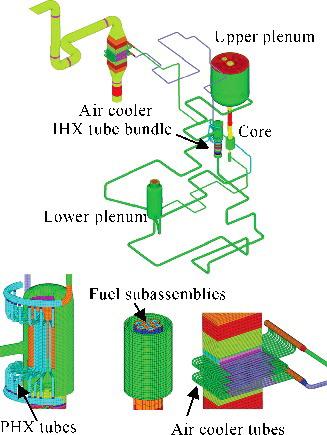
Sodium tests were conducted using Plant Dynamics Test Loop (PLANDTL) [6] of Japan Atomic Energy Agency O-arai Research and Development Center. The objectives of the sodium tests are to evaluate the heat transfer characteristics of the PHX under natural circulation condition and to confirm transition behavior from steady forced circulation state to natural circulation state for an integrated system consisting of the primary sodium system, secondary sodium system of the PRACS and tertiary air cooling system. The IHX partially simulating the PHX was manufactured and installed at PLANDTL as shown in Figure 5. The primary system consists of the core with seven mock-up fuel subassemblies, an electromagnetic pump, an IHX, an RV simulating the upper plenum, lower plenum, and pipes connecting these components. The secondary system consists of an electromagnetic pump, a hot-leg pipe and a cold-leg pipe, and an air cooler. The DHRS consists of a PHX installed in the upper plenum of the IHX, an electromagnetic pump, a hot-leg pipe and a cold-leg pipe, an air cooler with a blower, and an air dumper in the inlet duct and outlet duct. The geometry of the primary system of PLANDTL is not an exact mock-up of the SFR design as compared with that of the 1/10-scale water test apparatus; however, sodium tests can be conducted under the equivalent Ri condition for the DHRS of the SFR. Heat removal capability of the PRACS has been chosen as 100 kW taking into account the Ri similarity and the model scale of nearly 1/7 of the SFR. On the other hand, the PHX consists of straight heat transfer tubes arranged along the outer shroud of the upper plenum of the IHX so as to simulate heat transfer on the outer walls of the tubes of the SFR. Under high flow rate conditions of the rated power operation the primary coolant flows down uniformly through the annular region between the outer shroud and the inner shroud with a relatively low pressure loss. Under low flow rate conditions of the natural circulation regime the coolant flows down around the PHX heat transfer tubes locally due to the buoyancy effect. It was required for the sodium test to employ heat transfer tubes of the same size as the actual plant in order to verify the heat transfer characteristics of the PHX under the SFR equivalent Pe condition.

Figure 5. Schematics of plant dynamics test loop (PLANDTL).

4.2. Validation of one-dimensional safety analysis method

4.2.1. 1/10-scale water test analysis

The purpose of this study is to develop a safety analysis method that can be applied to the SFR. Validation has been performed for the primary flow rate, inlet temperature and outlet temperature of the RV which interact mutually under the natural circulation regime. The discrepancies of the primary flow rate and RV inlet temperature between the validation analyses and test results are reflected to the modeling errors of the one-dimensional safety analysis method for the SFR by applying the similarity rule. And then the modeling error for the core outlet temperature is quantified by TREFOIL using the boundary conditions in consideration of their errors. The overall description of the statistical core hot spot evaluation will be given as a separate paper [17]. Therefore the evaluation targets are the primary flow rate, RV inlet temperature and outlet temperature. Figure 6 shows the one-dimensional flow network model for the 1/10-scale water test. In order to apply the validated one-dimensional safety analysis method to SFR evaluation, each node of the analytical model has to be matched to that of SFR. Prior analyses have been performed to determine the model constants in the functions of the local Ri number for the RV upper plenum and other components. This process for the RV upper plenum model is shown below as a typical example. The temperature transients at each region of the RV upper plenum model are simulated with several variable sets of the model constants, and these constants are determined by optimization analyses. The optimization analyses are performed minimizing the sum of the squares of the differences and the negative correlation between the measured data and the analytical values for the duration of 10,000 seconds employing the genetic algorithm [18]. The negative correlation means that there is an opposite trend between the measured data and analytical values.

Figure 6. One-dimensional modeling for water test analyses.

Validation analyses have been carried out using the model constants determined solely by representative 13 water tests chosen from the following five categories of the DBE of the SFR, (1) loss of off-site power, (2) sodium leakage in the secondary loop, (3) sodium leakage in the secondary-side-of-DRACS, (4) sodium leakage in the secondary side of PRACS, and (5) one pump stick in the primary loop. The summary of the validation analysis cases for these water tests is shown in Table 1. The boundary conditions of the analyses such as the core power decrease, primary pump coast-down curves, secondary side inlet flow rates and temperatures of the IHX, DHX and PHX have been given to the one-dimensional flow network model as input data. The common analysis parameters have been used for all of the tests. Confirmation of agreement has been obtained as a result of the validation analyses with similar degrees of agreement for almost all cases. The following two events have been picked up in this paper as typical cases.

Table 1. Summary of the validation analysis cases for water tests.

No.	Transient events	Notes
1	Loss of off-site power	Reference
2		Flow coast-down time is shorter than the reference for 50 seconds.
3		Flow coast-down time is longer than the reference for 50 seconds.
4		Startup times DHRS is earlier than the reference for 100 seconds.
5		Startup times DHRS is later than the reference for 100 seconds.
6		Startup times DHRS is later than the reference for 300 seconds.
7	Sodium leakage in the secondary loop	Failure loop B
8		Failure loop A
9	Sodium leakage in the secondary side of PRACS	Reference (failure loop A)
10		Reference + one damper fails in PRACS B + DRACS forced circulation
11	Sodium leakage in the secondary side of DRACS	Reference
12		Reference + one damper fails in PRACS B
13	One pump stick in the primary loop	Failure loop A

The boundary conditions of loss of off-site power are shown in Figure 7. Because the time-integrated amount of the flow under the primary pump coast-down is matched to that of the SFR according to the similarity rule in the tests, the timing of reducing the primary pump speed and the reactor core power is different from those of the SFR. At 200 seconds after the trip heat removal by the secondary flow of the IHX is lost, and the DHRS is activated at 510 seconds. Validation analysis has been carried out using these boundary conditions. The analysis results of this event are shown in Figure 8 compared with the test results. The two primary loops including the PHX are operated symmetrically in this event. The small discrepancies between the analysis and the test with respect to the RV inlet temperature and outlet temperature under the initial forced circulation condition are caused by inappropriate estimation of the heat loss of the test apparatus in the analysis, but the discrepancy is only about 0.16 ℃ in the test, i.e. 1.7% of the initial difference, 9.3 ℃, between the RV inlet and outlet temperatures. The decrease of the RV outlet temperature around 300 seconds after the start of the transient is caused by a decrease of the core outlet temperature due to the rapid decrease of the core heating power and the analysis overestimates the RV outlet temperature decrease due to the complete mixing assumption of the V3B region. Thermal stratification is caused in the upper plenum accompanied with the flow coast-down and the low temperature fluid from the core is accumulated in the V3B region from the bottom. However, the complete mixing model deals with the accumulating process homogenously. The decrease of the RV inlet temperature before 600 seconds is caused by cooling due to the secondary side fluid in the IHX during the flow coast-down and the increase after 600 seconds is caused by delayed heat transport from the hot-leg through the primary loop. The outlet temperatures of the radial blanket and neutron shield do not agree with the test results from 200 to 700 seconds. These discrepancies are caused by the reverse flows due to an imbalance of the thermal head and the pressure loss among the subassemblies. It is difficult to simulate these phenomena by the one-dimensional model, but these discrepancies improve in the three-dimensional analysis as shown in Figure 15.

Figure 7. Boundary conditions of one-dimensional method for loss of off-site power.

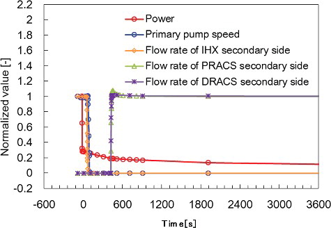
Figure 8. Simulation results of one-dimensional method for loss of off-site power.

The boundary conditions of one pump stick in the primary loop are shown in Figure 9. The primary pump speed of the failed loop-A and the reactor core power decreased simultaneously. After 100 seconds the primary pump speed of the normal side loop B is reduced. Validation analysis has been carried out using these boundary conditions. The analysis results of this event are shown in Figure 10 compared with the test results. In this case immediately after a primary pump stick in the loop A the flow of the loop A is reversed, but after the normal side loop B is tripped the flow rate of the loop A returns to the same level of the normal side loop B. The flow rate of the failed side loop A does not agree with the test result from 400 to 800 seconds. This discrepancy has been caused by a reversed flow occurred in the parallel pipes to be mentioned later in Section 4.3.1. After that, the flow rate of the failed side loop A is larger than that of the normal side loop B from 1000 to 1500 seconds. As a result, the drop of the outlet temperature of the lower plenum in the IHX is delayed because the flow rate through the primary pump of the failed side loop A increases slowly, and the natural circulation flow rate through the primary pump of the failed side loop A increases. Afterwards, the flow rates through the primary pump of the normal side loop B and failed side loop A become almost equal. The first temperature peak is identified in the inner core temperature and outer core temperature because the decrease in the primary flow rate is faster than the decrease of the reactor core power. The analysis results of the inner core temperature, outer core temperature and primary flow rate in both loops show good agreement with the test results as well as in the loss of off-site power case.

Figure 9. Boundary conditions of one-dimensional method for one pump stick in the primary loop.

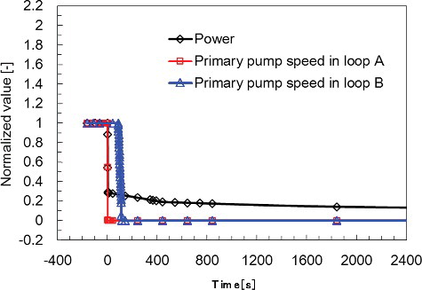
Figure 10. Simulation results of one-dimensional method for one pump stick in the primary loop.

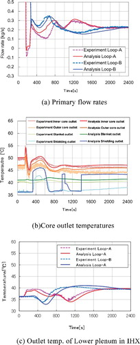
From the above results, the analysis results have shown a fairly good agreement with the test results about decrease of the primary flow rate due to the primary pump coast-down, core flow rate recovery by buoyancy, and inlet and outlet temperatures of the RV in both loops.

4.2.2. PLANDTL sodium test analysis

Figure 11 shows the one-dimensional flow network model to be validated by the PLANDTL sodium tests. This model simulates the primary system and the DHRS of PLANDTL and there are seven channels, each of which represents one fuel subassembly. The one-dimensional safety analysis method has been applied to analysis of the PLANDTL sodium tests, in which the characteristics of the components, such as the pressure losses in the core, heat transfer coefficients in the IHX and PHX, and thermal-hydraulic properties of sodium, have been incorporated into the one-dimensional flow network model as input data.

Figure 11. One-dimensional model for sodium test analysis.

The boundary conditions of the analyses such as the core power decrease, primary pump coast-down curves, inlet flow rates and temperatures of the secondary side of the IHX, air cooler flow rate and air inlet temperature have also been incorporated into the one-dimensional flow network model as input data. The basic scheme of the flow network model applied to the sodium test is the same as that to the SFR.

The validation analyses have been carried out for transient phenomena from a stationary forced circulation state to a natural circulation state of the PRACS, while holding the primary loop to the stationary forced circulation state, called mode transition test, and for transient phenomena from a stationary forced circulation state to a natural circulation state employing an integrated system consisting of the primary sodium system, secondary sodium system of the PRACS and tertiary air cooling system, called all system scram transition test.

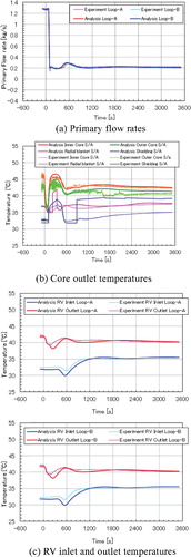
The all system scram transition test is selected in this paper as a typical case. The boundary conditions are shown in Figure 12. The initial core power was set to 500 kW (71 kW/subassembly) which corresponds to 6% of the SFR in terms of the surface heat flux of the fuel pin. The primary flow rate was set at 167 L/min by adjusting the core inlet and outlet temperature difference of about 150 ℃. The primary and secondary flow rates were reduced at 50 seconds from the start of the transient, and then each pump was stopped at 90 seconds from the trip. Heat removal of the secondary system was halted at 2030 seconds from the start of the transient by closing the valve of the secondary sodium circuit. The air cooler damper and vane of the PRACS were opened at 100 seconds from the start of the transient, and then the air cooler blower was started at 240 seconds. Validation analyses have been carried out using these boundary conditions. The analysis results of this test are shown in Figure 13 compared with the test results. The initial value of the PHX sodium inlet and outlet temperature difference between the analyses and tests is almost equal, the initial value of the RV inlet and outlet temperatures and the primary flow rate is nearly the same. However the analysis result of the initial PRACS secondary flow rate is slightly higher. The possible reason of this is that the pressure loss given to the secondary system of the PRACS is not sufficient. The primary flow rate is restored by buoyancy due to an increase of the core outlet temperature and the core outlet temperature rises to about 460 ℃. And then the core outlet temperature, natural circulation flow rate and hot- and cold-leg temperatures in the primary system reach a stationary natural circulation state due to the PRACS.

Figure 12. Boundary conditions of one-dimensional method for all system scram transition test.

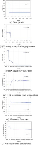
Figure 13. Simulation results of one-dimensional method for all system scram transition test.

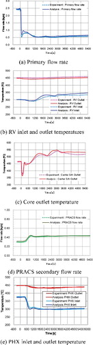
From the above results, it has been confirmed that the validation analyses agree with the sodium test results with nearly the same degree of accuracy as in the analyses of the water tests.

4.3. Validation of three-dimensional fluid flow analysis method

4.3.1. 1/10-scale water test analysis

The three-dimensional fluid flow analysis method has been applied to the 1/10-scale water test, in which the three-dimensional mesh division simulating the geometry of the primary components was constructed for STAR-CD as shown in Figure 14. The total number of meshes is about 5,600,000, and the mesh type employed is basically the hexagonal mesh. The basic scheme of the three-dimensional mesh division applied to the water test analysis is the same as that of the SFR. The boundary condition data are input into the code as in the one-dimensional flow network model. The pressure losses in the pipes and plena and heat transfer coefficients on the inner surfaces of the tubes and structures are calculated based on the standard logarithmic law for smooth walls built in STAR-CD.

Figure 14. Three-dimensional model for water test analyses.

Validation analyses have been made for four typical transient events selected from the DBEs of the SFR, which are (1) loss of off-site power, (2) sodium leakage in the secondary loop, (3) sodium leakage in the secondary side of PRACS, and (4) one pump stick in the primary loop. The analysis results of two typical transient events, (1) and (4), are as follows.

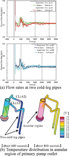
The analysis results of loss of off-site power are shown in Figure 15 compared with the test results. The core outlet temperatures are well simulated in this analysis. The bumpy temperature transient at the radial shielding outlet around 600 seconds is caused by a reverse flow in the radial shield due to unbalance of buoyancy force in the core for a short duration. The small discrepancies of the temperature transients between the analyses and the test results at the core outlet are considered to be caused by temperature mixing due to local convection just above the heating channel outlet. The analysis results of the primary flow rates in the two cold-leg pipes of the primary loop show good agreement with the test results including their oscillating phenomena around 600 seconds after the start of the transient as shown in Figure 16. The reason of the oscillation is speculated as follows: the inlet temperature of the tube bundle in the IHX begins to decrease at 500 seconds when the PHX cooling starts. The temperature in the lower plenum of the IHX once decreases due to the low water temperature of the IHX secondary side and then gradually increases to the IHX inlet (PHX outlet) temperature level. This temperature increase causes the Rayleigh–Taylor instability for an upward flow in the annular region of the IHX as shown in Figure 16. The unstable temperature distribution in the annular region causes an inlet temperature difference between the two parallel pipes of the cold-leg, and it causes unbalance of buoyancy force in the parallel pipes causing a flow oscillation.

Figure 15. Simulation results of three-dimensional method for loss of off-site power.

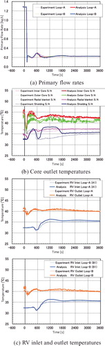
Figure 16. Simulation results of three-dimensional method for loss of off-site power.

The analysis results of one pump stick in the primary loop are shown in Figure 17 compared with the test results. The calculated primary flow rates of both loops and inlet and outlet temperatures of the RV show good agreement with the test results, though the flow rates and the temperatures behave asymmetrically between both loops. Figure 17(a) shows that the timing of the primary flow rate recovery in both loops at about 500 seconds is in good agreement with the test results, while there are some discrepancies with the results of the one-dimensional flow analysis. Figure 17(d) shows that the out-of-phase flow oscillation in the normal side loop B and the reversed flow of the failed side loop A agree well with the test results. The vertical section temperature distributions of the water test apparatus are shown in Figure 18. Due to the effect of the reverse flow generated in the parallel pipes of the failed side loop A at 600 seconds, the upstream temperature of the pipe is high, while the downstream temperature of the pipe is low. When the PHX cooling starts, the reverse flow is eliminated, and gradually a symmetric temperature distribution is restored at 3600 seconds. Although an out-of-phase flow oscillation in the normal side loop B occurs, the coolant flow of the primary system is secured for the above two cases.

Figure 17. Simulation results of three-dimensional method for one pump stick in the primary loop.

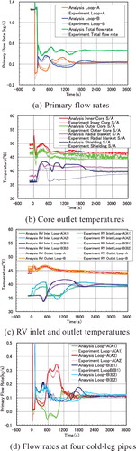
Figure 18. Vertical section temperature distribution of RV upper plenum in one pump stick in the primary loop.

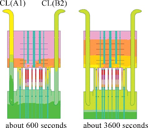
From the above results, the analysis results show good agreement with the test results for the primary flow rates of both loops and the inlet and outlet temperatures of the RV, and with the three-dimensional fluid flow analysis one can evaluate thermal-hydraulics for thermal stratifications and local convections in the primary system.

4.3.2. PLANDTL sodium test analysis

The three-dimensional fluid flow analysis method has been applied to the PLANDTL sodium test. Figure 19 shows the three-dimensional mesh division for STAR-CD to simulate the geometry of the primary system, PRACS and air cooler. The total number of meshes is about 3,900,000. The basic scheme of the sodium test analyses is the same as that of the SFR. The boundary condition data used are the same as those of the one-dimensional safety analysis method. Although the air flow rate of the air cooler has been used as the boundary conditions in the one-dimensional safety analysis method, with the three-dimensional fluid flow analysis method the air inlet flow rate is calculated from the pressure loss and buoyancy in the PRACS.

Figure 19. Three-dimensional fluid modeling for sodium test analysis.

The all system scram transition test is picked up as a typical case in this paper. Like the one-dimensional safety analysis method, Figure 20 shows the primary flow rate, inlet and outlet temperatures of the RV, the secondary flow rate in the PRACS, secondary inlet and outlet temperatures of the PHX and core outlet temperatures compared with the test results. As a result of detailed calculation of the heat loss of the test apparatus, the initial PRACS secondary flow rates show good agreement with the test results. In addition, thanks to precise modeling of the pipe geometry which couples the fuel subassemblies and RV inlet plenum, the core outlet temperatures behavior up to about 1800 seconds from the start of the transient can be simulated better than the one-dimensional safety analysis method. The temperature distributions in the primary system and PRACS at the natural circulation condition (3600 seconds after the trip) are shown in Figure 21. Low temperature coolant stagnates at the bottom of the upper plenum due to the decrease of the core outlet temperature and flow rate, and thermal stratification occurs at the lower level of the UIS. Thermal stratification occurs in the upper plenum of the IHX due to the established PHX cooling. A comparatively strong upward flow occurs in the center of the air cooler tube bundle, and a temperature gradient due to a partial flow is induced in the surrounding air cooler tube bundles. According to the above results, with the three-dimensional fluid flow analysis one can evaluate thermal-hydraulics for thermal stratification in the upper plenum of the RV and IHX which are hard to simulate with the one-dimensional safety analysis method.

Figure 20. Simulation results of three-dimensional method for all system scram transition test.

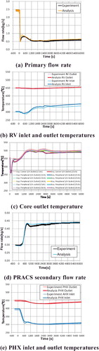
Figure 21. Temperature distributions in PLANDTL under natural circulation condition (at 3600 seconds after the trip).

5. Blind analyses by one- and three-dimensional methods

5.1. Analysis condition

The one-dimensional safety analysis method and the three-dimensional fluid flow analysis method have been validated using the 1/10-scale water tests and the PLANDTL sodium tests described in Chapter 4. In order to demonstrate reliability of these two methods blind analyses using the water test data have been carried out. The following five water test cases have been selected for the blind analyses.

1. Loss of off-site power, and the decay heat has been increased to 1.5 times of the validation analyses.

2. Sodium leakage in the secondary loop, and the decay heat has been increased to 1.5 times of the validation analyses.

3. Sodium leakage in the secondary side of PRACS, and the decay heat has been increased to 1.5 times of the validation analyses.

4. Loss of off-site power, and one PRACS is lost at about 1300 seconds after the DHRS has started (in other words, 1900 seconds after the start of the transient).

5. Loss of off-site power, and the DRACS is lost at about 1300 seconds after the DHRS has started (in other words, 1900 seconds after the start of the transient).

The three water tests from case 1 to case 3 are useful to demonstrate reliability of these methods concerning the similarity ratio to the SFR, i.e. the difference of Re and Pe. The two water tests from case 4 and case 5 are the cases which have not been carried out in Chapter 4 and are useful because they demonstrate adaptability of these methods.

The experimenters have supplied to the analyzers such analysis boundary conditions as the core power decrease, pump coast-down curve, and secondary side inlet flow rate and temperatures of the IHXs, PHXs and DHX. After having received the analysis results the experimenters have compared them and the test results with respect to the flow rates in the primary system and RV inlet and outlet temperatures as representative physical quantities of the natural circulation properties of the primary system, and also evaluated the correlation coefficients between the test results and the analysis results.

5.2. Blind analysis results of the one-dimensional method

The blind analyses of the one-dimensional safety analysis method using the water test data have been carried out for the above-mentioned five cases. Two of them have been picked up in this paper as typical cases and comparisons with the test results are shown in Figure 22.

Figure 22. Blind analysis results of one-dimensional method.

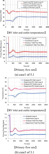
Figure 22(a) shows the analysis results of loss of off-site power with 1.5 times decay heat (case 1 of Section 5.1). The flow rates in the primary system and RV inlet and outlet temperatures show good agreement with the test results to the same degree as the validation analyses described in Section 4.2.1. Figure 22(b) shows the analysis results of loss of off-site power with DRACS loss of function (case 5 of Section 5.1). Heat removal by the DRACS decreases almost to zero after 1900 seconds from the start of the transient, and the flow rates in the primary system increase slightly due to a rise of the RV outlet temperature. These transient phenomena show as good agreement with the test results as in case 1.

5.3. Blind analysis results of the three-dimensional method

The blind analyses of the three-dimensional fluid flow analysis method using the water test data have been carried out for three cases. The blind analysis results of the three-dimensional fluid flow analysis are shown in Figure 23 compared with the test results. Two events selected are the same as those for the one-dimensional analysis.

Figure 23. Blind analysis results of three-dimensional method.

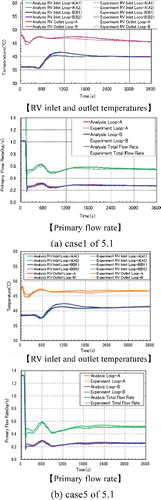
Figure 23(a) shows the analysis results of case 1 of Section 5.1. The flow rates in the primary system and RV inlet and outlet temperatures show good agreement with the test results to the same degree as the validation analyses described in Section 4.3.1. Figure 23(b) shows the analysis results of case 5 of Section 5.1. The flow rates in the primary system and RV inlet and outlet temperatures show as good agreement with the test results as in case 1.

5.4. Correlation of test results and analysis results

Correlation coefficients between the test results and analysis results have been estimated as part of the blind analyses evaluation. The correlation coefficient r can be obtained by the following equation(18) $${\displaystyle r=\frac{{\sum }_{i=1}^n(x_i-\bar{x})(y_i-\bar{y})}{\sqrt{{\sum }_{i=1}^n{(x_i-\bar{x})}^2}\sqrt{{\sum }_{i=1}^n{(y_i-\bar{y})}^2}}}$$(18) :(18) $${\displaystyle r=\frac{{\sum }_{i=1}^n(x_i-\bar{x})(y_i-\bar{y})}{\sqrt{{\sum }_{i=1}^n{(x_i-\bar{x})}^2}\sqrt{{\sum }_{i=1}^n{(y_i-\bar{y})}^2}}}$$(18) where x_i stands for the analysis result and y_i for the test result, and (19) $${\displaystyle \bar{x}=\frac{1}{n}\sum _{i=1}^n{x}_i\bar{y}=\frac{1}{n}\sum _{i=1}^n{y}_i.}$$(19)

The correlation coefficients have been estimated by Equations (18)(18) $${\displaystyle r=\frac{{\sum }_{i=1}^n(x_i-\bar{x})(y_i-\bar{y})}{\sqrt{{\sum }_{i=1}^n{(x_i-\bar{x})}^2}\sqrt{{\sum }_{i=1}^n{(y_i-\bar{y})}^2}}}$$(18) and (19(19) $${\displaystyle \bar{x}=\frac{1}{n}\sum _{i=1}^n{x}_i\bar{y}=\frac{1}{n}\sum _{i=1}^n{y}_i.}$$(19) ) using the data up to 4000 seconds after the primary pump trip for the RV inlet and outlet temperatures and primary flow rate. The sampling time of the measured data is one second. As a result, the correlation coefficients have been obtained as 0.7 or more for all the cases. Consequently, it has been confirmed that there are strong correlations between the test results and analysis results, and reliability of each method has been demonstrated.

6. Conclusion

A new methodology applicable to SFR licensing has been developed consisting of a one-dimensional safety analysis taking into account the temperature flattening effect due to buoyancy force in the core and a three-dimensional fluid flow analysis which can evaluate the thermal-hydraulics for local convections and thermal stratifications in the primary system and DHRS.

These methods have been validated using test results by a water test apparatus and a sodium test loop simulating some typical transient events selected from the DBEs of the SFR. Finally, it has been confirmed that there are strong correlations between the test results and analysis results, and reliability of each method has been demonstrated.

In conclusion, highly reliable methods to analyze natural circulation decay heat removal characteristics have been established.

Nomenclature
ai,j:	=	+1 for inlet and −1 for outlet at the pressure node i (−)
A:	=	heat transfer area per unit length (m2/m)
C:	=	specific heat (J/kg K)
Cμ, Cϵ1 ∼ Cϵ4:	=	constant (−)
Cp:	=	specific heat of the fluid (J/kg K)
E:	=	driving pressure by circulation pumps (Pa)
E:	=	empirical constant for smooth walls (−)
F:	=	pressure loss standardized by the initial flow rate (s/kg m2)
G:	=	mass flow rate (kg/s)
ΔH:	=	buoyancy induced pressure (natural circulation force) (Pa)
Ii:	=	set of flow channels connected to a pressure node i (−)
Jj:	=	set of pressure nodes connected to a flow channel j (−)
k:	=	turbulent kinetic energy (m2/s2)
L:	=	fluid inertia (1/m)
M:	=	mass (kg)
M:	=	mass per unit length (kg/m)
P:	=	pressure (Pa)
P:	=	production of the turbulent kinetic energy due to the strain rate Sij (m2/s)
PB:	=	production of the turbulent kinetic energy due to the buoyancy (m2/s)
Prt:	=	turbulent Prandtl number (−)
qw:	=	heat flux (W/m2)
r:	=	correlation coefficient (−)
S:	=	source of mass (kg/s)
Sij:	=	velocity average strain (−)
Tf:	=	temperature of the fluid adjacent to the wall (K)
Tw:	=	temperature on the wall (K)
uτ:	=	slip velocity on the wall (m/s)
U:	=	heat transfer coefficient (W/m2 K)
U:	=	tangential velocity of the fluid adjacent to the wall (m/s)
V:	=	additional pressure loss due to valves standardized by the initial flow rate (s/kg m2)
x:	=	analysis result (−)
y:	=	test result (−)
Greek letters	=
α:	=	exponent of pressure loss (−)
β:	=	constant (−)
κ:	=	Karman constant (−)
τw:	=	tangential stress (Pa)
ρ:	=	density of the fluid (kg/m3)
δ:	=	distance between the center of the adjacent fluid cell and the wall (m)
ν:	=	kinematic viscosity of the fluid (m2/s)
μt:	=	turbulent eddy viscosity (m2/s)
ϵ:	=	turbulent dissipation rate (m2/s3)
η0:	=	constant (−)
Subscripts	=
i:	=	ith coordinate
j:	=	jth coordinate
p:	=	outer tube coolant
t:	=	tube
s:	=	inner tube coolant
sh:	=	shell
air:	=	atmospheric air
EX:	=	the other fluid heat transfer substances
1:	=	heat transfer between the outer tube coolant and the tube
2:	=	heat transfer between the tube and inner tube coolant
3:	=	heat transfer between the outer tube coolant and the shell
4:	=	heat transfer between the shell and the atmospheric air
5:	=	heat transfer between the atmospheric air and the other heat transfer substances

Acknowledgements

The authors are grateful to Prof. H. Ohashi of the University of Tokyo, Prof. T. Okawa of the University of Electro-Communications and Dr. M. Uotani of Central Research Institute of Electric Power Industry (CRIEPI) for their helpful comments to this study. Special thanks are due to Ms. M. Suemori of Mitsubishi FBR Systems, Inc. (MFBR) for her help in development of the three-dimensional analysis method. The present study includes the results of the R&D project “Development of Natural Circulation Evaluation Methods for Decay Heat Removal” entrusted to MFBR by the Ministry of Education, Culture, Sports, Science and Technology of Japan (MEXT).

Disclosure statement

No potential conflict of interest was reported by the authors.

References

- Kotake S, Sakamoto Y, Mihara T. Development of advanced loop-type fast reactor in Japan. J Nucl Sci Technol. 2010;170:133–147.
- Sawada M, Arikawa H, Mizoo N. Experiment and analysis on natural convection characteristics in the experimental fast reactor Joyo. Nucl Eng Des. 1990;120:341–347.
- Nishimura M, Kamide H, Hayashi K, et al. Transient experiments on fast reactor core thermal-hydraulics and its numerical analysis inter-subassembly heat transfer and inter-wrapper flow under natural circulation conditions. Nucl Eng Des. 2000;200:157–175.
- Yamaguchi A, Oiwa A, Hasegawa T. Plant wide thermal hydraulic analysis of natural circulation test at Joyo with MK-II irradiation core. Proceedings of NURETH-4, Vol. 1; 1989 Oct 10–13; Karlsruhe, Germany.
- Koga T, Murakami T, Eguchi Y, et al. Water test of natural circulation for decay heat removal in JSFR. Proceedings of NURETH-14; 2011 Sep 25–30; Toronto, Canada. No.172.
- Kamide H, Kobayashi J, Ono A, et al. Sodium experiment on fully natural circulation systems for decay heat removal in Japan sodium-cooling fast reactor. Proceedings of NURETH-14; 2011 Sep 25–30; Toronto, Canada. No.179.
- Tenchine D, Pialla D, Fanning TH, et al. International benchmark on the natural convection test in Phenix reactor. Nucl Eng Des. 2013;258:189–198.
- Watanabe O, Oyama K, Endo J, et al. Development of evaluation methodology for natural circulation decay heat removal system in a sodium cooled fast reactor. J Nucl Sci Technol. 2015 (in printing).
- Ohyama K, Watanabe O, Eguchi Y, et al. Decay heat removal system by natural circulation for JSFR. Proceedings of FR09; 2009 Dec 7–10; Kyoto, Japan.
- Yamada F, Ohira H. Numerical simulation of Monju plant dynamics by super-COPD using previous startup tests data. Proceedings of ASME 2010 3rd Joint US-European Fluids Engineering Summer Meeting and 8th International Conference on Nanochannels, Microchannels and Minichannels, FEDSM-ICNMM2010-30287; 2010 Aug 1–5; Montreal, Canada.
- Watanabe O, Kotake S, Kubo S. Study on natural circulation evaluation method for a large FBR. Proceedings of NURETH-8; 1997 Sep 30–Nov 4; Kyoto, Japan. No.12.
- Ninokata H, Efthimiadis A, Todreas NE. Distributed resistance modeling of wire-wrapped rod bundles. Nucl Eng Des. 1987;104:93–102.
- Yamada F, Fukano Y, Nishi H, et al. Development of natural circulation analytical model in super-COPD code and evaluation of core cooling capability in Monju during a station blackout. Am Nucl Soc. 2014;188:292–321.
- STAR-CD, methodology, version 4.14. Computational Dynamics Limited; 2010.
- Yakhot V, Orszag. Renormalization group analysis of turbulence – I: basic theory. J Sci Comput. 1986;1:1–51.
- Yakhot V, Orszag SA, Thangam S, et al. Development of turbulence models for shear flows by a double expansion technique. Phys Fluids. 1992;A4(7):1510–1520.
- Doda N, Oshima H, Kamide H, et al. Development of core hot spot evaluation method for a loop type fast reactor equipped with natural circulation decay heat removal system. J Nucl Sci Technol. ( under review).
- Adams B, Ebeida M, Eldred M, et al. DAKOTA version 5.2 user's manual. Sandia National Laboratories; 2011.