Improvement of molten core–concrete interaction model in debris spreading analysis module with consideration of concrete degradation by heat

ABSTRACT

Understanding the situation inside of the reactors at TEPCO's Fukushima Daiichi Nuclear Power Plant and planning of the methods for debris removal are important for decommissioning the reactors. A debris spreading analysis (DSA) module in the severe accident analysis code SAMPSON has been improved and verified to analyze composite phenomena of molten core (debris) spreading on a reactor containment floor and concrete erosion to the inside of the floor by molten core–concrete interaction (MCCI). The primary models in the DSA module were three-dimensional natural convection with simultaneous spreading, melting and solidification in an open space. In addition to these, the analysis capability has been improved to treat phenomena in a closed space, such as debris eroding laterally under concrete floors at the bottom of the sump pit which is done by an advanced method for boundary processing. A buffer cell for flow analysis, which is defined by a different array variable, is arranged in the same coordinates of the concrete cell (structure cell). Mass, momentum, and the advection term of energy between the debris melt cells and the buffer cells are solved. At the same instant, the heat transfer is calculated between the debris melt cells and the structure cells coexisting side by side with the buffer cells. In this study, technical knowledge regarding changes in physical properties due to thermal degradation of concrete was considered for the prediction of erosion rate, and the DSA module with the models noted above was verified by comparison with erosion data of the core–concrete interaction tests in the OECD/MCCI program. The calculated erosion depth, width, and erosion rate under the concrete floor showed good agreement with the test data and the analysis capability of the module was confirmed.

KEYWORDS:

• Severe accident
• numerical simulation
• safety
• MCCI
• spreading
• moving boundary
• SAMPSON

1. Introduction

In the decommissioning project for TEPCO's Fukushima Daiichi Nuclear Power Plant [1], predictions by computer simulations will be effective for prior evaluation of the failure conditions and for the planning of core melt (debris) removal [2]. One of the issues to predict the relocated debris location and the failure of containment structures is to solve the multidimensional phenomena of spreading of debris with coagulability and debris eroding in a complicated structure, such as the floors equipping sump pit. However, the method of coupled analysis for multidimensional thermal flow of spreading, solidification, melting, and erosion remained to be established.

The debris spreading analysis (DSA) module in the severe accident analysis code SAMPSON [3] has models for three-dimensional (3D) convection with spreading of debris in an open space and boundary transport between the melt and the crust [4]. In addition to these, it has the capability for analyzing quasi-3D floor erosion by debris heat, assuming that the cross-sectional sizes of the erosion area are equal or decrease from the surface downward [5]. However, debris lateral erosion under concrete floors occurs easily at the bottom of the sump pit or due to the existence of a horizontal flow channel under the floors. For instance, in the results from core–concrete interaction (CCI) tests [6] using simulated debris, it was observed that the concrete erosions had complicated configurations. Knowing the debris extent under floors is important for planning debris removal from the containment cavity. Multidimensional and phenomenological modeling approaches for molten core–concrete interaction (MCCI) are needed, even though it is difficult to solve the complex fluid behavior with a free surface, the unmoving wall, and the caving structure while the boundaries move due to spreading, erosion, melting, and solidification.

Previous work briefly described the enhancement of the numerical modeling of thermal flow and showed preliminary validation results. However, a few improvements for the modeling and analysis method have been noted to be needed to enhance the quantitative prediction performance. Specifically, it has been suggested that a change in physical properties of concrete by debris heat during the erosion process should be considered and modeled [7].

The first objective of this study is to improve the DSA module in the SAMPSON code by enhancing the existing MCCI model and incorporating modeling of the thermal degradation effect on the erosion rate, so that it makes a full-3D erosion analysis with high prediction accuracy possible. The second objective is to verify the analysis capability of the improved DSA module through comparison with the CCI test data from the OECD/MCCI Program.

2. Existing models for debris spreading analysis and MCCI

2.1. Analytical methods of the existing DSA module in SAMPSON

Figure 1 shows the analytical regions of each module in the SAMPSON code [5]. The reactor building interior is divided into plural components and modules which have mechanistic models to analyze the objective phenomena. Calculated physical quantities in each module are exchanged and used as the boundary conditions. A steady state is calculated in combination with the ‘In-vessel Thermal Hydraulic Analysis’ (THA) module for in-vessel thermal hydraulic analysis, the ‘Fuel Rods Heat up Analysis’ (FRHA) module and the ‘Containment Vessel Phenomena Analysis’ (CVPA) module for containment thermal hydraulic analysis. When a reactor scram and subsequent core damage occur, the ‘Melt Core Relocation Analysis’ (MCRA) module starts a calculation with the THA module (denoted as the THA2 module) that replaces the core part, and other previously started modules. The ‘Fission Product Release from fuel Analysis’ (FPRA) module and the ‘Fission Product Transportation Analysis’ (FPTA) module which analyzes the FP behavior start working in parallel with the above modules at the stage of core overheating.

Figure 1. Analytical regions of each module in the SAMPSON code [5].

When the core melt and the melt relocation occur, the ‘Debris Coolability Analysis’ module starts and solves the spreading and cooling of debris relocated onto the lower head of the reactor pressure vessel (RPV) in combination with the calculation for thermal load and failure behavior of the RPV lower head wall [8,9]. If RPV failure occurs due to the load and heat of debris, the DSA module starts on receiving the data for the discharged debris onto the pedestal floor of the containment cavity through the CVPA module, and analyzes the debris spreading. The DSA module was originally developed for short-term finer analysis ranging to the time debris spreading stops, and after the spreading stops, the ‘Debris-Concrete Reaction Analysis’ (DCRA) module for long-term analysis of MCCI starts receiving initial condition data from the DSA module. For a balance of the computational speed and the model elaboration, the DSA module has a 3D debris thermal-hydraulic model and a quasi-3D concrete erosion model as the MCCI model for the short term and the DCRA module has models for two-dimensional (2D) erosion for the long term based on the 2D thermal conduction analysis in the existing SAMPSON code.

However, sufficient spatial resolution is needed for prior evaluation of the failure conditions of the containment vessel and for the planning of debris removal, and the erosion model must be advanced to full-3D coordinates of the DSA module for the above-mentioned purpose.

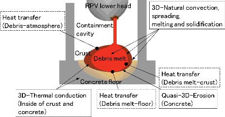
The analytical region, phenomena, and the modeling in the existing DSA module are shown in Figure 2. Composite phenomena of 3D natural convection, spreading, melting, and solidification are analyzed in combination with thermal load by heat transfer and erosion of the concrete floor including the side wall. The analysis method for concrete erosion of the DSA module is that the cross-sectional sizes of the erosion area are equal or decrease from the surface downward. Chemical reactions between debris and eroded concrete are calculated and the chemical heat is added to every melt cell as a heat generation term in the energy equation [10].

Figure 2. Analytical region and modeling in the existing DSA module.

Figure 3 shows the longitudinal section of the analytical mesh and the cell attributions in the existing debris spreading and erosion models in the DSA module. Debris is modeled as single-phase Newtonian fluid arising from convection and it spreads with melting and solidification in an open space. There are two main types of cells from the aspect of cell volume. The first types are convection cells (debris melt cells), crust cells, and structure cells with full cell volume. The second are free surface cells with fragmentary cell volume, and they are arranged on the upper surface of cells of the first types or at the base of the analysis region.

Figure 3. Longitudinal section of debris spreading model and cell attributions.

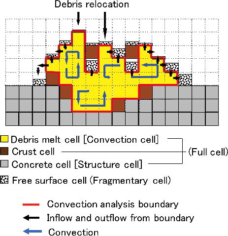
The convection analysis boundary, which is the boundary plane for the 3D region, is lined between the debris melt cells and the solid cells (crust or structure), the debris melt cells and the free surface cells. The free surface cells contacting the convection analysis boundary are used for setting the boundary condition of fixed pressure and free outflow in the flow analysis inside of the convection analysis boundary.

Convection driven by the inertia, the viscosity, the pressure, the liquid head, and the buoyancy in the Navier–Stokes equations for a Newtonian fluid are solved inside of the convection analysis boundary using the simplified marker and cell (SMAC) method [11]. The pressure distribution is calculated by the solver using the incomplete Cholesky conjugate gradient matrix method [12]. For convection analysis boundaries at which the debris melt cells face crust, structure, or free surface cells, matrix rearrangement in the calculation solver of the pressure distribution is processed automatically in the transitional liquid–solid flow.

When solidification occurs at the debris melt cells and they change to crust cells, velocities of the crust cells are forced to be zero and the coefficients of the pressure matrix solver in the next calculation step are rearranged to the wall condition. In a contrasting situation for melting in the crust cells or eroding in the structure cells, the coefficients are rearranged to values of a free flow.

Also, the height function method [13] is applied to solve the external or the internal momentum interaction in the free surface cells outside of the boundary. In this model, the drive force of spreading is calculated in the convection analysis inside of the boundary, and the free surface cells also provide the function of simulating the flow spearhead stop. The free surface cells are set to accept only the horizontal inflow from the convection analysis boundary and only outflow for the vertical direction is allowed.

The mass and momentum conservations in the field equations for the debris melt cells are given as (1) $$\frac{\partial u}{\partial x}+\frac{\partial v}{\partial y}+\frac{\partial w}{\partial z}=0,$$(1) (2) $$\begin{array}{c}{\displaystyle \frac{\partial u}{\partial t}+u\frac{\partial u}{\partial x}+v\frac{\partial u}{\partial y}+w\frac{\partial u}{\partial z}}\hfill \\ {\displaystyle =\frac{1}{\rho }[-\frac{\partial P}{\partial x}+\frac{\partial }{\partial x}\left(\mu \frac{\partial u}{\partial x}\right)+\frac{\partial }{\partial y}\left(\mu \frac{\partial u}{\partial y}\right)}\hfill \\ {\displaystyle +\frac{\partial }{\partial z}\left(\mu \frac{\partial u}{\partial z}\right)]-g\frac{\partial H}{\partial x}-gsin\theta cos\varphi \frac{\partial H}{\partial z},}\hfill \end{array}$$(2) (3) $$\begin{array}{c}{\displaystyle \frac{\partial v}{\partial t}+u\frac{\partial v}{\partial x}+v\frac{\partial v}{\partial y}+w\frac{\partial v}{\partial z}}\hfill \\ {\displaystyle =\frac{1}{\rho }[-\frac{\partial P}{\partial y}+\frac{\partial }{\partial x}\left(\mu \frac{\partial v}{\partial x}\right)+\frac{\partial }{\partial y}\left(\mu \frac{\partial v}{\partial y}\right)}\hfill \\ {\displaystyle +\frac{\partial }{\partial z}\left(\mu \frac{\partial v}{\partial z}\right)]-g\frac{\partial H}{\partial y}-gsin\theta sin\varphi \frac{\partial H}{\partial z},}\hfill \end{array}$$(3) (4) $$\begin{array}{c}{\displaystyle \frac{\partial w}{\partial t}+u\frac{\partial w}{\partial x}+v\frac{\partial w}{\partial y}+w\frac{\partial w}{\partial z}}\hfill \\ {\displaystyle =\frac{1}{\rho }[-\frac{\partial P}{\partial z}+\frac{\partial }{\partial x}\left(\mu \frac{\partial w}{\partial x}\right)+\frac{\partial }{\partial y}\left(\mu \frac{\partial w}{\partial y}\right)}\hfill \\ {\displaystyle +\frac{\partial }{\partial z}\left(\mu \frac{\partial w}{\partial z}\right)]-gcos\theta \frac{\partial H}{\partial z}+K,}\hfill \end{array}$$(4) where u, v, w are the velocities in the x, y, z directions, P is the pressure, μ is the viscosity, H is the sum of liquid head and floor elevation, ϑ is the floor inclination angle, ϕ is the azimuthal direction of maximum floor inclination, and K is the external force of Boussinesq's approximation which simulates the buoyancy.

The field equations of energy conservation for the debris melt cells, crust cells and structure cells are given as (5) $$\begin{array}{c}{\displaystyle \frac{\partial h}{\partial t}+u\frac{\partial h}{\partial x}+v\frac{\partial h}{\partial y}+w\frac{\partial h}{\partial z}}\hfill \\ {\displaystyle =\frac{1}{\rho }\left[\frac{\partial }{\partial x}\left(\lambda \frac{\partial T}{\partial x}\right)+\frac{\partial }{\partial y}\left(\lambda \frac{\partial T}{\partial y}\right)+\frac{\partial }{\partial z}\left(\lambda \frac{\partial T}{\partial z}\right)\right]+Q,}\hfill \end{array}$$(5) where h is the specific enthalpy, λ is the thermal conductivity, and Q is the generation of heat by the radioactive decay and the heat transfer between the debris (debris melt or crust) and the atmospheric fluid, or the debris melt and solid (crust or structure).

The thermal conductions of structure cells are solved by the same energy conservation equation of debris by changing the values of properties, and this makes the thermal conduction calculation between the crust and the concrete possible.

The momentum equation of the liquid head in the height function method in the free surface cells is given as(6) $$\frac{\partial H_f}{\partial t}+u\frac{\partial H_f}{\partial x}+v\frac{\partial H_f}{\partial y}=w,$$(6) where H_f is the liquid head of the free surface cell.

Two assumptions which characterize the spreading and relational motion between the debris melt and the crust are described below.

1. Debris is a continuum body and restricted to the floor surface by gravity. Debris melt cannot scatter into the air and gas entrainment does not occur.

2. Curst can only be transported in the vertical direction.

The first assumption represents that debris melt transporting vacant air cells is collected and integrated into the lowest free surface cells on the floor or on the continuum debris top surface in the vertical direction. The second assumption represents a basic approach to solve the interaction between the debris melt and the crust. It results in the crust waves being proportional to the vertical motion of the debris melt upper surface under the crust.

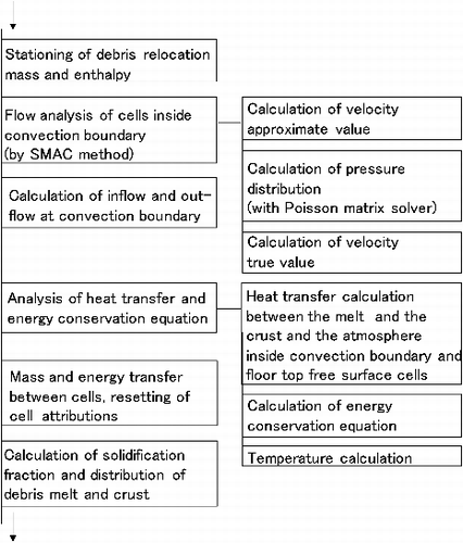
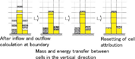
The model concept is the same as described previously [14]. The analytical processes in the debris spreading model are shown in Figure 4. The primary processes consist of positioning debris mass and specific enthalpy, and making the flow, heat transfer and energy conservation analyses, with inflow and outflow at the convection boundary, and finally resetting of cell attribution.

Figure 4. Analytical processes in the debris spreading model.

In the flow analysis, the mass conservation and momentum balance of Equations (1)(1) $$\frac{\partial u}{\partial x}+\frac{\partial v}{\partial y}+\frac{\partial w}{\partial z}=0,$$(1) –(4(4) $$\begin{array}{c}{\displaystyle \frac{\partial w}{\partial t}+u\frac{\partial w}{\partial x}+v\frac{\partial w}{\partial y}+w\frac{\partial w}{\partial z}}\hfill \\ {\displaystyle =\frac{1}{\rho }[-\frac{\partial P}{\partial z}+\frac{\partial }{\partial x}\left(\mu \frac{\partial w}{\partial x}\right)+\frac{\partial }{\partial y}\left(\mu \frac{\partial w}{\partial y}\right)}\hfill \\ {\displaystyle +\frac{\partial }{\partial z}\left(\mu \frac{\partial w}{\partial z}\right)]-gcos\theta \frac{\partial H}{\partial z}+K,}\hfill \end{array}$$(4) ) linked to Equation (6)(6) $$\frac{\partial H_f}{\partial t}+u\frac{\partial H_f}{\partial x}+v\frac{\partial H_f}{\partial y}=w,$$(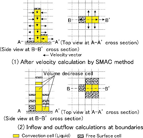6) are solved by the SMAC method. The conceptual view of processes calculating the inflow and outflow is shown in Figure 5. The outflow rate from the inside of the convection boundary to the free surface cells and the inflow rate from the free surface cells to the inside of the convection boundary are calculated and accumulated once. For the debris melt cells next to the convection analysis boundary, inflow from the free surface cells results in the volume decrease based on the modeling of the free surface cells mentioned above.

Figure 5. Calculation of inflow and outflow at convection boundary.

Before the energy conservation equation is solved, the heat transfer between the debris and the crust, the debris and the atmospheric fluid, the debris and the floor concrete, and the concrete and the atmospheric fluid are calculated using methods [15–20] presented in Table 1. They are substituted into the heat generation term Q.

Table 1. Heat transfer forms considered and correlations [15–20].

Attribute of an object	Heat transfer form
Debris–water	Natural convection, nucleate boiling, film boiling, and radiation
Debris–steam	Natural convection and radiation
Debris melt–crust	Natural convection
Debris melt–RPV wall	Natural convection
Debris melt–concrete	Gas film model
Concrete–water	Natural convection, nucleate boiling, film boiling, and radiation
Concrete–steam	Natural convection and radiation

The energy conservation of Equation (5)(5) $$\begin{array}{c}{\displaystyle \frac{\partial h}{\partial t}+u\frac{\partial h}{\partial x}+v\frac{\partial h}{\partial y}+w\frac{\partial h}{\partial z}}\hfill \\ {\displaystyle =\frac{1}{\rho }\left[\frac{\partial }{\partial x}\left(\lambda \frac{\partial T}{\partial x}\right)+\frac{\partial }{\partial y}\left(\lambda \frac{\partial T}{\partial y}\right)+\frac{\partial }{\partial z}\left(\lambda \frac{\partial T}{\partial z}\right)\right]+Q,}\hfill \end{array}$$(5) is solved and the inflow and outflow for energy at the convection boundary are calculated the same as in the flow analysis. The analysis by Equation (5)(5) $$\begin{array}{c}{\displaystyle \frac{\partial h}{\partial t}+u\frac{\partial h}{\partial x}+v\frac{\partial h}{\partial y}+w\frac{\partial h}{\partial z}}\hfill \\ {\displaystyle =\frac{1}{\rho }\left[\frac{\partial }{\partial x}\left(\lambda \frac{\partial T}{\partial x}\right)+\frac{\partial }{\partial y}\left(\lambda \frac{\partial T}{\partial y}\right)+\frac{\partial }{\partial z}\left(\lambda \frac{\partial T}{\partial z}\right)\right]+Q,}\hfill \end{array}$$(5) is for the type of full cell volumes, such as the debris melt cells, crust cells, and the structure cells. The thermal conduction analysis is done among the cells, that is, between the crust cells, the crust cell and the structure cell, and between the structure cells, to make the velocities zero in the left-hand side of Equation (5)(5) $$\begin{array}{c}{\displaystyle \frac{\partial h}{\partial t}+u\frac{\partial h}{\partial x}+v\frac{\partial h}{\partial y}+w\frac{\partial h}{\partial z}}\hfill \\ {\displaystyle =\frac{1}{\rho }\left[\frac{\partial }{\partial x}\left(\lambda \frac{\partial T}{\partial x}\right)+\frac{\partial }{\partial y}\left(\lambda \frac{\partial T}{\partial y}\right)+\frac{\partial }{\partial z}\left(\lambda \frac{\partial T}{\partial z}\right)\right]+Q,}\hfill \end{array}$$(5) . The thermal conductivity between the crust cell and the structure cell is the weighted average in the calculation. The thermal conduction calculation is also done between the debris melt cells.

In the process of mass and energy transfer between the cells, the transported mass and energy between the debris melt cells and the free surface cells calculated by flow analysis and energy conservation analysis are bunched to appropriate cells based on assumption (1). Figure 6 shows the process for the mass and energy transfer between cells and resetting of cell attribution. The outflow mass from debris melt cells to vacant air cells or to free surface cells is transported in the vertical direction. When the free surface cell volume exceeds the full cell volume or the debris melt cell volume drops below the full cell volume, the cell attributions are changed bilaterally. The process shown in Figure 6 is separately done at a later stage of the heat and mass transfer analysis.

Figure 6. Mass and energy transfer between cells and resetting of cell attribution.

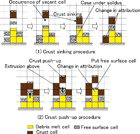
Figure 7 shows the procedure for crust transportation in the resetting of cell attributions. There are two cases in the crust transportation procedure, the crust sinking and the crust push-up. When the debris melt cell volume decreases as shown in Figure 7(1) and a vacant cell is generated directly under the crust cell, the crust sinks to the cell directly below it in incremental steps. On the other hand, when the debris melt cell volume in the cell directly under the crust exceeds the full cell volume, the crust cell is pushed up to the upper portion cell. The free surface cells with differential volume between the exceeded volume and the full cell volume are formed directly under the crust. The cell attribution for which the volume exceeds the full cell volume is changed to the debris melt cell and a free surface cell is put directly above it (Figure 7(2)). Through these procedures and putting the boundary condition of pressure upon the free surface cells under the crust cells in proportion to the crust thickness, debris spreading with melting and solidification can be well simulated, including such behavior as the crust floats on debris melt and waves for hydrodynamic pressure.

Figure 7. Crust transportation and resetting of cell attribution.

Three types of flow stop conditions are applied to characterize the debris spreading. The first is stop of the flow spearhead using the function of the free surface cell that has zero velocity until the cell volume reaches the full cell volume and the cell attribution is changed to a debris melt cell. It can reproduce the effect of the minimum flow thickness. The second is stop of the debris melt cell by considering the flow yield strength [14]. The third is solidification of each full cell volume by the judgment between the fluidity limit solidification fraction and the solidification fraction of cell. It is calculated based on the cell specific enthalpy, the liquidus and solidus using the following equation set. (7) $$\begin{array}{cc}{\displaystyle b=0,}\hfill & \left(h\ge h_l\right)\\ {\displaystyle b=\frac{\left(h-h_s\right)}{\left(h_l-h_s\right)}0,}\hfill & \left(h_l>h>h_s\right)\\ {\displaystyle b=1.0,}\hfill & \left(h\le h_s\right)\end{array}$$(7)

Here b is the solidification fraction, and h_l and h_s are the specific enthalpy at the liquidus and solidus, respectively.

Through the calculation of solidification fraction in Figure 4, the distribution of debris melt and crust are determined by Equation (7)(7) $$\begin{array}{cc}{\displaystyle b=0,}\hfill & \left(h\ge h_l\right)\\ {\displaystyle b=\frac{\left(h-h_s\right)}{\left(h_l-h_s\right)}0,}\hfill & \left(h_l>h>h_s\right)\\ {\displaystyle b=1.0,}\hfill & \left(h\le h_s\right)\end{array}$$(7) . The DSA module can start to solve the entire crust and it is accessible for composite phenomena of the solidification and the remelting.

The solidification fraction b is used not only for the judgment of melting of the crust cells but also the structure cells, and the specific enthalpy at the liquidus and solidus of concrete are applied for the structure cells. When the erosion occurs, the structure cell attribution is changed to the debris melt cell or crust cell in proportion to the surrounding cell attribution, and the appropriate specific enthalpy is given to the cell. The energy difference due to the change in the specific enthalpy of the cell is modified using the internal source term for all debris cells.

On the other hand, solid flow is modeled as analysis options for the solid debris relocation and the solid debris transportation in the DSA module [5]. The first judgment of transport of relocated solid debris is based on the comparison between the surface inclination angle of crust sediment and the angle of rest. The flow calculation sequence is valid as long as the surface inclination angle is more than the angle of rest. The second judgment of solid debris transportation is based on the comparison between the shear stress due to inclination of the debris spearhead and the evaluated value of debris yield strength based on test results or an observation. The flow calculation sequence is functional as crust is allowed to move in the lateral direction locally.

Finally, a new convection boundary for flow analysis of the next calculation step is set distinguishing between the debris melt cell and the crust, structure, and free surface cells.

2.2. Concrete erosion modeling of DSA module and the needs for enhancement

The concrete erosion by debris heat is simulated the same as crust melting when the cell specific enthalpy exceeds the decomposition specific enthalpy. When concrete erosion occurs, the cell attribution is changed to the debris melt cell or crust cell in proportion to the surrounding cell attribution and the appropriate specific enthalpy is given.

Figure 8 shows the difference of the boundary transportation function between the existing erosion model and the advanced erosion model when lateral erosion under a concrete floor occurs. In the existing erosion model shown in the left-hand side of the figure, the erosion was solved in the same meshes of the debris spreading model as shown in Figure 3. Wherein, when debris lateral erosion under concrete floors occurs, the existing erosion model takes a quasi-3D procedure that the eroding sequence is linked to the above structure cells (the blue cells on the left-hand side of Figure 8) to prevent calculation runaway due to the boundary closing.

Figure 8. Boundary transportation function when lateral erosion occurred.

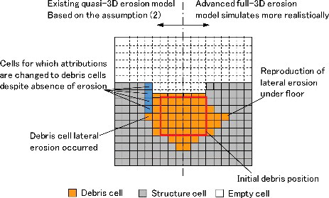
The reason why calculation runaway occurs without the quasi-3D procedure is that the structure cell is processed as a rigid obstacle which cannot be floated and transported vertically on the debris melt and the upper free outflow boundary is not allowed based on assumption (2). It is better for the analysis reproducibility if the number of structure cells linked to the above eroded one is smaller when debris erodes the concrete downward like when the cross-sectional sizes of the erosion area are equal or decrease from the surface downward.

On the other hand, debris lateral erosion occurs easily at the bottom of the sump pit in actual phenomena. For improvement of the analysis reproducibility, the full-3D procedure is able to prevent calculation runaway due to the boundary closing without the eroding sequence linked to the above structure cells as shown on the right-hand side of Figure 8.

In the next section, enhancement of the full-3D concrete erosion model to simulate the lateral erosion finely as shown on the left-hand side of Figure 8 and the verification results are described.

3. Model enhancement and analytical methods

To resolve the above-stated issue, modeling and analysis algorithms are added and amended as follows.

• Addition of the cell attribution of an unmoving structure.

• Prevention of pressure indefiniteness due to the boundary trammel.

• Prevention of movement of the unmoving structure cell.

3.1. Addition of cell attribution of unmoving structure

Table 2 summarizes the differences for the cell attributions and the degree of freedom between the existing model and the advanced model. The debris melt and the free surface cells have a spatial degree of freedom for internal fluid and the cell attribution is changed mutually based on the volume fraction of the liquid or solid. The volume fraction of debris melt cells is 1.0, and that is less than 1.0 for the free surface cells. The crust cells have a degree of freedom for vertical moving only on the debris melt cell across the free surface cell, and they can simulate the crust floating on debris melt. There exists no degrees of freedom for a cell on the floor or a cell connecting to the floor with another crust cell.

Table 2. Cell attributions and the degree of freedom.

Cell attribution	State	Cell freedom and rules in the attribution change
Debris melt	Liquid	• There exists a spatial degree of freedom for internal fluid.• Cell attribution is changed based on the volume fraction of the liquid. (Debris melt → free surface)• Cell attribution is changed based on the specific enthalpy. (Debris melt → crust)
Crust	Solid	• There exists a degree of freedom for a cell moving on a liquid surface of debris melt.• There exists no degree of freedom for a cell on the floor or a cell connecting to the floor with another crust cell.• Cell attribution is changed based on the specific enthalpy. (Crust → debris melt)
Caving structure (Existing model)	Solid	• Cell attribution is changed based on the specific enthalpy. (Structure → debris melt, or crust)• Cell attribution is changed regardless of the specific enthalpy when a cell right under the target cell becomes debris melt, crust, or free surface. (Structure → debris melt, or crust)
Unmoving structure (Advanced model)	Solid	• There exists no degree of freedom for a cell moving on a liquid surface of debris melt.• Cell attribution is changed based on the specific enthalpy. (Structure → debris melt, or crust)• Cell attribution is not changed when a cell right under the cell becomes debris melt, crust, or free surface.
Free surface (including vacant air)	Liquid or solid	• There exists a spatial degree of freedom for internal liquid or solid for liquid inflow.• There exists a spatial degree of freedom for internal gas phase for gas outflow.• Cell attribution is changed based on the volume fraction of the liquid or solid. (Free surface → debris melt)• Phase state of cell (liquid or solid) is judged based on the specific enthalpy.

For a structure cell in the existing model (caving structure), the cell attribution is changed to the debris melt cell or the crust cell regardless of the specific enthalpy when a cell right under the cell becomes a debris melt, crust or free surface cell.

In this study, the function of the existing structure cell (caving structure) is left to the model and the cell attribution of structure in the advanced model (unmoving structure) is newly added. The cell attribution is not changed even when a structure cell right under the cell is eroded and becomes a debris melt cell or a crust cell. To combine the caving structure cells and unmoving structure cells, restrained and unrestrained conditions of the various structures in the containment cavity are well and realistically expressed.

3.2. Prevention of pressure indefiniteness due to boundary trammel

Figure 9 shows a conceptual view of the method to prevent the pressure indefiniteness due to the boundary trammel with respect to the unmoving structure. As an example, in the existing method for the upper crust as a floating object, the free surface cell is set right under the crust cell to be pushed up and the pressure boundary of free outflow is set as the free surface cell; this is shown in Figure 9(1). The boundary pressure of the free surface cell is read as a fixed boundary value from the debris melt cell to set the matrix coefficient as positive and real, and on another front, to set as zero from the free surface cell to the debris melt cell [4].

Figure 9. Conceptual view of the method to prevent pressure indefiniteness.

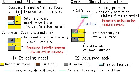
On the other hand, the unmoving structure cell cannot be pushed up and the free surface cell cannot be set right under it because it is a fixed obstacle. Therefore, a buffer cell, which is defined by a different array variable, is arranged in the same coordinate of the unmoving structure cell in the advanced model as shown in Figure 9(2). In the buffer cell, the pressure boundary of free outflow to the debris melt cell is given as the same pressure boundary of the free surface cell. Mass, momentum, and advection of energy between the debris melt cells and the buffer cells are solved with the flow and energy analysis used in the existing model. For heat transfer between the debris melt cells and the structure cells, thermal conductions around the crust cells and the structure cells are solved.

For the buffer cells built outside the analysis region, the mass and energy balance in the overall analysis region becomes exacerbated when the debris mass flowing from the buffer cells increases. To minimize the remaining mass and energy in the buffer cells, a sequence that increases the boundary pressure of the buffer cells in proportion to the cell volume is used for buffer cells. The increase in the boundary pressure qualitatively simulates the reaction force of the debris melt collision into the under-surface of the structure cells.

As a result, pressure of the debris melt region is stabilized and the pressure runaway is prevented through replacement of the fixed boundary by the free outflow boundary to the under-surface of the structure cells.

3.3. Prevention of movement of unmoving structure cell

Figure 10 shows the difference of sequences in an interaction of the structure cell and the crust cell between the existing model and the advanced model. In the situation that the crust cell exists under the unmoving structure cell, something that occurs frequently in the analysis, the structure cell is pushed up in conjunction with the crust when the crust push-up occurs by the sequence shown in Figure 10(1). This is basically true for the sinking behavior also.

Figure 10. Preventing movement of the structure cell above the target crust cell.

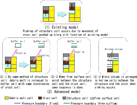
To prevent the movement of primary unmoving structure cells, first, existence of a structure cell above and on the vertical line of the target crust cell is checked when the volume of the free surface cell right under the target crust cell increases and the volume exceeds the full cell volume. If such a structure cell is found, the difference in volume between the debris melt of the free surface cell and the full cell volume is released to the buffer cell located in the same coordinates of the crust cell as shown in Figure 10(2)-1 and 10(2(2) $$\begin{array}{c}{\displaystyle \frac{\partial u}{\partial t}+u\frac{\partial u}{\partial x}+v\frac{\partial u}{\partial y}+w\frac{\partial u}{\partial z}}\hfill \\ {\displaystyle =\frac{1}{\rho }[-\frac{\partial P}{\partial x}+\frac{\partial }{\partial x}\left(\mu \frac{\partial u}{\partial x}\right)+\frac{\partial }{\partial y}\left(\mu \frac{\partial u}{\partial y}\right)}\hfill \\ {\displaystyle +\frac{\partial }{\partial z}\left(\mu \frac{\partial u}{\partial z}\right)]-g\frac{\partial H}{\partial x}-gsin\theta cos\varphi \frac{\partial H}{\partial z},}\hfill \end{array}$$(2) )-2.

Concurrently, a sequence which increases the boundary pressure value in proportion to the debris volume of the buffer cell is provided as a means to minimize the mass and energy in the buffer cell outside the analysis region. The relatively large boundary pressure simulates the debris melt dynamic interaction into the crust lower face and the reaction force. This sequence is also applied when a free surface cell is wedged between the structure cell and the crust cell. On the other hand, when a zero volume cell occurs under the structure cell due to debris melt decrease or crust sinking occurs under the structure cell, the minimum debris volume is apportioned to the cells under the structure cell as shown in Figure 10(2)-3.

4. Verification of advanced model

4.1. Object of analysis

For this study, the capability of the DSA module with the advanced model was verified by published test data using debris which simulated core melt composition; the CCI tests in the OECD/MCCI program were performed to clarify the debris coolability and the concrete erosion in long-term core-concrete interaction in a cavity space [6]. The tests simulated debris for the core melt composition of a pressurized water reactor mixed with concrete, and the decay heat in early stage of the debris relocation onto the containment cavity floor was used. Figure 11 shows the outline configuration, materials and the dimensions of the CCI test section. The horizontal cross section of the cavity was 0.5 m square. The concrete cavity was formed by a basemat and two sidewalls of concrete. The maximum lateral and axial ablation measured are both 0.35 m. Many thermocouples were set in the basemat, sidewalls, and debris space to make it possible to measure the temperature distribution in debris and the spatial distribution of concrete erosion progress. The perpendicular planes of each sidewall were made of MgO refractory walls and tungsten electrodes for direct current heating were installed on the surface with the intermediary material of crushed UO₂ pellets.

Figure 11. Schematic of CCI-2 test section [6].

The cavity test section was designed for 2D core-concrete interaction. However, 3D analysis of this study was thought to be reasonable enough because convection perpendicular to the 2D plane of focus was considered to be non-negligible due to the horizontal aspect ratio of almost 1.0 and the MgO side wall was infusible but not entirely adiabatic.

In the CCI tests, the core–concrete interaction 2 (CCI-2) test was the long period test and concrete erosion depth was very large. Table 3 lists the conditions of the CCI-2 test [6,21]. The concrete type of the CCI-2 test was a limestone/common sand (LCS) and 8.07 wt% LCS was contained in the powder form of the raw material of the debris. The debris melt was generated by the thermite reaction. After an elapsed time 18,048 s during which the concrete erosion had progressed, water was poured directly onto the debris.

Table 3. Conditions of the CCI-2 test [6,21].

Parameters	Test conditions
Initial melt compositions	UO2 : 60.62 wt%ZrO2 : 24.90 wt%Cr : 6.41 wt%Concrete (calcining) : 8.07 wt%
Initial melt mass	400 kg
Initial melt temperature	2153 K
Concrete compositions	Al2O3 : 2.49 wt%CaO : 25.88 wt%Fe2O3 : 1.39 wt%MgO : 11.47 wt%MnO : 0.03 wt%K2O : 0.55 wt%SiO2 : 21.61 wt%Na2O : 0.31 wt%SrO : 0.00 wt%TiO2 : 0.135 wt%SO3 : 0.505 wt%CO2 : 29.71wt%H2O (Free) : 3.255 wt%H2O (Bound) : 1.11 wt%
Power supply	120 kW (0–18,048 s)Decreased with time (18,048--25,386 s)0 kW (25,386 s)
Water pouring start time	18,048 s
Water pouring flow rate	0.002 L/s
Pouring water temperature	293 K

The CCI-2 test results included the time-series data of the melt temperature, the erosion depth, and the heat flux between the debris and water after the water was poured onto the debris. And the general erosion rate, final longitudinal cross-sectional configuration of the concrete erosion, and the local debris material distribution after cool down were represented.

4.2. Analysis conditions

Figure 12 shows the analytical mesh simulating the CCI-2 test section and the MgO top test section shown in Figure 11 was omitted. It should be noted that the erosion progression moves stepwise in increments of the cell size and this occurs in a moment in this model, however in the actual phenomena, concrete erosion progresses continuously from the surface. The erosion of cells does not occur at precisely the same moment for 3D flow and there is a numerical disturbance due to the truncation error, even if the cells are located axisymmetrically. The asynchrony interacts with the 3D flow. In an analogous way, a difference in erosion time between the horizontal and the vertical directions results easily in the case of the cells of a rectangular parallelepiped. To reduce the influence and to improve the simulation accuracy, each cell should be a small cube. The present cell sizes are decided considering the above viewpoint and having a reasonable calculation time. The cells were cubes 0.05 m on each side and the mesh dimension fit the test section.

Figure 12. Analytical mesh and attributions of structure cells.

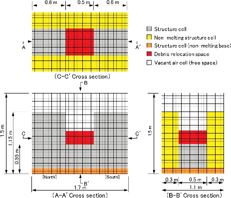
Three types of the structure cells were set, cells for presenting eroded concrete, cells for the non-melting state to give characteristics of the MgO and crushed UO₂ pellets, and cells calculating only thermal conductivity of the analysis base region of the non-melting state. The thermal conduction calculation cells, that is to say the ‘non-melting base’ in the figure, are one of the functions of the DSA module and used for presenting a large heat sink without melting for the base region.

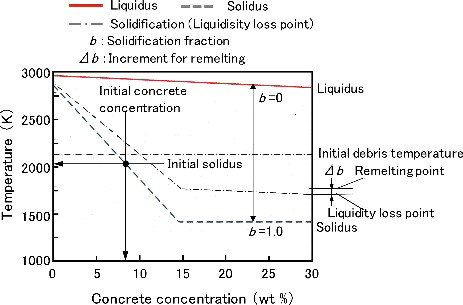
For the property functions, the specific enthalpy of the debris–concrete mixture was calculated as the weighted average [20] of each component enthalpy, UO₂, U₃O₈, Zr, ZrO₂, Fe, FeO, control blades [22], and concrete [23]. The same calculation went for the thermal conductivity, while the viscosity was calculated based on the debris components without dependence on the concrete concentration. Liquidus and solidus of the debris–concrete mixture were obtained from fitting functions depending on the concrete concentration in debris as described briefly in Figure 13 based on other experimental work that showed the depression effect of liquidus and solidus [24], however, they were slightly modified to form a monotonically decreasing function for the calculation stability in this study.

Figure 13. Fitting functions of liquidus and solidus for debris–concrete mixture.

The analytical conditions are shown in Table 4. Both ends of the analytical region width were set to the nearest width of the test section with 0.05 m increments of the cells for an equally spaced analytical mesh. The cell size was determined to put a priority on dimensional accuracy of the cavity. Initial debris was relocated onto the cavity using the function of the spreading model in the DSA module, while the debris state was a solid for the reason of the non-conformity of the enthalpy–temperature function as mentioned later. The specific enthalpy was given as the initial debris temperature corresponding to the CCI-2 test conditions using the property functions at the initial debris composition.

Table 4. Analytical conditions for verification of the CCI-2 test.

Parameters	Conditions
Size of analytical region	1.7 m×1.1 m×1.5 m
Size of cavity space	0.5 m×0.5 m×0.65 m
Analytical mesh of debris spreading and concrete erosion (base region)	34×22×28(34×22×2)
Size of analytical cell of spreading and concrete erosion (base region)	0.05 m×0.05 m×0.05 m(0.05 m×0.05 m×0.05 m)
Debris relocation mass	400 kg
Debris relocation rate	100 kg/s
Initial debris temperature	2153 K
Solidification fraction of liquidity loss (from liquid to solid)	0.8
Solidification fraction at re-melting (from solid to liquid)	0.79
Heat generation rate for debris	0–18,048 s : 120 kW18,048–25,386 s : Decreased fittingpower-time history in test25,386 s≦ : 0 kW
Initial debris composition (wt%)	UO2 : 60.62ZrO2 : 24.90Control material : 6.41Concrete : 8.07
Concrete type	Limestone/common sand (LCS)
Initial concrete temperature	300 K
Water level	0–18,048 s : 0 m18,048 s≦ : 1.0 m
Atmospheric fluid (gas/liquid)	Steam/water
Temperature of steam/water	373 K/373 K
Concrete density	2215 kg/m^3
Concrete thermal conductivity	1.05 W/(m K)

The solidification fraction of liquidity loss is deemed as from 0.5 to 0.7 for instance in non-ferrous alloy [25]. The debris state was solid at the initial debris specific enthalpy contrary to the test data as shown in Figure 13, and a longer time period and an increase in temperature were needed for the remelting by simulated heat generation in the calculation. Although this gave precision to the energy balance, it caused a difference in temperature in the early stage. This condition was attributed to the non-conformity of the enthalpy–temperature function, and two measures were taken to fit the actual phenomena without changing the initial debris temperature. The first was an increase in the solidification fraction of liquidity loss, however the calculation started from the solid (crust) state. The crust was liquidized by heat generation simulating the decay heat. This gave precise in the energy balance, but it caused some difference in temperature in the early stage. The second measure was making a small increment of the solidification fraction for re-melting and that led to minimizing the increase in the temperature difference between the calculation and the test data.

Time-variable heat generation to simulate decay heat in the energy conservation analysis and the ratio of components of the initial debris were set to those of the CCI-2 test [6,21]. The relationship between the specific enthalpy and the temperature of concrete was taken from the literature for LCS concrete [20]. The concrete fraction increased with respect to each erosion judgment of structure cells, and fractions of UO₂, ZrO₂, and control material were once again going down. Pouring water in the test was simulated by changing the water level of the DSA module boundary data. Gas phase of atmospheric fluid was selected as air or steam in the property functions of the DSA module by the model flag. In this verification, steam properties were selected for the gas phase properties of the atmospheric fluid cooling of debris and concrete in consideration of steam generation by the concrete erosion and by water pouring after 18,048 s.

The steam temperature was fixed to 373 K as saturated steam under atmospheric pressure throughout the calculation because the temperature was basically the boundary condition in the DSA module and the change in atmospheric temperatures of nearby debris due to heating by debris was unspecified in this analysis. The pouring water temperature was set to boiling temperature assuming strong heating by debris.

The calculation was continued for 36,000 s of actual time through the water pouring and all debris solidification.

4.3. Consideration for concrete properties

In the preliminary results [7], relatively low debris temperature and the possibility of change in concrete properties by debris heat and the long duration of exposure were pointed out as the cause of underestimations in the concrete erosion rate. In this study, the change of concrete properties by debris heat was considered and the knowledge was reflected in the verification. Nagao and Nakane [26] investigated the change of concrete properties when exposed to high temperature and they tested many kinds of concrete in the range from normal temperature to 873 K. Decreases in the thermal conductivity and density were clarified; in addition, decreases in the compressive strength and elastic coefficient were observed.

For the initial period in the CCI-2 test, it was reported that the relatively low erosion rate in the axial direction and the lateral direction at the early stage were likely to have been caused by a crust protection effect [21]. However, the relatively low erosion rate in the early stage was only seen in the test data at elevation 0 mm of the sidewalls, that is a corner of the cavity, the erosion rates for elevation of +100–+200 mm range (contacting with the middle to top portion of debris) were seen to increase at comparatively higher rates than the data of elevation 0 mm and the latter might not have been due to the crust protection effect. Focusing on the middle to top portion, the following were observed: a relatively low erosion rate in the lateral direction in the early stage until 6000 s and a high rate in the later stage between 6000 and 9000 s. On the other hand, the low rate until 3000 s and the higher rate between 3000 and 6000 s were observed for the axial direction [21]. In this study, the change in erosion rate was considered to be explained by the decrease in the thermal conductivity and density as a potent contributing factor, however this study had no findings to rule out the crust protection effect on the erosion rate at the early stage of the test.

Ideally, these factors should be analyzed as a function of duration and temperature of exposure, and there is a potential possibility that the concrete erosion rate of the CCI-2 test could be reproduced. (8) $$F_i=F_{i0}{f}_i\left(T,t_d\right)$$(8)

Here, F_i is the physical property of an object, such as density or thermal conductivity, F_i0 is the nominal value of the physical property, f_i is the change ratio by the degradation, T is the temperature, t_d is the duration time.

The experimental data [26] and the range are still not enough to apply them to the present analysis, although there is an example to estimate the thermal conductivity of concrete using porosity based on the normal porosity and residual ratio of cement particles and crystalline water obtained from an experiment [27]. Consequently, constant properties were therefore used as a zero-order model in this study as shown in Table 4.

The density of a concrete was decided as the average values between the CCI-2 test data at a normal temperature [6] and the value at high temperature in the literature [26]. The thermal conductivity varies widely depending on the moisture content, water–cement ratio, sand percentage, aggregate density, etc. and the uncertainty is large. There is a report of the thermal conductivity ranging from 1.3 to 1.7 W/(m K) [28], and the typical value of 1.5 W/(m K) at normal temperature was taken in this study. Then, for the present analysis, the thermal conductivity used was the average value at normal temperature and the value at a high temperature calculated by the decreasing ratio of 0.4 estimated roughly from the cited literature [26].

4.4. Verification for analysis capability

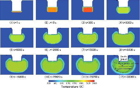
Figure 14 shows the time evolution of the concrete erosion and distribution of debris melt-crust for a longitudinal cross section along the north–south line at the center location between the electrode walls. Debris of crust was relocated in 4 s, and stacked on the cavity floor (Figure 14(1)–14(2)). Remelting of the internal crust occurred and the upper crust floated on debris melt in accord with the method of the debris spreading model (Figure 14(3)). Most of the crust was melted and the first concrete erosion occurred (Figure 14(4)). Part of the cells at a lower corner of the debris were solidified due to the relatively low superheat after erosion cells were changed to debris melt cells, and alternation of the melting and solidification were occasionally observed at the portion. The concrete erosion had progressed in both lateral and axial directions (Figure 14(5)–14(7)), and five layers each 0.05 m thick were eroded until 18,000 s when water was poured on the debris. The upper floating crust was formed by poured water onto the debris upper surface (Figure 14(8)). The upper crust area became large due to the relatively strong cooling by poured water, and the upper crust thickened. Crust thickness of the debris side and bottom was relatively thin by reason of the heat transfer between the debris and the concrete (Figure 14(9)). During the cooling by pouring water, the concrete erosion occurred at the final sixth layer, subsequently, the solidification evolved after the debris melt was surrounded by crust (Figure 14(10)). The lower surface of the upper crust or the upper surface of debris melt showed the concave upward configuration (Figure 14(10) and 14(11)) because upper crust cooling by water was stronger at the center region than the lateral region contacting with concrete which acted as a heat sink. Finally, all debris was solidified and became the crust mass, and the thermal conductivity calculation was continued to the end of the analysis.

Figure 14. Concrete erosion progress and distribution of debris melt-crust.

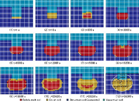
The white solid curve in Figure 14(12) shows the actual edge of concrete erosion and the black solid curve is the debris upper surface at the final stage in the CCI-2 test [6]. The solid line rectangle is the location of the initial cavity wall. The calculated concrete erosion edge agreed rather well with the test data. The analysis capability for the concrete erosion configuration by the DSA module was confirmed, but at the other extreme, two issues became apparent. First, the difference in the final debris surface between the calculation and the test was considered to be the result of mass–volume transformation from eroded concrete to debris. The mixture volume of debris and eroded concrete should be evaluated, in the present analysis, the transformation ratio was one to one. Second, the concrete erosion of the lower surface of the eroded floor over the debris surface for both sides was undervalued. This was derived from the absence of a radiation heat transfer path directly from the debris surface to concrete because the radiation heat of debris passed to the atmospheric fluid in the containment vessel for handling by the CVPA module in the SAMPSON code interface combination.

Figure 15 shows the calculated temperature distribution of the debris and the concrete floor. The internal heating of debris as a crust and cooling from the upper gas environment and thermal conductivity from side and bottom concrete walls were visible at the early stage (Figure 15(1)–15(3)). After the first erosion of the concrete, debris temperature decreased notably (Figure 15(4)). One of the reasons for the low debris temperature was considered to be the mixing with the eroded concrete; however, the temperature of the debris was changed from the temperature of eroded concrete that was given once as the average temperature of debris melt for fitting the continuousness of the actual melting–solidification phenomena to the specific enthalpy decrease in internal heating of all debris to get consistency with the energy balance in the DSA module. This resulted in the decrease in the total debris temperature. Another reason was examined later with the temperature trend data.

Figure 15. Temperature distributions of debris and concrete floor.

With the erosion evolution, temperatures of debris and the concrete near the border were increased, however the temperature of concrete at a site distant from debris was not high. This was due to the relatively low thermal conductivity of concrete (Figure 15(5)–15(8)). After debris melt was surrounded by the crust as shown in Figure 14(10) for instance, the difference between the relatively high temperature of debris melt and the low temperature of the crust periphery was dominant to some degree due to the adiabatic effect from the increase in the crust thickness and the decrease in the heat transfer based on the small temperature difference between the debris melt and the crust surface (Figure 15(9)–15(11)).

No remarkable rise in the temperature at the concrete upper surface was seen even 36,000 s later (Figure 15(12)) in this verification analysis. One of the reasons for this was considered to be the absence of a radiation heat transfer path between the debris upper surface and the eroded lower surface of the floor concrete. The radiation heat transfer path should be considered in the actual reactor analysis to improve the prediction performance, especially to focus attention on the floor strength.

Figure 16 shows the calculated longitudinal velocity vectors of debris melt looking at the typical change in the erosion behavior. Before erosion of the first layer of concrete in the cavity, debris melt flowed downward slowly along the concrete sidewall under the cooling of convective heat transfer and flowed upward along the center region between the two concrete sidewalls. As a result, two asymmetric convection cells were visible in Figure 16(1). After the first layers of both the side and bottom of the cavity were eroded, flow in the convection cells increased to some degree, while there is no change in the cell number and the flow direction (Figure 16(2)). When the second layer was eroded and the debris melt region was expanded, the change in the flow direction was observed in Figure 16(3). It could have numerous possible causes. One cause could be the concrete temperature of the side wall increased at some thicknesses, and the heat transfer between the debris melt and the gas phase over the debris surface became dominant. A second cause could be the change of convection cell formation. A third cause could be the effect of the reaction force simulating the debris melt collision into the under surface of the structure cells. The strikingly large velocity vectors in the upper region of both sides of the debris melt cells were considered to be derived from the reaction force. As the concrete erosion at both the sides and the bottom had progressed from the third layer to the fifth layer, the debris melt region was expanded and the velocity increased with time (Figure 16(4)–16(6)). Large velocities of more than 0.1 m/s (red arrows) were observed at boundaries between the debris melt and the lower surface of the concrete floor.

Figure 16. Calculated velocity vectors of debris melt.

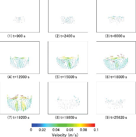
Strong cooling by the pouring water and crust generation caused further increase in the velocity (Figure 16(7)). On the other hand, the velocity decreased overall (Figure 16(8)–16(9)) when generated crust covered the debris melt upper surface. One factor for this was considered as prevention of cooling by the upper crust.

Temperature trends of debris average temperature in the calculation and CCI-2 test [6] are shown in Figure 17. It should be noted that the calculated temperature was the average of debris melt and crust, while the test data were the average of only melt. This might make some difference after water was poured on the debris at 18,048 s.

Figure 17. Comparison between the calculated average debris temperature and the test data [6].

In the early stage of calculation, the debris temperature rose more than in the test data due to the internal heating which simulated melting in the property model in the DSA module. As a result, calculated average debris temperature exceeded the test data until the first concrete layer was eroded. About 1500–2100 s after the calculation started, the first concrete layers of the sides and bottom were eroded, and the average debris temperature had a significant decrease and dropped below the test data until the end. The difference was considered to be due to mismatching of the property functions between the specific enthalpy and the temperature. And the mismatching was caused by the volume change between the calculation and the test data as shown in Figure 14(12). It was clear that the superficial specific enthalpy increased in proportion to the decrease in the volume, although change in volume of the mixture is undefined at the present stage of the analysis.

An eroded structure cell was transformed to a debris cell with the same volume in this model. The debris density was modified in total using reduced debris density depending on the increase in the concrete fraction and initial concrete density. However, volume reduction by debris–concrete mixing was actually as shown in Figure 14(12) and the concrete volume decreased due to the volatile discharge in the decomposition not being considered at the present stage, and that led to a decrease in the specific enthalpy to maintain mass and energy balance. The heat transfer between the debris and the concrete surface decreased and had an influence extending to a reduction of erosion, although the total heat transfer area of the debris slightly increased because the calculated debris volume was larger than the test data. The level of the influence is discussed later, however the goodness of the energy balance made the total eroded mass close to the test data.

Figures 18 and 19 compare the calculated erosion depth and the test data [21] for axial and lateral directions, respectively. While calculated maximum erosion depth for axial and lateral directions at the end agreed with the test data as indicated in Figure 14, the other important aspect of evaluation was the time evolution of erosion. The calculated erosion depth increased at almost a constant rate, however the calculated erosion depth overestimated the test data by 4200 s for the axial direction and by 6600 s for the lateral direction, and the calculations underestimated more than the time especially for the lateral direction. This was due to the use of the constant thermal conductivity and density as concrete properties. Table 5 compares the calculation results and the test data for erosion depth and erosion rate. For the final erosion depth, calculated values were represented stepwise as 0.05 m which depended on the cell size. The calculated erosion depths for axial and lateral directions agreed with the nearest cell boundary of the test data. The erosion rate was calculated as a total value using the time the erosion boundary reached 0.25 m and that included the regions of low erosion rate to high. The ratio of erosion rates between the calculation results and the test data were 0.959 in the axial direction and 0.932 in the lateral direction, respectively. Consequently, they were better than those previously reported [7] and they were judged as reasonable considering the underestimation for less heat transfer between the debris and the concrete due to the comparably low debris temperature as shown in Figure 17.

Figure 18. Comparison between the calculated axial erosion depth and the test data [21].

Figure 19. Comparison between the calculated lateral erosion depth and the test data [21].

Table 5. Comparison of erosion depth and erosion rate between calculation results and test data.

Parameters	Calculation	Test [6]
Axial erosion depth (max.)	0.30 m	0.292 m
Lateral erosion depth (max.)	0.30 m	0.292 m
Axial erosion rate (m/h) (cal.: 0–0.25 m, test: 0–0.241 m)	0.0578	0.0603
Lateral erosion rate (m/h) (cal.: 0–0.25 m, test: 0–0.292 m)	0.0541	0.0580
Ratio between axial erosion rates (cal./test)	0.959
Ratio between lateral erosion rates (cal./test)	0.932

5. Discussion

The full-3D concrete erosion model is a useful method to predict complex and lateral erosion under the concrete floor of the reactor containment vessel. In the verification analysis, the actual edge of concrete erosion was well reproduced and the erosion rate was predicted with considerable accuracy. However, a number of needed model improvements emerged if better prediction performance is to be attained.

5.1. Model addition of radiation heat transfer between debris and concrete lower surface

The concrete erosion of the lower surface of the eroded floor over the debris surface after lateral erosion progressed was undervalued due to the absence of the radiation heat transfer path, as explained using Figure 14(12). Addition of the radiation heat transfer path directly from the debris surface to the concrete lower surface is effective for the improvement of analysis precision for eroded concrete configuration, and also for the proof strength evaluation of concrete floors.

5.2. Optimization of process for pressure boundary setting

The large velocities that extended well beyond 0.1 m/s (red arrows in Figure 16) are considered to occur due to the upward flow toward the buffer cell that was pushed back and turned around horizontally by the boundary pressure simulating the reaction force of the collision with lower surface of the structure cell. The excessive pressure accelerates the surface flow regionally, while it is considered to have an effect on the convection flow and the erosion through the influence on the temperature distribution of debris melt. The boundary pressure was given as large to minimize the residual debris in the buffer cells in proportion to the volume fraction of the cell, and the maximum volume fraction was 13.3% and the average was suppressed to 2.4% at the end of this analysis. Modeling giving the boundary pressure in the buffer cells should be optimized to decrease the influence on the analysis precision by excessive surface flow.

5.3. Improvement of debris–concrete mixing model and reflection to debris properties

Figures 14(12) and 17 suggested the problems of debris volume reduction and underestimation of debris temperature when concrete was mixed with debris. The mixture volume of debris and eroded concrete should be evaluated; for the present analysis, the transformation ratio from concrete volume to debris volume was one to one. First, a method modifying the mixture volume calculated by the concrete concentration and then development of a process for sequential calculation of volume reduction in the current thermo-fluid analysis with rigid cells are needed. Second, local property functions of debris and concrete mixture that depend on the history of melting and solidification should be developed, although the existing property functions were calculated by using an average concentration. Finally, it is desirable to develop a model for the advection and diffusion of concrete in debris melt to simulate the phenomena realistically.

5.4. Application of thermal fatigue properties to concrete properties and erosion criteria

In this study, density and thermal conductivity of concrete were used for the verification analysis as a constant averaging the value at normal temperature and the value at high temperature. Formulation of change of properties by thermal fatigue considering the temperature and the exposure duration are needed to improve the reproducibility of the time change of the erosion rate. In a similar way, the decision criteria of erosion occurrence should better be quantified using a methodology for thermal degradation fatigue damage accumulation.

6. Conclusion

The concrete erosion model for MCCI analysis in the DSA module in the SAMPSON code was improved with consideration of technical knowledge regarding changes in physical properties by thermal degradation of concrete, and the model capability was verified using erosion data for the CCI-2 test in the OECD/MCCI Program.

A buffer cell arranged in the same coordinates of the structure cell was allocated as an unmoving structure in addition to the existing floating crust cell having free surface cell just below it as a caving structure. Mass, momentum, and the advection term of energy between the debris melt cells and the buffer cells were solved. The heat transfer was solved between the debris melt cells and the structure cells, while the thermal conduction was solved around the crust cells and the structure cells. In addition to the model, changes in the thermal conductivity and density were modeled. As a low-order model, the average values between the normal temperature case and the high-temperature case were used in this analysis.

In the verification, calculated erosion depth and configuration of erosion edge well reproduced the test data. Ratios of the erosion rates between the calculation and the test data were 0.959 in the axial direction and 0.932 in the lateral direction, respectively. The capability of the DSA module for high-precision MCCI analysis was confirmed as a primary stage and the issues for advancement were clarified and the DSA module is considered to be useful for evaluating the situation inside of the reactors at TEPCO's Fukushima Daiichi Nuclear Power Plant and planning of the methods for debris removal.

Acknowledgments

This project is being undertaken by Hitachi-GE Nuclear Energy, Ltd. as a member of the International Research Institute for Nuclear Decommissioning which is entrusted with financial sponsorship from the Japanese Ministry of Economy, Trade and Industry.

Disclosure statement

No potential conflict of interest was reported by the authors.

Nomenclature
b:	=	Solidification fraction (-)
g:	=	Gravity constant (m/s2)
H:	=	Liquid head (m)
h:	=	Specific enthalpy (J/kg)
K:	=	External force (m/s2)
P:	=	Pressure (Pa)
Q:	=	Heat generation (W/m3)
T:	=	Temperature (K)
t:	=	Time (s)
u, v, w:	=	Velocity (m/s)
x, y, z:	=	Coordinates (m) or directions
θ:	=	Floor inclination angle (rad)
μ:	=	Viscosity (Pa• s)
λ:	=	Thermal conductivity (W/m•K)
ρ:	=	Density (kg/m3)
ϕ:	=	Azimuthal direction of maximum floor inclination (rad)

References

- Asahi H. Mid-to-long-term roadmap and R& D plan towards the decommissioning of Fukushima Daiichi NPP unit 1-4. In: International Symposium on Decommissioning of TEPCO's Fukushima Daiichi Nuclear Power Plant Unit 1-4; 2012 Mar 14; Tokyo. TEPCO.
- Yamanaka Y. Research plan regarding improvement of simulation code for understanding the status of fuel debris in the reactor. In: International Symposium on Decommissioning of TEPCO's Fukushima Daiichi Nuclear Power Plant Unit 1-4; 2012 Mar 14; Tokyo.
- Ujita H, Satoh, N, Naitoh M, et al. Development of severe accident analysis code SAMPSON in IMPACT project. J Nucl Sci Technol. 1999;36:1076–1088.
- Hidaka M, Sato N, Ujita H. Verification of flow analysis capability in the model of three-dimensional natural convection with simultaneous spreading, melting and solidification for the debris coolability analysis module in the severe accident analysis code ‘SAMPSON’, (II). J Nucl Sci Technol. 2002;39:520–530.
- Hidaka M, Fujii T, Sakai T. Improvements of the debris spreading model in SAMPSON code. In: Proceedings of the ICAPP; 2014 Apr 6–9; Charlotte (NC).
- Farmer MT, Lomperski S, Kilsdonk DJ, et al. OECD MCCI project final report. OECD/MCCI-2005-TR06, 2006 Feb 28.
- Hidaka M, Fujii T, Sakai T. Improvements of the debris spreading model in SAMPSON code. In: Proceedings of the ICAPP; 2015 May 3–6; Nice.
- Ujita H, Hidaka M. Predictive models for gap and ex-vessel cooling in the debris coolability analysis module of SAMPSON for the IMPACT project. In: Proceedings of Second Japan-Korea Symposium on Nuclear Thermal Hydraulic and Safety (NTHAS-2), 2000 Oct 15–18; Fukuoka.
- Yonenaga H, Ujita H, Hidaka M. Development of super simulator ‘IMPACT’ (IX), (2) Debris coolability evaluation in verification for the TMI-2 accident. In: Proceedings of Fall Meeting of the Atomic Energy Society of Japan, 2002 Oct 14–16; Iwaki. Japanese.
- Hidaka M, Sakai T, Fujii T. Assessment of core status of TEPCO's Fukushima Daiichi nuclear power plants (34) Improvement of chemical reaction model in MCCI Analysis. In: Proceedings of Fall Meeting of the Atomic Energy Society of Japan; 2014 Oct 8–10; Kyoto. Japanese.
- Amsden AA, Harlow FH. The SMAC method: a numerical technique for calculating incompressible fluid flow, LA-4370. 1970.
- Meijerink J, Vorst HA. An iterative solution method for linear systems of which the coefficient matrix is a symmetric M-matrix. Math Comp. 1977;31:148–162.
- Shimegi N, Suzuki M, Ishiguro M, et al. Suuchi Ryuutai Rikigaku (numerical fluid dynamics). Tokyo: Asakura Publ.; 1994. p.51–52. Japanese.
- Hidaka M, Goto A, Umino S, et al. VTFS project: development of the lava flow simulation code LavaSIM with a model for three-dimensional convection, spreading and solidification. Geochem Geophys Geosyst. 2005;6:Q07008, doi:10.1029/2004GC000869.
- Holman JP. Heat transfer. (NY): McGraw-Hill Book Company; 1981.
- Theofanous TG, Syri S, Salmassi T, et al. Critical heat flux through curved, downward facing, thick walls. Nucl Eng Des. 1994;151:247–258.
- Cheung FB, Haddad KH, Liu YC. Critical heat flux (CHF) phenomenon on a downward facing curved surface; 1997. (NUREG/CR-6507, PSU/ME-97-7321).
- Nishikawa K, Fujita Y. Dennetsugaku (heat transfer). Tokyo: Rikogakusha Publ.; 1982. p. 183–191. Japanese.
- Jpn. Soc. Mech. Eng. JSME data book: heat transfer. 4th ed. Tokyo: Maruzen; 1986. p. 68–131. Japanese.
- Bradley DR, Gardner DR, Brockmann JE, et al. CORCON-MOD3 an integrated computer model for analysis of molten core-concrete interactions; 1993. (USNRC Report./CR-5843).
- Farmer MT, Lomperski S, Kilsdonk DJ, et al. OECD MCCI project 2-D core concrete interaction (CCI) tests: final report; 2006. (OECD/MCCI-2005-TR05).
- Siefken LJ, Coryell EW, Harvego EA. MATPRO – A library of materials properties for light-water-reactor accident analysis; 2001. (NUREG/CR-6150, Vol. 4, Rev. 2), (INEL-96/0422).
- Sevon T. A heat transfer analysis of the CCI experiment 1-3. Nucl Eng Des. 2008;238:2377–2386.
- Roche MF, Leibowitz L, Fink JK, et al. Solidus and liquidus temperatures of core-concrete mixtures; 1993. (NUREG/CR-6032, ANL-93/9).
- Shibuya A, Arihara K, Nakamura Y. Measurement of apparent viscosity of ferrous and non-ferrous alloys in liquid /solid coexisting state, Fe-C, Sn-Pb, Al-Cu and Fe-Cr-Ni-C alloys. Tetsu-to-Hagane. 1980;66:1550–1556. Japanese.
- Nagao A, Nakane S, Thermal conductivity of the concrete subjected to high temperature. Proc Jpn Concrete Inst. 1990;12(1):395–400. Japanese.
- Lee JY, Kwon YJ, Harada K. A study on the measurements and estimating method of thermal conductivity of various strength concrete at high temperature. In: Summaries of technical papers of Annual Meeting Architectural Institute of Japan. A-2, Fire safety, off-shore engineering and architecture, information systems technology; 2010. Japanese.
- Onmura S, Kominami K, Matsumoto M, et al. Relationship between heat and moisture properties of concrete and strength: Part 1 measurement of equilibrium moisture content. In: Summaries of technical papers of Annual Meeting Architectural Institute of Japan. D-2, Environmental engineering II, Heat, moisture, thermal comfort, natural energy, air flow, ventilation, smoke exhaustion, computational fluid dynamics, indoor air quality heating, cooling and air-conditioning heat and cold sources, piping systems application of building services; 2004. Japanese.