Two-dimensional “transXend” detector with band structure absorbers for third-generation energy-resolved computed tomography with improved spatial resolution

ABSTRACT

Energy-resolved computed tomography (CT) is a method that can generate multiple CT images reconstructed by the X-rays in specific energy ranges. We have previously discussed a lattice absorber type of X-ray detector for energy-resolved CT. We have now developed a band absorber type detector with the aim of improving spatial resolution. We compare spatial resolution and contrast-to-noise ratios for the two types of detectors.

KEYWORDS:

• X-ray
• computed tomography
• unfolding
• spatial resolution
• signal-to-noise ratio

1. Introduction

X-ray computed tomography (CT) is a widely-employed imaging modality. Images are generated from X-ray attenuation coefficients derived from digital radiographic data taken by 360 degree acquisition around a subject. When looking for tumors, as the X-ray attenuation coefficients of normal and cancer tissues show significant overlap, iodinated contrast agent is often injected into blood vessel to accentuate the differences between normal tissues and tumors: tumors have more portion of blood vessel than normal tissues. We estimated that the X-rays passed the iodine thickness of 1–60 μm in 10 mm thick tumor [1].

In conventional CT, X-rays are measured as electric current; the energy information of the X-ray spectrum is not used [2]. In Figure 1, calculated X-ray energy spectra after passing through 100 mm of water and 30 μm of iodine with tube voltages 80 and 120 kVp are shown. Calculations are performed using Birch's formula [3]. As iodine has an absorption K-edge at 33.2 keV, significant dips are observed.

Figure 1. X-ray energy spectra for 80 and 120 kVp tube voltages after passing through 100 mm of water and 30 μm of iodine.

The electric current I induced by the X-ray absorption in the detector used in CT is written as (1) $$I\propto \int E·Y\left(E\right)dE.$$(1)

Here, E is the energy of X-rays, and Y(E) is the number of X-rays with the energy E absorbed by the detector. Comparing two spectra with different tube voltages, the effect of X-ray absorption by iodine is not very obvious by current measurement in the case of higher tube voltage: this is called the “beam hardening effect” [4]. Because of the beam hardening effect, the CT number of iodine becomes smaller when the tube voltage is higher or the subject is thicker. In other words, CT number does not represent the absolute degree of X-ray attenuation by materials in the conventional CT measurement. Because of this situation, CT number is expressed in Hounsfield Units (HU), in which the relative degree of X-ray attenuation by a material is given using CT numbers set at −1000 for air and 0 for water [2].

To avoid the beam hardening effect and to have a CT number inherent to materials under different measurement conditions, the use of the energy information of X-rays is necessary. This kind of measurement, including effective atomic number and electron density estimations, is necessary in tissue segmentation and precise radiation therapy planning.

Methods that employ the energy information in X-ray CT include dual-energy CT, photon counting CT, and energy-resolved CT.

Dual-energy CT performs attenuation measurements twice using two different tube voltages [5]. As an alternative method, a dual layer detector gives linear attenuation coefficients for high and low energy X-rays [6]. The mean energy of X-rays, however, changes according to the thickness of a subject, inserting a degree of ambiguity into the X-ray energy used for the linear attenuation coefficient measurement.

Photon counting CT measures the energy of each X-ray coming into the X-ray detector. The number of X-rays in CT is, however, enormous: up to 10⁹ mm⁻²s⁻¹ in the unattenuated X-ray beam [7]. On the other hand, the number of X-rays should not exceed 0.5×10⁶ s⁻¹ to avoid distortions due to the pulse pileup effect [8]. The number of X-rays coming into a CT detector is too high to allow measurement of the energy of each X-ray. Because of this difficulty, the photon counting CT is under study using CdZnTe detectors with suppressed counting rate [9]. The photon counting CT systems are in the stage of pre-clinical investigation [10]. Further improvement is necessary to compete with dual energy CT [11].

We have developed a new detector system called a “transXend” detector for energy-resolved CT [12]. The transXend detector consists of several segmented detectors aligned in the direction of X-ray incidence. The segmented detectors measure X-rays as electric current. With the previously obtained response functions of the segmented detectors, the X-ray energy distribution is obtained after analysis. Because the X-rays are measured as electric current, the transXend detector does not have the problem of counting rate. With the transXend detector, we have demonstrated distinction between materials [13], effective atomic number measurements [14], CT with two transmission measurements using previously obtained two-dimensional current ratio maps [15], and the possibility of lower dose exposure CT using contrast agents with high atomic numbers such as gold [16].

The applications described above were performed with collimated X-rays and one detector. For the application of the transXend detector for imaging patients, a two-dimensional type of lattice absorber transXend detector was developed with two kinds of strip metal absorbers [17]. The spatial resolution of the CT image, however, was suboptimal: one pixel of the transXend detector was a rectangle with a side length of twice the width of the strip absorber.

We have developed a new configuration of metal absorbers for higher spatial resolution. The spatial resolutions and qualities of CT images taken by the two-dimensional transXend detectors with the previous and the new absorber configurations are compared.

2. Experiment

2.1. Two configurations of two-dimensional transXend detectors

In a previous paper, a transXend detector for cone beam CT used strip absorbers made of Cu and Sn, coupled with a thermo-luminescent plate as a two-dimensional X-ray detector [17]. The Cu and Sn strip absorbers were placed in a lattice pattern as shown in Figure 2(a). The width and thickness of the strip absorbers were 0.5 and 0.1 mm, respectively. As a result, the pixel size of the lattice absorber transXend detector was 1×1 mm².

Figure 2. Schematic drawings of two-dimensional transXend detectors using (a) lattice absorbers, and (b) band absorbers. A pixel of the transXend detector is shown by broken lines for both (a) and (b).

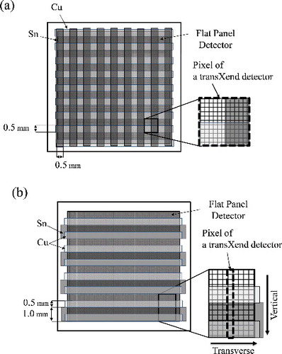
To make the pixel size of the transXend detector smaller, we devised a new absorber configuration to place Cu and Sn strip absorbers parallel as shown in Figure 2(b). We call this detector a “band-transXend detector”. To compare the spatial resolutions of the CT images obtained by the lattice- and band-transXend detectors, the same absorbers were employed: the thicknesses of Cu and Sn were each 0.1 mm. The widths of Cu and Sn absorbers were, however, 0.5 and 1.0 mm, to make four channels with 0.5 mm height: air (channel 1), Cu (channel 2), Sn (channel 3), and Cu and Sn (channel 4). We designate the direction from channel 1 to 4 as vertical, and the direction parallel to the band absorber as transverse. With the band absorbers, the side length of the transXend detector pixel is the same with the one of the pixel of a two-dimensional detector in the traverse direction, i.e., as described below, 48 μm in currently employed flat panel detector (FPD) and the side length in the vertical direction is 2 mm.

2.2. Experimental setup

We employed an X-ray tube (ERESCO 42 MF4®, General Electric Co., Ahrensburg, Germany) and a FPD (Remote RadEye2®, Teledyne Rad-icon Imaging, Sunnyvale CA, USA) as a two-dimensional X-ray detector. The tube voltage and tube current were 120 kVp and 2.3 mA, respectively. The pixel size of a Si photodiode and the sensitive area of the FPD were 48×48 μm² and 49×49 mm², respectively. On the Si photodiode matrix, Gd₂O₂S:Tb (GOS) scintillator plate with the thickness of 140 μm is placed to absorb X-rays. All the measurements were performed with an exposure time of 1.0 s and data were obtained as the mean value of 10 exposures.

The setups for response function and CT measurements are shown in Figure 3. The distances between X-ray tube exit to the phantom and the phantom to the FPD were 85 and 15 cm, respectively.

Figure 3. Schematic drawing of experimental setup. For response function measurements, acrylic slabs and iodine regions shown in the bottom are used instead of a cylindrical acrylic phantom.

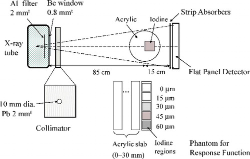
For response function measurements, various concentrations of diluted iodine tincture in acrylic cells were placed in front of acrylic slabs. The thickness ranges of acrylic and iodine were 0–30 mm and 0–60 μm, respectively. For the estimation of the spatial resolutions of lattice- and band-transXend detectors, a 30 mm diameter acrylic phantom with a square hole was fabricated as shown in Figure 4. The 10 mm square hole was filled with diluted iodine with a thickness of 30 μm in a 10 mm X-ray path. The energy ranges for analysis are shown in Table 1.

Figure 4. Details of cylindrical acrylic phantom for spatial resolution measurement. The sizes in the figure are in mm.

Table 1. Assigned energy ranges.

	E1	E2	E3	E4	E5
keV	10.0–33.0	33.0–33.5	33.5–38.5	38.5–70.0	70.0–120.0

2.3. Measurements

Transmission images obtained by the lattice- and band-transXend detectors are shown in Figure 5(a) and 5(b), respectively. In Figure 6, the FPD pixel value profile of the band-transXend detector in the vertical direction is shown. The letters “Air”, “Cu”, “Sn”, and “Cu+Sn” show the FPD pixels in channels 1 to 4.

Figure 5. Transmission measurement images taken by (a) lattice-, (b) band-transXend detectors. In (a) and (b), four and two different channels are enlarged. As the channel values, (a) nine and (b) four pixels at the center are averaged, as shown in the figure.

Figure 6. FPD pixel value profile as a function of pixel number in the vertical direction of the band-transXend detector. “Air”, “Cu”, “Sn”, and “Cu+Sn” in the figure show the FPD pixels under each absorber.

There are 10 FPD pixels (side length: 48 μm) in each channel with the width of 0.5 mm. Among these FPD pixels, the pixels in the border of each channel change their pixel values abruptly. The five to six FPD pixels in the center part of each channel do not have the influence of neighboring channels and have nearly the same values.

As raw data for unfolding X-ray energy distribution, the mean values of nine FPD pixels in the center of each channel were used in the lattice transXend detector to avoid the influence of the neighboring channels, as shown in Figure 5(a) by white lines. Similarly, in the band-transXend detector, the averaged values of four FPD pixels in the vertical direction in the center of each channel were employed as shown in Figure 5(b). Because the FPD pixels described above were chosen by a computer code automatically, nine (3×3) pixels were used in the lattice-transXend detector for avoiding any pixels with inappropriate values.

Transmission profiles taken by the four channels in the lattice- and band-transXend detectors are shown in Figure 7(a) and 7(b), respectively. The symbols in Figure 7(a) are plotted every 1 mm, because the pixel size of the lattice-transXend detector is 1×1 mm². Conversely, the symbols are shown every 20 measurement points in Figure 7(b), because the distance between the measured points is 48 μm in the band-transXend detector.

Figure 7. Transmission measurement data taken by four channels of (a) lattice- and (b) band-transXend detectors. In (b), marks are shown at every 20 measurement points.

2.4. Results of the energy-resolved CT images

Unfolding analysis was performed according to the procedure described by Imamura et al. [18]. The CT images were reconstructed by using the number of X-rays in the energy range E₃ given in Table 1 by the filtered back-projection method [19] as shown in Figure 8. The lines seen in the center from top to bottom in both Figure 8(a) and 8(b) are the images of the adhesive used to join the halves of the cylinder. The three white lines in Figure 8(b) show the locations used for spatial resolution measurements in both images taken using lattice- and band-transXend detectors.

Figure 8. Energy-resolved CT images reconstructed by X-rays in the energy range E₃ of Table 1 measured by (a) lattice- and (b) band-transXend detectors. Three white lines in (b) show the places where spatial resolutions are estimated.

Observing the peripheries of the cylindrical phantom and the square iodine region of the CT images, the one acquired using the band-transXend detector in Figure 8(b) is superior to the one acquired using the lattice-transXend detector in Figure 8(a). Figure 8(b), however, is not smooth, owing to a low signal-to-noise ratio (SNR). This low SNR is caused by the small number of detected X-rays in a pixel of the band-transXend detector. Averaging of FPD pixel values was performed with numbers of combined FPD pixels 3, 5, 7, 11, 13, and 15, in the lateral direction to improve the SNR, and the resulting CT images using the combined transmission data are shown in Figure 9(a)–9(f), respectively.

Figure 9. Energy-resolved CT images reconstructed by X-rays in the energy range E₃ of Table 1 measured by band-transXend detectors. Raw data are obtained by combining (a) 3, (b) 5, (c) 7, (d) 11, (e) 13, and (f) 15 FPD pixels in the transverse direction. CT number is expressed as the linear attenuation coefficient (cm⁻¹).

2.5. Spatial resolution

The spatial resolution of Figure 8(b) is improved over that of Figure 8(a). For the quantitative estimation of the spatial resolution, we employed the edge method [2].

An example of CT number distribution along the line shown in Figure 8(b) is represented by the thick line in Figure 10. The CT number is expressed as the linear attenuation coefficient, not in HU.

Figure 10. Example of spatial resolution estimation. CT number profile along one of the white lines in Figure 8 and the result of fitting are shown by thick and thin lines. The differentiation of fitting result is shown by the dotted line.

The CT number profile is fitted by the following sigmoid function: (2) $$\varsigma \left(x\right)=\frac{a}{1+\mathrm{ exp }\left\{-b\left(x-c\right)\right\}}+d$$(2)

Here, a, b, c, and d are the enlargement ratio, gain, and offsets in the x- and y-direction, respectively. The fit result is shown in Figure 10 by a thin line. Differentiating this line results in a Gaussian-like distribution profile as depicted by the dotted line. We estimated the spatial resolution as the mean of the full widths at half maximum (FWHM) of this dotted line along the three white lines in Figure 8(b). The error of the spatial resolution was estimated as the standard deviation of the three FWHMs.

2.6. Contrast-to-noise ratio

For the quantitative estimation of image quality, contrast-to-noise ratio (CNR) is often used. We use the CNR defined by Guan et al. [20], (3) $$\mathrm{ CNR }=\frac{\left|\mathrm{C}{\mathrm{T}}_{\mathrm{I}}-\mathrm{C}{\mathrm{T}}_{\mathrm{A}}\right|}{\sqrt{{\left(\mathrm{S}{\mathrm{D}}_{\mathrm{I}}\right)}^2+{\left(\mathrm{S}{\mathrm{D}}_{\mathrm{A}}\right)}^2}}.$$(3)

Here, CT_I and CT_A are the averaged CT numbers in the regions of interest (ROI) of iodine and acrylic, respectively, and SD_I, SD_A are their standard deviations. The ROIs are defined by 5×5 mm² squares at the center of the iodine region, and at the corresponding position in the acrylic region on the other side of the adhesive line shown in Figure 8. The estimated spatial resolution and CNR for lattice- and band-transXend detectors as shown in Figure 8 are listed in Table 2.

Table 2. Spatial resolutions (SR), CT numbers (CT), and standard deviations (SD) of iodine (suffix: I) and acrylic (suffix: A) regions and CNR for lattice- and band-transXend detectors.

Detector	SR (mm)	CTI	CTA	SDI	SDA	CNR
Lattice	1.6 ± 0.15	0.68	0.31	0.013	0.010	22 ± 1
Band	0.18 ± 0.04	0.67	0.31	0.32	0.21	0.92 ± 0.00

3. Discussion

3.1. CT images using lattice- and band-transXend detectors

The spatial resolution of the band-transXend detector is 9 × that of the lattice-transXend detector. Conversely, the CNR of the band-transXend detector is far worse than that of the lattice-transXend detector.

The reason for the poor CNR of the band-transXend detector is the large standard deviations in the iodine and acrylic regions, stemming from the small total number of detected X-rays in the pixels: due to the less number of FPD pixels for averaging pixel values in the band-transXend detector than the one in the lattice-transXend detector, the effect of the dark current of FPD to pixel values is more obvious. In Figure 11, FPD pixel value profiles in the center part of the phantom are shown for (a) lattice- and (b) band-transXend detectors. In Figure 11(a), the distance between the measurement points is 1 mm, as described in Section 2.3, and the FPD pixel values of neighboring points have distinct differences. In contrast, the measurement points in Figure 11(b) are distributed more densely. The FPD pixel values fluctuate because the pixel values of the neighboring pixels are similar and the number of incident X-rays into a FPD pixel is small. The pixel values of the band-transXend detector are influenced by the statistics of the numbers of incoming X-rays.

Figure 11. FPD pixel value profiles at the center part of the phantom measured by (a) lattice- and (b) band-transXend detectors.

3.2. CT images using band-transXend detectors with combined FPD pixels

The results of the spatial resolution (circles) and CNR (squares) for the band transXend detector are shown in Figure 12 as a function of combined FPD pixel number. The left y-axis is in ascending order of resolution.

Figure 12. Spatial resolution (circles) and contrast-to-noise ratio (squares) as a function of combined FPD pixel number. Left y-axis is plotted in ascending order of resolution.

The slopes of the borders between the acrylic and iodine regions become gentler by combining FPD pixels. The degrees of slope change depend on the measurement points. As a result, the spatial resolutions and their errors become greater. Combining FPD pixels decreases their number in the ROI. As a result, the standard deviations of FPD pixel values in the ROI, and the error in CNR, increase.

As shown by this figure, 13 combined FPD pixels are necessary for the band-transXend detector to have a CNR value near the CNR of the lattice-transXend detector. In this case, the spatial resolution is 0.8 mm and is still twice as good as that of the lattice-transXend detector.

3.3. CNR and image impression

The CNR value increases as a function of combined FPD pixel number as shown in Figure 12. In contrast, the CT images reconstructed with increasing numbers of combined FPD pixels look increasingly unclear in Figure 9. The CT image with seven combined FPD pixels optimizes sharpness and spatial resolution. CNR is a parameter for easy numerical comparison of image quality but it does not represent image quality as judged by a human observer.

3.4. Pixel size of transXend detector

For improving the spatial resolution of the two-dimensional transXend detector, the lattice-transXend detector with smaller pixel size is a viable method. To make such a lattice-transXend detector, strip absorbers with narrower width should be used. However, four to five FPD pixels change their values abruptly in the border of channels as shown in Figure 6. The FPD pixels from No. 22 to 31 in Figure 6 belong to channel 2. Among these pixels, No. 22 and 23 have the influence of channel 1. Also, FPD pixels from No. 29 to 31 have the influence of channel 3. In other words, the FPD pixels in the distance of nearly 100 to 150 μm from the borders of each side of the channel suffer from the effect of X-ray scatter by the absorbers and cross talk of scintillation photons in the GOS scintillator. With this observation, we can conclude that narrowing the width of the absorber strips has a limitation.

With the consideration above, the band-transXend detector is an effective method to improve the spatial resolution of the two-dimensional transXend detector. Although the number of combined pixels in the transverse direction is 13 to have the same CNR with the one of the lattice-transXend detector, the spatial resolution in this condition is twice better than the lattice-transXend detector.

The pixel size of the band-transXend detector in the vertical direction is 2 mm, i.e., 0.5 mm×4 channels. This value will not be a serious difficulty: in the conventional CT, FPD pixels in the vertical direction are often combined to have greater number of detected X-rays for better statistics to suppress the effect of dark current of FPD pixels [2].

4. Conclusion

The lattice-transXend detector has a pixel size of 1×1 mm² and a spatial resolution of 1.6 mm. We have proposed a band-transXend detector to improve the spatial resolution of energy-resolved CT. The spatial resolution of the band-transXend detector is twice that of the lattice-transXend detector with the same CNR value, indicating its practicality for energy-resolved CT.

Due to the scatter of X-rays and cross talk of scintillation photons, FPD pixels in the border of channels were not used for data acquisition. For decreasing cross talk of photons in the GOS scintillator plate, a scintillator plate made of four kinds of scintillator strips is under development for future study. In this scintillator plate, four different scintillator strips are placed in order repeatedly. The four kinds of scintillator strips replace the Cu and Sn strip absorbers and work as channels 1 to 4. With placing reflectors between neighboring scintillator strips, the photon cross talk will be reduced.

Acknowledgments

The authors would like to thank Prof. K. Hiomi, Tohoku University, for allowing them to use his image reconstruction program. The authors are also grateful to Dr Y. Koba, National Institute of Radiological Sciences, for his fruitful discussions. This work was supported by the Japan Society for the Promotion of Science with a Grant-in-Aid for Scientific Research [grant number 24360394].

Disclosure statement

No potential conflict of interest was reported by the authors.

References

- Kanno I, Uesaka A, Nomiya S, et al. Energy measurement of X-rays in computed tomography for detecting contrast media. J Nucl Sci Technol. 2008;45:15–24 .
- Bushberg JT, Seibert JA, Leidholdt EM Jr., et al. The essential physics of medical imaging. 3rd ed. Philadelphia (PA): Lippincott Williams & Wilkins; 2012.
- Birch R, Marshall M. Computation of bremsstrahlung X-ray spectra and comparison with spectra measured with a Ge(Li) detector. Phys Med Biol. 1979;24:505–517.
- Brooks RA, Di Chiro D. Beam hardening in X-ray reconstructive tomography. Phys Med Biol. 1976;21:390–398.
- Bazalova M, Carrier J-F, Beaulier L, et al. Tissue segmentation in Monte Carlo treatment planning: a simulation study using dual-energy CT images. Radiother Oncol. 2008;86:93–98.
- van Elmpt W, Landry G, Das M, et al. Dual energy CT in radiotherapy: current applications and future outlook. Radiother Oncol. 2016;119:137–144.
- Xu C, Danielsson M, Karlsson S, et al. Preliminary evaluation of a silicon strip detector for photon-counting spectral CT. Nucl Instrum Methods Phys Res. 2012;A 677:45–51.
- Taguchi K, Frey E, Wang X, et al. An analytical model of the effects of pulse pileup on the energy spectrum recorded by energy resolved photon counting x-ray detectors. Med Phys. 2010;37:3957–3970.
- Le HQ, Ducote JL, Molloi S. Radiation dose reduction using a CdZnTe-based computed tomography system: comparison to flat-panel detectors. Med Phys. 2010;37:1225–1236.
- de Vries A, Roessl E, Kneepkens E, et al. Quantitative spectral K-edge imaging in preclinical photon-counting X-ray computed tomography. Invest Radiol. 2015;50:297–304.
- Atak H, Shikhaliev PM. Dual energy CT with photon counting and dual source systems: comparative evaluation. Phys Med Biol. 2015;60:8949–8975.
- Kanno I, Imamura R, Mikami K, et al. A current mode detector for unfolding X-ray energy distribution. J Nucl Sci Technol. 2008;45:1165–1170.
- Kanno I, Imamura R, Yamashita Y, et al. Using energy-resolved X-ray computed tomography with a current mode detector to distinguish materials. Japan J Appl Phys. 2014;53:056601–056604.
- Yamashita Y, Kimura M, Kitahara M, et al. Measurement of effective atomic numbers using energy resolved computed tomography. J Nucl Sci Technol. 2014;51:1256–1263.
- Kanno I, Shima K, Shimazaki H, et al. Computed tomography reconstruction from two transmission measurements for iodine-marked cancer detection. J Nucl Sci Technol. 2013;50;1020–1033.
- Yamashita Y, Shima K, Kanno I, et al. Low-dose exposure energy-resolved X-ray computed tomography using a contrast agent with a high-energy K-edge. J Nucl Sci Technol. 2014;51:91–97.
- Kanno I, Yamashita Y, Kanai E, et al. Two-dimensional “transXend” detector for third-generation energy-resolved computed tomography. J Nucl Sci Technol. 2016;53:258–262.
- Imamura R, Mikami K, Minami Y, et al. Unfolding method with X-ray path length-dependent response functions for computed tomography using X-ray energy information. J Nucl Sci Technol. 2010;47:1075–1082.
- Shepp LA, Logan BF. Fourier reconstruction of a head section. IEEE Trans Nucl Sci. 1974;NS21:21–43.
- Guan H, Gordon R, Zhu Y. Combining various projection access schemes with the algebraic reconstruction technique for low-contrast detection in computed tomography. Phys Med Biol. 1998;43:2413–2421.