Estimation of modeling approximation errors using data assimilation with the minimum variance approach

ABSTRACT

In this paper, we estimate prediction errors owing to approximations in calculation models (modeling approximation error) using the data assimilation method. Correlations between the modeling approximation error and neutronics parameters obtained through calculations are evaluated in test configurations and then the evaluated correlations are used to predict the modeling approximation errors in design configuration. Formulae to estimate the modeling approximation error using the correlations are derived based on the minimum variance approach and the physical interpretation of the formulae is discussed through simple cases. The proposed method is applied in 2 × 2 and 3 × 3 fuel assembly geometries using specifications of the KAIST benchmark problem. The correlation between the modeling approximation error and parameters (neutron leakage in each fuel assembly) is estimated in 2 × 2 fuel assemblies and then the modeling approximation error in 3 × 3 fuel assemblies is predicted using the correlation. The calculation results not only indicate feasibility of the present method, but also suggest a need for further investigation on the assumptions used in the present study, i.e. applicability and robustness of the correlation among different geometries.

KEYWORDS:

• Modeling approximation error
• data assimilation
• minimum variance approach
• uncertainty quantification

1. Introduction

The uncertainty of input parameters and errors in numerical calculation models are considered as major sources of uncertainties in the results of a core analysis. The uncertainty of cross sections and fabrication tolerance are examples of uncertainties in input parameters. In addition, simplified resonance treatment, approximate geometry treatment, spatial homogenization, energy collapsing, and diffusion approximations, which are common in core analyses, are examples of errors in numerical calculation models.

With interest in uncertainty quantification for high-fidelity simulations growing in recent times [1–3], uncertainty estimations of prediction results owing to uncertainties of input parameters and their adjustment are being extensively investigated [1,3,4]. Uncertainties in input data are propagated to calculation results through a simulation model. There are two major approaches to perform uncertainty propagation, i.e. the use of sensitivity and variance-covariance matrices [4], and the use of the random sampling method [5]. In the former approach, a sensitivity matrix, which represents variations of output parameters due to unit variations of input parameters, is estimated and variances of output parameters are calculated by the ‘sandwich formula’ using the sensitivity and variance-covariance matrices. In the latter approach, many perturbed input parameter sets are generated using a variance-covariance matrix and the Monte-Carlo sampling method, and then simulations are carried out using the perturbed input datasets. The simulation results are statistically processed, and then uncertainties and correlations of output data are obtained. The latter approach is especially practical for commercial light water reactor (LWR) analyses owing to the presence of complicated calculation sequences in LWRs and the large number of input and output parameters [5].

There are several types of errors in numerical calculation models – (1(1) $$\begin{array}{c}\hfill {\epsilon }_{\mathrm{est}}=\bar{\epsilon }+\alpha \left(P-\bar{P}\right),\end{array}$$(1) ) simplification of actual physics, (2(2) $$\begin{array}{c}\hfill {\epsilon }_{\mathrm{est}}=\bar{\epsilon }+\mathbf{F}\left(\mathbf{P}-\bar{\mathbf{P}}\right),\end{array}$$(2) ) approximations in fundamental equations that capture actual physics, (3(3) $$\begin{array}{ccc}\hfill \mathbf{E}\left[{\epsilon }_{\mathrm{est}}\right]& =& \mathbf{E}\left[\bar{\epsilon }+\mathbf{F}\left(\mathbf{P}-\bar{\mathbf{P}}\right)\right]\hfill \\ & =& \bar{\epsilon }+\mathbf{FE}\left[\left(\mathbf{P}-\bar{\mathbf{P}}\right)\right]\hfill \\ & =& \bar{\epsilon },\hfill \end{array}$$(3) ) approximations in numerical algorithms (e.g. discretization), and (4(4) $$\begin{array}{ccc}& & \mathbf{V}\left[{\epsilon }_{\mathrm{est}}-\epsilon \right]=\mathbf{E}\left[\left({\epsilon }_{\mathrm{est}}-\epsilon \right){\left({\epsilon }_{\mathrm{est}}-\epsilon \right)}^T\right]\hfill \\ & & =\mathbf{E}\left[\left(\bar{\epsilon }+\mathbf{F}\left(\mathbf{P}-\bar{\mathbf{P}}\right)-\epsilon \right){\left(\bar{\epsilon }+\mathbf{F}\left(\mathbf{P}-\bar{\mathbf{P}}\right)-\epsilon \right)}^T\right]\hfill \\ & & =\mathbf{E}\left[\left(\mathbf{F}\Delta \mathbf{P}-\mathit{\Delta }\epsilon \right){\left(\mathbf{F}\Delta \mathbf{P}-\mathit{\Delta }\epsilon \right)}^T\right]\hfill \\ & & =\mathbf{E}[\mathit{\Delta }\epsilon \Delta {\epsilon }^T-\mathit{\Delta }\epsilon {\left(\mathbf{F}\Delta \mathbf{P}\right)}^T-\mathbf{F}\Delta \mathbf{P}\Delta {\epsilon }^T\hfill \\ & & +\mathbf{F}\Delta \mathbf{P}{\left(\mathbf{F}\Delta \mathbf{P}\right)}^T]\hfill \\ & & =\mathbf{E}[\mathit{\Delta }\epsilon \Delta {\epsilon }^T-\mathit{\Delta }\epsilon \Delta {\mathbf{P}}^T{\mathbf{F}}^T-\mathbf{F}\Delta \mathbf{P}\Delta {\epsilon }^T\hfill \\ & & +\mathbf{F}\Delta \mathbf{P}\Delta {\mathbf{P}}^T{\mathbf{F}}^T]\hfill \\ & & =\mathbf{V}\left[\epsilon \right]-\mathbf{E}\left[\mathit{\Delta }\epsilon \Delta {\mathbf{P}}^T\right]{\mathbf{F}}^T-\mathbf{FE}\left[\Delta \mathbf{P}\Delta {\epsilon }^T\right]\hfill \\ & & +\mathbf{FV}\left[\mathbf{P}\right]{\mathbf{F}}^T,\hfill \end{array}$$(4) ) errors in numerical solutions (e.g. convergence tolerance). The present study mainly focuses on type (3(3) $$\begin{array}{ccc}\hfill \mathbf{E}\left[{\epsilon }_{\mathrm{est}}\right]& =& \mathbf{E}\left[\bar{\epsilon }+\mathbf{F}\left(\mathbf{P}-\bar{\mathbf{P}}\right)\right]\hfill \\ & =& \bar{\epsilon }+\mathbf{FE}\left[\left(\mathbf{P}-\bar{\mathbf{P}}\right)\right]\hfill \\ & =& \bar{\epsilon },\hfill \end{array}$$(3) ), which is considered as the modeling approximation error hereafter. In the present paper, the modeling approximation error is defined as the difference of calculation results using fine and coarse calculation conditions. The systematic error usually referred as the bias is the average of modeling approximation errors, and the standard deviation of modeling approximation errors corresponds to uncertainty.

There are very few researches on the estimation of modeling approximation errors in core analysis. In Ref. [6], the estimation of modeling approximation errors is attempted based on an empirical approach. Differences between detailed (fine) and design (coarse) calculation models, e.g. transport correction, mesh size correction, energy group collapsing correction, are independently estimated. Then, the modeling approximation error is assumed to be proportional to the sum of the corrections. An empirical scaling factor (0.3) is introduced and multiplied to the sum of the corrections to provide an appropriate modeling approximation error. This approach is based on expert observations that (unknown) modeling approximation errors tend to be large when the corrections owing to calculation models are large. This assumption is qualitatively reasonable, but is not fully reliable from a quantitative point of view. In the field of LWR analysis, no systematic study on estimation of modeling approximation errors has been carried out to the best of the authors’ knowledge. In Ref. [3], a framework to estimate modeling approximation errors due to transport calculation methods and multi-group treatment is described. In Ref. [3], modeling approximation errors in lattice cell calculation in a CANDU reactor are quantified through comparison of various calculation methods (e.g. continuous energy Monte-Carlo, multi-group Monte-Carlo, and multi-group SN transport codes) and then evaluated as a covariance matrix of two-group cross sections provided to a core simulator. The covariance matrix of two-group cross sections is used in a core simulator to evaluate uncertainty propagation to core characteristics such as criticality and power peaking factor.

In the present paper, the authors attempt to estimate modeling approximation errors in lattice configurations of typical light water reactors using the data assimilation method [7]. The fundamental idea used in the present study is the utilization of correlations among particular ‘parameters’ and the modeling approximation error. In the field of thermal-hydraulics, various non-dimensional parameters are defined and then used to estimate physical phenomena through interpolation or extrapolation with these parameters [8], which is referred to as scaling. Scaling involves the use of correlation between non-dimensional parameters and physical phenomena. Similarly, correlations between particular parameters (e.g. parameters representing neutronics characteristics of a calculation configuration) and the modeling approximation error obtained in test configurations (e.g. critical assembly) can be used to estimate modeling approximation errors in other configurations (e.g. power reactors). For example, neutron leakage and sensitivity coefficient may be used as particular parameters. Khalik et al. employed a similar concept to determine the calculation bias that is caused by the uncertainty of input parameters [9–12].

The new contributions of the present paper are summarized as follows:

• An equation used to estimate modeling approximation errors is derived using the data assimilation method with the minimum variance approach.

• Difference between a heterogeneous transport calculation and an assembly homogeneous diffusion calculation is considered as the modeling approximation error in the present study and correlation between particular parameters and the modeling approximation error is estimated in LWR lattice geometries. The particular parameters are obtained through assembly homogeneous diffusion calculation.

• The modeling approximation errors in lattice geometries are estimated using the estimation equation and the correlation obtained in other lattice geometries. The estimated modeling approximation errors are compared to actual modeling approximation errors in order to verify the validity of the present method.

The remainder of this paper is organized as follows. In Section 2, the basic idea behind the present study and theoretical derivations of the estimation equation for modeling approximation errors are described. Insights obtained under simplified calculation conditions are also discussed. The general calculation procedure of the present method and discussion on the choice of parameters used for estimation are also presented. In Section 3, calculation conditions, calculation procedures, and calculation results are provided with considerations. Finally, concluding remarks are presented in Section 4.

2. Theory

2.1. Overview

In the present paper, modeling approximation errors are estimated through the data assimilation method, in which correlation among particular parameters and modeling approximation errors is used [7]. There are two major approaches for the application of the data assimilation method, i.e. the maximum likelihood estimation (MLE) and the minimum variance estimation (MVE). In the present paper, the latter approach, i.e. MVE, is used to derive the estimation equation for modeling approximation errors since MVE requires no assumption on probability distributions of uncertainties [13].

The concept of the present approach is shown in Figure 1. $P,\bar{P},{\sigma }_{\mathrm{P}},{\epsilon }_{\mathrm{est}},\bar{\epsilon },\mathrm{and}{\sigma }_{\epsilon }$ are a particular parameter obtained by prediction calculation, average value of the particular parameter, standard deviation of the particular parameter, estimated modeling approximation error, average value of the modeling approximation error, and standard deviation of the modeling approximation error, respectively. The modeling approximation error is defined as the difference between the reference (detail condition) and design (coarse condition) calculations, i.e. reference result – design result. For example, the reference calculation is a multi-group heterogeneous transport calculation based on the method of characteristics (MOC) and the design calculation is a few-group homogeneous diffusion calculation. As discussed in Section 1, correlation between particular parameters and modeling approximation errors may be expected. Any input or output data in design (coarse condition) calculations can be used as the parameter (P), though the selected parameter should have a correlation with the modeling approximation error. As parameters that have a correlation with the modeling approximation error, for example we can consider neutron leakages or sensitivity coefficients. More detailed discussions on the choice of parameters are given in Section 2.5.

Figure 1. Concept of the estimation of the modeling approximation error using correlation.

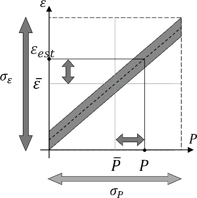
Let us assume that we are aware of a correlation between a particular parameter P and the modeling approximation error ϵ through analysis in various test configurations. Now, we attempt to estimate the modeling approximation error in a design configuration that has similar correlation between the particular parameter and the modeling approximation error. Figure 1 suggest that the modeling approximation error ϵ_est in the design configuration is roughly estimated by Equation (1)(1) $$\begin{array}{c}\hfill {\epsilon }_{\mathrm{est}}=\bar{\epsilon }+\alpha \left(P-\bar{P}\right),\end{array}$$(1) since we know the values of α, $\bar{\epsilon }$, $\bar{P}$ through calculations in various test configurations and P is obtained through a prediction calculation in design configuration. (1) $$\begin{array}{c}\hfill {\epsilon }_{\mathrm{est}}=\bar{\epsilon }+\alpha \left(P-\bar{P}\right),\end{array}$$(1) where α is a constant that represents dependence of modeling approximation error on the particular parameter. It should be noted that more complicated relations between P and ϵ_est can be considered,but it requires additional evaluation of model parameters (α in Equation (1(1) $$\begin{array}{c}\hfill {\epsilon }_{\mathrm{est}}=\bar{\epsilon }+\alpha \left(P-\bar{P}\right),\end{array}$$(1) )).

When the correlation between the particular parameter and the modeling approximation error is not used, the expected uncertainty (standard deviation) of the modeling approximation error, σ^est_ϵ, is identical to σ_ϵ. However, when the correlation is taken into account, the uncertainty of the modeling approximation error reduces depending on the degree of correlation. As shown in Figure 2, the expected uncertainty of the modeling approximation error is smaller when the correlation is strong. However, in the case of weak correlation, reduction of uncertainty of the modeling approximation error is limited, which is an intuitive result.

Figure 2. Highly and weakly correlated cases.

2.2. Derivation of estimation equation using the minimum variance approach

In this subsection, the equation used to estimate the modeling approximation error is derived. Various approaches can be used to establish the estimation equation. Equation (2)(2) $$\begin{array}{c}\hfill {\epsilon }_{\mathrm{est}}=\bar{\epsilon }+\mathbf{F}\left(\mathbf{P}-\bar{\mathbf{P}}\right),\end{array}$$(2) is used in the present study based on the discussion in Section 2.1 and Ref. [13]: (2) $$\begin{array}{c}\hfill {\epsilon }_{\mathrm{est}}=\bar{\epsilon }+\mathbf{F}\left(\mathbf{P}-\bar{\mathbf{P}}\right),\end{array}$$(2) where ${\epsilon }_{\mathrm{est}}$, $\bar{\epsilon }$, F, P, $\mathrm{and}\bar{\mathbf{P}}$ are the estimated modeling approximation errors, the average of modeling approximation errors evaluated in various test configurations, constants determined by the correlation analysis, particular parameters used in and/or obtained by a prediction calculation, and the average of the particular parameters, respectively. ${\epsilon }_{\mathrm{est}}$ and $\bar{\epsilon }$ are column vectors containing n scalar values, P and $\bar{\mathbf{P}}$ are column vectors containing m scalar values, and F is a n × m constant matrix to be determined by the minimum variance method, where m and n are the numbers of particular parameters and neutronics characteristics, respectively, whose modeling approximation error will be estimated.

The average value of ${\epsilon }_{\mathrm{est}}$ is $\bar{\epsilon }$ as shown in Equation (3)(3) $$\begin{array}{ccc}\hfill \mathbf{E}\left[{\epsilon }_{\mathrm{est}}\right]& =& \mathbf{E}\left[\bar{\epsilon }+\mathbf{F}\left(\mathbf{P}-\bar{\mathbf{P}}\right)\right]\hfill \\ & =& \bar{\epsilon }+\mathbf{FE}\left[\left(\mathbf{P}-\bar{\mathbf{P}}\right)\right]\hfill \\ & =& \bar{\epsilon },\hfill \end{array}$$(3) . (3) $$\begin{array}{ccc}\hfill \mathbf{E}\left[{\epsilon }_{\mathrm{est}}\right]& =& \mathbf{E}\left[\bar{\epsilon }+\mathbf{F}\left(\mathbf{P}-\bar{\mathbf{P}}\right)\right]\hfill \\ & =& \bar{\epsilon }+\mathbf{FE}\left[\left(\mathbf{P}-\bar{\mathbf{P}}\right)\right]\hfill \\ & =& \bar{\epsilon },\hfill \end{array}$$(3) where E[x] indicates the average of x. Next, we determine F using the minimum variance method. In Equation (2)(2) $$\begin{array}{c}\hfill {\epsilon }_{\mathrm{est}}=\bar{\epsilon }+\mathbf{F}\left(\mathbf{P}-\bar{\mathbf{P}}\right),\end{array}$$(2) , the estimated modeling approximation error ${\epsilon }_{\mathrm{est}}$ and the actual modeling approximation error $\epsilon$, which is defined by the difference between reference and design calculations, should preferably be as close as possible. The variance in the difference between the estimated modeling approximation error and the actual modeling approximation error is estimated by: (4) $$\begin{array}{ccc}& & \mathbf{V}\left[{\epsilon }_{\mathrm{est}}-\epsilon \right]=\mathbf{E}\left[\left({\epsilon }_{\mathrm{est}}-\epsilon \right){\left({\epsilon }_{\mathrm{est}}-\epsilon \right)}^T\right]\hfill \\ & & =\mathbf{E}\left[\left(\bar{\epsilon }+\mathbf{F}\left(\mathbf{P}-\bar{\mathbf{P}}\right)-\epsilon \right){\left(\bar{\epsilon }+\mathbf{F}\left(\mathbf{P}-\bar{\mathbf{P}}\right)-\epsilon \right)}^T\right]\hfill \\ & & =\mathbf{E}\left[\left(\mathbf{F}\Delta \mathbf{P}-\mathit{\Delta }\epsilon \right){\left(\mathbf{F}\Delta \mathbf{P}-\mathit{\Delta }\epsilon \right)}^T\right]\hfill \\ & & =\mathbf{E}[\mathit{\Delta }\epsilon \Delta {\epsilon }^T-\mathit{\Delta }\epsilon {\left(\mathbf{F}\Delta \mathbf{P}\right)}^T-\mathbf{F}\Delta \mathbf{P}\Delta {\epsilon }^T\hfill \\ & & +\mathbf{F}\Delta \mathbf{P}{\left(\mathbf{F}\Delta \mathbf{P}\right)}^T]\hfill \\ & & =\mathbf{E}[\mathit{\Delta }\epsilon \Delta {\epsilon }^T-\mathit{\Delta }\epsilon \Delta {\mathbf{P}}^T{\mathbf{F}}^T-\mathbf{F}\Delta \mathbf{P}\Delta {\epsilon }^T\hfill \\ & & +\mathbf{F}\Delta \mathbf{P}\Delta {\mathbf{P}}^T{\mathbf{F}}^T]\hfill \\ & & =\mathbf{V}\left[\epsilon \right]-\mathbf{E}\left[\mathit{\Delta }\epsilon \Delta {\mathbf{P}}^T\right]{\mathbf{F}}^T-\mathbf{FE}\left[\Delta \mathbf{P}\Delta {\epsilon }^T\right]\hfill \\ & & +\mathbf{FV}\left[\mathbf{P}\right]{\mathbf{F}}^T,\hfill \end{array}$$(4) where $\mathbf{P}-\bar{\mathbf{P}}=\Delta \mathbf{P}$ and $\epsilon -\bar{\epsilon }=\mathit{\Delta }\epsilon$, and V[x] indicates the variance of x. Note that $\mathbf{V}\left[{\epsilon }_{\mathrm{est}}-\epsilon \right]$ is an n × n matrix.

Based on the minimum variance approach in Ref. [13], a constant matrix F, which minimizes the variance of Equation (4)(4) $$\begin{array}{ccc}& & \mathbf{V}\left[{\epsilon }_{\mathrm{est}}-\epsilon \right]=\mathbf{E}\left[\left({\epsilon }_{\mathrm{est}}-\epsilon \right){\left({\epsilon }_{\mathrm{est}}-\epsilon \right)}^T\right]\hfill \\ & & =\mathbf{E}\left[\left(\bar{\epsilon }+\mathbf{F}\left(\mathbf{P}-\bar{\mathbf{P}}\right)-\epsilon \right){\left(\bar{\epsilon }+\mathbf{F}\left(\mathbf{P}-\bar{\mathbf{P}}\right)-\epsilon \right)}^T\right]\hfill \\ & & =\mathbf{E}\left[\left(\mathbf{F}\Delta \mathbf{P}-\mathit{\Delta }\epsilon \right){\left(\mathbf{F}\Delta \mathbf{P}-\mathit{\Delta }\epsilon \right)}^T\right]\hfill \\ & & =\mathbf{E}[\mathit{\Delta }\epsilon \Delta {\epsilon }^T-\mathit{\Delta }\epsilon {\left(\mathbf{F}\Delta \mathbf{P}\right)}^T-\mathbf{F}\Delta \mathbf{P}\Delta {\epsilon }^T\hfill \\ & & +\mathbf{F}\Delta \mathbf{P}{\left(\mathbf{F}\Delta \mathbf{P}\right)}^T]\hfill \\ & & =\mathbf{E}[\mathit{\Delta }\epsilon \Delta {\epsilon }^T-\mathit{\Delta }\epsilon \Delta {\mathbf{P}}^T{\mathbf{F}}^T-\mathbf{F}\Delta \mathbf{P}\Delta {\epsilon }^T\hfill \\ & & +\mathbf{F}\Delta \mathbf{P}\Delta {\mathbf{P}}^T{\mathbf{F}}^T]\hfill \\ & & =\mathbf{V}\left[\epsilon \right]-\mathbf{E}\left[\mathit{\Delta }\epsilon \Delta {\mathbf{P}}^T\right]{\mathbf{F}}^T-\mathbf{FE}\left[\Delta \mathbf{P}\Delta {\epsilon }^T\right]\hfill \\ & & +\mathbf{FV}\left[\mathbf{P}\right]{\mathbf{F}}^T,\hfill \end{array}$$(4) , is determined. In this approach, the trace, i.e. summation of the diagonal elements in Equation (4)(4) $$\begin{array}{ccc}& & \mathbf{V}\left[{\epsilon }_{\mathrm{est}}-\epsilon \right]=\mathbf{E}\left[\left({\epsilon }_{\mathrm{est}}-\epsilon \right){\left({\epsilon }_{\mathrm{est}}-\epsilon \right)}^T\right]\hfill \\ & & =\mathbf{E}\left[\left(\bar{\epsilon }+\mathbf{F}\left(\mathbf{P}-\bar{\mathbf{P}}\right)-\epsilon \right){\left(\bar{\epsilon }+\mathbf{F}\left(\mathbf{P}-\bar{\mathbf{P}}\right)-\epsilon \right)}^T\right]\hfill \\ & & =\mathbf{E}\left[\left(\mathbf{F}\Delta \mathbf{P}-\mathit{\Delta }\epsilon \right){\left(\mathbf{F}\Delta \mathbf{P}-\mathit{\Delta }\epsilon \right)}^T\right]\hfill \\ & & =\mathbf{E}[\mathit{\Delta }\epsilon \Delta {\epsilon }^T-\mathit{\Delta }\epsilon {\left(\mathbf{F}\Delta \mathbf{P}\right)}^T-\mathbf{F}\Delta \mathbf{P}\Delta {\epsilon }^T\hfill \\ & & +\mathbf{F}\Delta \mathbf{P}{\left(\mathbf{F}\Delta \mathbf{P}\right)}^T]\hfill \\ & & =\mathbf{E}[\mathit{\Delta }\epsilon \Delta {\epsilon }^T-\mathit{\Delta }\epsilon \Delta {\mathbf{P}}^T{\mathbf{F}}^T-\mathbf{F}\Delta \mathbf{P}\Delta {\epsilon }^T\hfill \\ & & +\mathbf{F}\Delta \mathbf{P}\Delta {\mathbf{P}}^T{\mathbf{F}}^T]\hfill \\ & & =\mathbf{V}\left[\epsilon \right]-\mathbf{E}\left[\mathit{\Delta }\epsilon \Delta {\mathbf{P}}^T\right]{\mathbf{F}}^T-\mathbf{FE}\left[\Delta \mathbf{P}\Delta {\epsilon }^T\right]\hfill \\ & & +\mathbf{FV}\left[\mathbf{P}\right]{\mathbf{F}}^T,\hfill \end{array}$$(4) , is minimized by adjusting F as follows: (5) $$\begin{array}{ccc}& & \frac{\partial \mathrm{tr}\left(\mathbf{V}\left[{\epsilon }_{\mathrm{est}}-\epsilon \right]\right)}{\partial \mathbf{F}}=\frac{\partial }{\partial \mathbf{F}}\mathrm{tr}(\mathbf{V}\left[\epsilon \right]-\mathbf{E}\left[\mathit{\Delta }\epsilon \Delta {\mathbf{P}}^T\right]{\mathbf{F}}^T\hfill \\ & & -\mathbf{FE}\left[\Delta \mathbf{P}\Delta {\epsilon }^T\right]+\mathbf{FV}\left[\mathbf{P}\right]{\mathbf{F}}^T)\hfill \\ & & =-\frac{\partial }{\partial \mathbf{F}}\mathrm{tr}\left(\mathbf{E}\left[\mathit{\Delta }\epsilon \Delta {\mathbf{P}}^T\right]{\mathbf{F}}^T\right)-\frac{\partial }{\partial \mathbf{F}}\mathrm{tr}\left(\mathbf{FE}\left[\Delta \mathbf{P}\Delta {\epsilon }^T\right]\right)\hfill \\ & & +\frac{\partial }{\partial \mathbf{F}}\mathrm{tr}\left(\mathbf{FV}\left[\mathbf{P}\right]{\mathbf{F}}^T\right)\hfill \\ & & =-\mathbf{E}\left[\mathit{\Delta }\epsilon \Delta {\mathbf{P}}^T\right]-{\left(\mathbf{E}\left[\Delta \mathbf{P}\Delta {\epsilon }^T\right]\right)}^T\hfill \\ & & +\mathbf{F}\left(\mathbf{V}\left[\mathbf{P}\right]+\mathbf{V}{\left[\mathbf{P}\right]}^T\right)\hfill \\ & & =-2\mathbf{E}\left[\mathit{\Delta }\epsilon \Delta {\mathbf{P}}^T\right]+2\mathbf{FV}\left[\mathbf{P}\right],\hfill \end{array}$$(5) where tr(A) indicates the trace of a matrix A and the following formulae on the trace and transpose of matrices are used: (6) $$\mathbf{tr}\left(\mathbf{A}+\mathbf{B}\right)=\mathbf{tr}\left(\mathbf{A}\right)+\mathbf{tr}\left(\mathbf{B}\right),$$(6) (7) $$\mathbf{tr}\left(\mathbf{AB}\right)=\mathbf{tr}\left(\mathbf{BA}\right),$$(7) (8) $$\frac{\partial \mathbf{tr}\left(\mathbf{AXB}\right)}{\partial \mathbf{X}}={\mathbf{A}}^{\mathit{T}}{\mathbf{B}}^{\mathit{T}},$$(8) (9) $$\frac{\partial \mathbf{tr}\left(\mathbf{A}{\mathbf{X}}^{\mathbf{T}}\mathbf{B}\right)}{\partial \mathbf{X}}=\mathbf{BA},$$(9) (10) $$\frac{\partial \mathbf{tr}\left(\mathbf{XA}{\mathbf{X}}^{\mathit{T}}\right)}{\partial \mathbf{X}}=\mathbf{X}\left(\mathbf{A}+{\mathbf{A}}^{\mathit{T}}\right),$$(10) (11) $${\left(\mathbf{AB}\right)}^{\mathit{T}}={\mathbf{B}}^{\mathit{T}}{\mathbf{A}}^{\mathit{T}}.$$(11)

By forcing $\partial \mathrm{tr}\left(\mathbf{V}\left[{\epsilon }_{\mathrm{est}}-\epsilon \right]\right)/\partial \mathbf{F}=0$, F is obtained as: (12) $$\begin{array}{c}\hfill \mathbf{F}=\mathbf{E}\left[\mathit{\Delta }\epsilon \Delta {\mathbf{P}}^{\mathit{T}}\right]\mathbf{V}{\left[\mathbf{P}\right]}^{-1}.\end{array}$$(12)

Note that a non-singular property of V[P] is assumed. When V[P] is a singular matrix, a generalized inverse is used to derive Equation (12)(12) $$\begin{array}{c}\hfill \mathbf{F}=\mathbf{E}\left[\mathit{\Delta }\epsilon \Delta {\mathbf{P}}^{\mathit{T}}\right]\mathbf{V}{\left[\mathbf{P}\right]}^{-1}.\end{array}$$(12) .

Finally, ${\epsilon }_{\mathrm{est}}$ and its uncertainty, i.e. $\mathbf{V}\left[{\epsilon }_{\mathrm{est}}-\epsilon \right]$, are given by: (13) $$\begin{array}{ccc}\hfill {\epsilon }_{\mathbf{est}}& =& \bar{\epsilon }+\mathbf{F}\left(\mathbf{P}-\bar{\mathbf{P}}\right)\hfill \\ & =& \bar{\epsilon }+\mathbf{E}\left[\mathit{\Delta }\epsilon \Delta {\mathbf{P}}^{\mathit{T}}\right]\mathbf{V}{\left[\mathbf{P}\right]}^{-1}\left(\mathbf{P}-\bar{\mathbf{P}}\right)\hfill \\ & =& \bar{\epsilon }+{\Sigma }_{\mathit{}\epsilon \mathbf{P}}{\left({\Sigma }_{\mathit{PP}}\right)}^{-1}\left(\mathbf{P}-\bar{\mathbf{P}}\right),\hfill \end{array}$$(13) (14) $$\begin{array}{ccc}& & \mathbf{V}\left[{\epsilon }_{\mathbf{est}}-\epsilon \right]=\mathbf{V}\left[\epsilon \right]-\mathbf{E}\left[\mathit{\Delta }\epsilon \Delta {\mathbf{P}}^{\mathit{T}}\right]{\mathbf{F}}^{\mathit{T}}-\mathbf{FE}\left[\Delta \mathbf{P}\Delta {\epsilon }^{\mathit{T}}\right]\hfill \\ & & +\mathbf{FV}\left[\mathbf{P}\right]{\mathbf{F}}^{\mathit{T}}\hfill \\ & & =\mathbf{V}\left[\epsilon \right]-\mathbf{E}\left[\mathit{\Delta }\epsilon \Delta {\mathbf{P}}^{\mathit{T}}\right]{\left(\mathbf{E}\left[\mathit{\Delta }\epsilon \Delta {\mathbf{P}}^{\mathit{T}}\right]\mathbf{V}{\left[\mathbf{P}\right]}^{-1}\right)}^{\mathit{T}}\hfill \\ & & -\mathbf{E}\left[\mathit{\Delta }\epsilon \Delta {\mathbf{P}}^{\mathit{T}}\right]\mathbf{V}{\left[\mathbf{P}\right]}^{-1}\mathbf{E}\left[\Delta \mathbf{P}\Delta {\epsilon }^{\mathit{T}}\right]\hfill \\ & & +\mathbf{E}\left[\mathit{\Delta }\epsilon \Delta {\mathbf{P}}^{\mathit{T}}\right]\mathbf{V}{\left[\mathbf{P}\right]}^{-1}\mathbf{V}\left[\mathbf{P}\right]{\left(\mathbf{E}\left[\mathit{\Delta }\epsilon \Delta {\mathbf{P}}^{\mathit{T}}\right]\mathbf{V}{\left[\mathbf{P}\right]}^{-1}\right)}^{\mathit{T}}\hfill \\ & & =\mathbf{V}\left[\epsilon \right]-\mathbf{E}\left[\mathit{\Delta }\epsilon \Delta {\mathbf{P}}^{\mathit{T}}\right]\mathbf{V}{\left[\mathbf{P}\right]}^{-1}{\left(\mathbf{E}\left[\mathit{\Delta }\epsilon \Delta {\mathbf{P}}^{\mathit{T}}\right]\right)}^{\mathit{T}}\hfill \\ & & -\mathbf{E}\left[\mathit{\Delta }\epsilon \Delta {\mathbf{P}}^{\mathit{T}}\right]\mathbf{V}{\left[\mathbf{P}\right]}^{-1}\mathbf{E}\left[\Delta \mathbf{P}\Delta {\epsilon }^{\mathit{T}}\right]\hfill \\ & & +\mathbf{E}\left[\mathit{\Delta }\epsilon \Delta {\mathbf{P}}^{\mathit{T}}\right]\mathbf{V}{\left[\mathbf{P}\right]}^{-1}\mathbf{V}\left[\mathbf{P}\right]\mathbf{V}{\left[\mathbf{P}\right]}^{-1}{\left(\mathbf{E}\left[\mathit{\Delta }\epsilon \Delta {\mathbf{P}}^{\mathit{T}}\right]\right)}^{\mathit{T}}\hfill \\ & & =\mathbf{V}\left[\epsilon \right]-\mathbf{E}\left[\mathit{\Delta }\epsilon \Delta {\mathbf{P}}^{\mathit{T}}\right]\mathbf{V}{\left[\mathbf{P}\right]}^{-1}\mathbf{E}\left[\Delta \mathbf{P}\Delta {\epsilon }^{\mathit{T}}\right]\hfill \\ & & ={\Sigma }_{\mathit{}\epsilon \epsilon }-{\Sigma }_{\mathit{}\epsilon \mathbf{P}}{\left({\Sigma }_{\mathit{PP}}\right)}^{-1}{\Sigma }_{\mathit{P}\epsilon },\hfill \end{array}$$(14) where $\mathbf{V}\left[\epsilon \right]={\Sigma }_{\mathit{}\epsilon \epsilon },\mathbf{E}\left[\mathit{\Delta }\epsilon \Delta {\mathbf{P}}^{\mathit{T}}\right]={\Sigma }_{\mathit{}\epsilon \mathbf{P}},\mathbf{E}\left[\Delta \mathbf{P}\Delta {\epsilon }^{\mathit{T}}\right]={\Sigma }_{\mathit{P}\epsilon },\mathrm{and}\mathbf{V}\left[\mathbf{P}\right]={\Sigma }_{\mathit{PP}}$

2.3. Discussion under simplified condition

Intuitive interpretations of Equations (13)(13) $$\begin{array}{ccc}\hfill {\epsilon }_{\mathbf{est}}& =& \bar{\epsilon }+\mathbf{F}\left(\mathbf{P}-\bar{\mathbf{P}}\right)\hfill \\ & =& \bar{\epsilon }+\mathbf{E}\left[\mathit{\Delta }\epsilon \Delta {\mathbf{P}}^{\mathit{T}}\right]\mathbf{V}{\left[\mathbf{P}\right]}^{-1}\left(\mathbf{P}-\bar{\mathbf{P}}\right)\hfill \\ & =& \bar{\epsilon }+{\Sigma }_{\mathit{}\epsilon \mathbf{P}}{\left({\Sigma }_{\mathit{PP}}\right)}^{-1}\left(\mathbf{P}-\bar{\mathbf{P}}\right),\hfill \end{array}$$(13) and (14(14) $$\begin{array}{ccc}& & \mathbf{V}\left[{\epsilon }_{\mathbf{est}}-\epsilon \right]=\mathbf{V}\left[\epsilon \right]-\mathbf{E}\left[\mathit{\Delta }\epsilon \Delta {\mathbf{P}}^{\mathit{T}}\right]{\mathbf{F}}^{\mathit{T}}-\mathbf{FE}\left[\Delta \mathbf{P}\Delta {\epsilon }^{\mathit{T}}\right]\hfill \\ & & +\mathbf{FV}\left[\mathbf{P}\right]{\mathbf{F}}^{\mathit{T}}\hfill \\ & & =\mathbf{V}\left[\epsilon \right]-\mathbf{E}\left[\mathit{\Delta }\epsilon \Delta {\mathbf{P}}^{\mathit{T}}\right]{\left(\mathbf{E}\left[\mathit{\Delta }\epsilon \Delta {\mathbf{P}}^{\mathit{T}}\right]\mathbf{V}{\left[\mathbf{P}\right]}^{-1}\right)}^{\mathit{T}}\hfill \\ & & -\mathbf{E}\left[\mathit{\Delta }\epsilon \Delta {\mathbf{P}}^{\mathit{T}}\right]\mathbf{V}{\left[\mathbf{P}\right]}^{-1}\mathbf{E}\left[\Delta \mathbf{P}\Delta {\epsilon }^{\mathit{T}}\right]\hfill \\ & & +\mathbf{E}\left[\mathit{\Delta }\epsilon \Delta {\mathbf{P}}^{\mathit{T}}\right]\mathbf{V}{\left[\mathbf{P}\right]}^{-1}\mathbf{V}\left[\mathbf{P}\right]{\left(\mathbf{E}\left[\mathit{\Delta }\epsilon \Delta {\mathbf{P}}^{\mathit{T}}\right]\mathbf{V}{\left[\mathbf{P}\right]}^{-1}\right)}^{\mathit{T}}\hfill \\ & & =\mathbf{V}\left[\epsilon \right]-\mathbf{E}\left[\mathit{\Delta }\epsilon \Delta {\mathbf{P}}^{\mathit{T}}\right]\mathbf{V}{\left[\mathbf{P}\right]}^{-1}{\left(\mathbf{E}\left[\mathit{\Delta }\epsilon \Delta {\mathbf{P}}^{\mathit{T}}\right]\right)}^{\mathit{T}}\hfill \\ & & -\mathbf{E}\left[\mathit{\Delta }\epsilon \Delta {\mathbf{P}}^{\mathit{T}}\right]\mathbf{V}{\left[\mathbf{P}\right]}^{-1}\mathbf{E}\left[\Delta \mathbf{P}\Delta {\epsilon }^{\mathit{T}}\right]\hfill \\ & & +\mathbf{E}\left[\mathit{\Delta }\epsilon \Delta {\mathbf{P}}^{\mathit{T}}\right]\mathbf{V}{\left[\mathbf{P}\right]}^{-1}\mathbf{V}\left[\mathbf{P}\right]\mathbf{V}{\left[\mathbf{P}\right]}^{-1}{\left(\mathbf{E}\left[\mathit{\Delta }\epsilon \Delta {\mathbf{P}}^{\mathit{T}}\right]\right)}^{\mathit{T}}\hfill \\ & & =\mathbf{V}\left[\epsilon \right]-\mathbf{E}\left[\mathit{\Delta }\epsilon \Delta {\mathbf{P}}^{\mathit{T}}\right]\mathbf{V}{\left[\mathbf{P}\right]}^{-1}\mathbf{E}\left[\Delta \mathbf{P}\Delta {\epsilon }^{\mathit{T}}\right]\hfill \\ & & ={\Sigma }_{\mathit{}\epsilon \epsilon }-{\Sigma }_{\mathit{}\epsilon \mathbf{P}}{\left({\Sigma }_{\mathit{PP}}\right)}^{-1}{\Sigma }_{\mathit{P}\epsilon },\hfill \end{array}$$(14) ) are discussed in this subsection considering a simplified condition. We attempt to estimate the modeling approximation error of a core characteristics (ϵ), e.g. error of k-effective, using two parameters (P1, P2). In this case, the covariance matrices are given by: (15) $$\begin{array}{ccc}\hfill {\Sigma }_{\mathit{}\epsilon \epsilon }& =& {\mathit{\sigma }}_{\mathit{}\epsilon \epsilon },{\Sigma }_{\mathit{}\epsilon \mathbf{P}}=\left(\begin{array}{cc}{\mathit{\sigma }}_{\mathit{}\epsilon \mathbf{P}1}& {\mathit{\sigma }}_{\mathit{}\epsilon \mathbf{P}2}\end{array}\right),{\Sigma }_{\mathit{P}\epsilon }=\left(\begin{array}{c}{\mathit{\sigma }}_{\mathit{P}1\mathit{}\epsilon }\\ {\mathit{\sigma }}_{\mathit{P}2\mathit{}\epsilon }\end{array}\right),\hfill \\ \hfill {\Sigma }_{\mathit{PP}}& =& \left(\begin{array}{cc}{\mathit{\sigma }}_{\mathit{P}1\mathit{P}1}& {\mathit{\sigma }}_{\mathit{P}1\mathit{P}2}\\ {\mathit{\sigma }}_{\mathit{P}2\mathit{P}1}& {\mathit{\sigma }}_{\mathit{P}2\mathit{P}2}\end{array}\right),\hfill \end{array}$$(15) where σ_xy is the covariance between x and y.

In this case, Equations (13)(13) $$\begin{array}{ccc}\hfill {\epsilon }_{\mathbf{est}}& =& \bar{\epsilon }+\mathbf{F}\left(\mathbf{P}-\bar{\mathbf{P}}\right)\hfill \\ & =& \bar{\epsilon }+\mathbf{E}\left[\mathit{\Delta }\epsilon \Delta {\mathbf{P}}^{\mathit{T}}\right]\mathbf{V}{\left[\mathbf{P}\right]}^{-1}\left(\mathbf{P}-\bar{\mathbf{P}}\right)\hfill \\ & =& \bar{\epsilon }+{\Sigma }_{\mathit{}\epsilon \mathbf{P}}{\left({\Sigma }_{\mathit{PP}}\right)}^{-1}\left(\mathbf{P}-\bar{\mathbf{P}}\right),\hfill \end{array}$$(13) and (14(14) $$\begin{array}{ccc}& & \mathbf{V}\left[{\epsilon }_{\mathbf{est}}-\epsilon \right]=\mathbf{V}\left[\epsilon \right]-\mathbf{E}\left[\mathit{\Delta }\epsilon \Delta {\mathbf{P}}^{\mathit{T}}\right]{\mathbf{F}}^{\mathit{T}}-\mathbf{FE}\left[\Delta \mathbf{P}\Delta {\epsilon }^{\mathit{T}}\right]\hfill \\ & & +\mathbf{FV}\left[\mathbf{P}\right]{\mathbf{F}}^{\mathit{T}}\hfill \\ & & =\mathbf{V}\left[\epsilon \right]-\mathbf{E}\left[\mathit{\Delta }\epsilon \Delta {\mathbf{P}}^{\mathit{T}}\right]{\left(\mathbf{E}\left[\mathit{\Delta }\epsilon \Delta {\mathbf{P}}^{\mathit{T}}\right]\mathbf{V}{\left[\mathbf{P}\right]}^{-1}\right)}^{\mathit{T}}\hfill \\ & & -\mathbf{E}\left[\mathit{\Delta }\epsilon \Delta {\mathbf{P}}^{\mathit{T}}\right]\mathbf{V}{\left[\mathbf{P}\right]}^{-1}\mathbf{E}\left[\Delta \mathbf{P}\Delta {\epsilon }^{\mathit{T}}\right]\hfill \\ & & +\mathbf{E}\left[\mathit{\Delta }\epsilon \Delta {\mathbf{P}}^{\mathit{T}}\right]\mathbf{V}{\left[\mathbf{P}\right]}^{-1}\mathbf{V}\left[\mathbf{P}\right]{\left(\mathbf{E}\left[\mathit{\Delta }\epsilon \Delta {\mathbf{P}}^{\mathit{T}}\right]\mathbf{V}{\left[\mathbf{P}\right]}^{-1}\right)}^{\mathit{T}}\hfill \\ & & =\mathbf{V}\left[\epsilon \right]-\mathbf{E}\left[\mathit{\Delta }\epsilon \Delta {\mathbf{P}}^{\mathit{T}}\right]\mathbf{V}{\left[\mathbf{P}\right]}^{-1}{\left(\mathbf{E}\left[\mathit{\Delta }\epsilon \Delta {\mathbf{P}}^{\mathit{T}}\right]\right)}^{\mathit{T}}\hfill \\ & & -\mathbf{E}\left[\mathit{\Delta }\epsilon \Delta {\mathbf{P}}^{\mathit{T}}\right]\mathbf{V}{\left[\mathbf{P}\right]}^{-1}\mathbf{E}\left[\Delta \mathbf{P}\Delta {\epsilon }^{\mathit{T}}\right]\hfill \\ & & +\mathbf{E}\left[\mathit{\Delta }\epsilon \Delta {\mathbf{P}}^{\mathit{T}}\right]\mathbf{V}{\left[\mathbf{P}\right]}^{-1}\mathbf{V}\left[\mathbf{P}\right]\mathbf{V}{\left[\mathbf{P}\right]}^{-1}{\left(\mathbf{E}\left[\mathit{\Delta }\epsilon \Delta {\mathbf{P}}^{\mathit{T}}\right]\right)}^{\mathit{T}}\hfill \\ & & =\mathbf{V}\left[\epsilon \right]-\mathbf{E}\left[\mathit{\Delta }\epsilon \Delta {\mathbf{P}}^{\mathit{T}}\right]\mathbf{V}{\left[\mathbf{P}\right]}^{-1}\mathbf{E}\left[\Delta \mathbf{P}\Delta {\epsilon }^{\mathit{T}}\right]\hfill \\ & & ={\Sigma }_{\mathit{}\epsilon \epsilon }-{\Sigma }_{\mathit{}\epsilon \mathbf{P}}{\left({\Sigma }_{\mathit{PP}}\right)}^{-1}{\Sigma }_{\mathit{P}\epsilon },\hfill \end{array}$$(14) ) are simplified to (16) $$\begin{array}{ccc}& & {\displaystyle {\epsilon }_{\mathbf{est}}=\mathit{}\bar{\epsilon }+\frac{1}{{\mathit{\sigma }}_{\mathit{P}1}^2{\mathit{\sigma }}_{\mathit{P}2}^2-{\mathit{\sigma }}_{\mathit{P}1\mathit{P}2}^2}}\hfill \\ & & \left\{\begin{array}{c}\left({\mathit{\sigma }}_{\mathit{}\epsilon \mathbf{P}1}{\mathit{\sigma }}_{\mathit{P}2}^2-{\mathit{\sigma }}_{\mathit{}\epsilon \mathbf{P}2}{\mathit{\sigma }}_{\mathit{P}1\mathit{P}2}\right)·\left(\mathit{P}1-\overline{\mathit{P}1}\right)\\ +\left({\mathit{\sigma }}_{\mathit{}\epsilon \mathbf{P}2}{\mathit{\sigma }}_{\mathit{P}1}^2-{\mathit{\sigma }}_{\mathit{}\epsilon \mathbf{P}1}{\mathit{\sigma }}_{\mathit{P}1\mathit{P}2}\right)·\left(\mathit{P}2-\overline{\mathit{P}2}\right)\end{array}\right\},\hfill \end{array}$$(16) (17) $$\begin{array}{ccc}& & \mathbf{V}\left[{\epsilon }_{\mathbf{est}}-\epsilon \right]={\mathit{\sigma }}_{\mathit{}\epsilon \epsilon }-\frac{1}{{\mathit{\sigma }}_{\mathit{P}1}^2{\mathit{\sigma }}_{\mathit{P}2}^2-{\mathit{\sigma }}_{\mathit{P}1\mathit{P}2}^2}\hfill \\ & & \left\{{\mathit{\sigma }}_{\mathit{}\epsilon \mathbf{P}1}^2{\mathit{\sigma }}_{\mathit{P}2}^2-2{\mathit{\sigma }}_{\mathit{}\epsilon \mathbf{P}1}{\mathit{\sigma }}_{\mathit{}\epsilon \mathbf{P}2}{\mathit{\sigma }}_{\mathit{P}1\mathit{P}2}+{\mathit{\sigma }}_{\mathit{}\epsilon \mathbf{P}2}^2{\mathit{\sigma }}_{\mathit{P}1}^2\right\},\hfill \end{array}$$(17) where σ_x is the standard deviation (square root of variance) of x and σ²_x = σ_xx.

Now, we introduce the correlation coefficients between the modeling approximation error and parameters as follows: (18) $${\mathit{\rho }}_{\mathit{P}1\mathit{P}2}=\frac{{\mathit{\sigma }}_{\mathit{P}1\mathit{P}2}}{{\mathit{\sigma }}_{\mathit{P}1}{\mathit{\sigma }}_{\mathit{P}2}},$$(18) (19) $${\mathit{\rho }}_{\mathit{}\epsilon \mathbf{P}1}=\frac{{\mathit{\sigma }}_{\mathit{}\epsilon \mathbf{P}1}}{{\mathit{\sigma }}_{\epsilon }{\mathit{\sigma }}_{\mathit{P}1}},$$(19) (20) $${\mathit{\rho }}_{\mathit{}\epsilon \mathbf{P}2}=\frac{{\mathit{\sigma }}_{\mathit{}\epsilon \mathbf{P}2}}{{\mathit{\sigma }}_{\epsilon }{\mathit{\sigma }}_{\mathit{P}2}}.$$(20)

Applying the above correlation coefficients to Equation (16)(16) $$\begin{array}{ccc}& & {\displaystyle {\epsilon }_{\mathbf{est}}=\mathit{}\bar{\epsilon }+\frac{1}{{\mathit{\sigma }}_{\mathit{P}1}^2{\mathit{\sigma }}_{\mathit{P}2}^2-{\mathit{\sigma }}_{\mathit{P}1\mathit{P}2}^2}}\hfill \\ & & \left\{\begin{array}{c}\left({\mathit{\sigma }}_{\mathit{}\epsilon \mathbf{P}1}{\mathit{\sigma }}_{\mathit{P}2}^2-{\mathit{\sigma }}_{\mathit{}\epsilon \mathbf{P}2}{\mathit{\sigma }}_{\mathit{P}1\mathit{P}2}\right)·\left(\mathit{P}1-\overline{\mathit{P}1}\right)\\ +\left({\mathit{\sigma }}_{\mathit{}\epsilon \mathbf{P}2}{\mathit{\sigma }}_{\mathit{P}1}^2-{\mathit{\sigma }}_{\mathit{}\epsilon \mathbf{P}1}{\mathit{\sigma }}_{\mathit{P}1\mathit{P}2}\right)·\left(\mathit{P}2-\overline{\mathit{P}2}\right)\end{array}\right\},\hfill \end{array}$$(16) , we have: (21) $$\begin{array}{ccc}\hfill {\epsilon }_{\mathbf{est}}& =& \bar{\epsilon }+\frac{{\mathit{\sigma }}_{\epsilon }}{1-{\mathit{\rho }}_{\mathit{P}1\mathit{P}2}^2}\hfill \\ & & \times \left\{\begin{array}{c}\left({\mathit{\rho }}_{\mathit{}\epsilon \mathbf{P}1}\frac{1}{{\mathit{\sigma }}_{\mathit{P}1}}-{\mathit{\rho }}_{\mathit{}\epsilon \mathbf{P}2}\frac{1}{{\mathit{\sigma }}_{\mathit{P}1}}·{\mathit{\rho }}_{\mathit{P}1\mathit{P}2}\right)·\left(\mathit{P}1-\overline{\mathit{P}1}\right)\\ +\left({\mathit{\rho }}_{\mathit{}\epsilon \mathbf{P}2}\frac{1}{{\mathit{\sigma }}_{\mathit{P}2}}-{\mathit{\rho }}_{\mathit{}\epsilon \mathbf{P}1}\frac{1}{{\mathit{\sigma }}_{\mathit{P}2}}·{\mathit{\rho }}_{\mathit{P}1\mathit{P}2}\right)·\left(\mathit{P}2-\overline{\mathit{P}2}\right)\end{array}\right\}.\hfill \end{array}$$(21)

Equation (21)(21) $$\begin{array}{ccc}\hfill {\epsilon }_{\mathbf{est}}& =& \bar{\epsilon }+\frac{{\mathit{\sigma }}_{\epsilon }}{1-{\mathit{\rho }}_{\mathit{P}1\mathit{P}2}^2}\hfill \\ & & \times \left\{\begin{array}{c}\left({\mathit{\rho }}_{\mathit{}\epsilon \mathbf{P}1}\frac{1}{{\mathit{\sigma }}_{\mathit{P}1}}-{\mathit{\rho }}_{\mathit{}\epsilon \mathbf{P}2}\frac{1}{{\mathit{\sigma }}_{\mathit{P}1}}·{\mathit{\rho }}_{\mathit{P}1\mathit{P}2}\right)·\left(\mathit{P}1-\overline{\mathit{P}1}\right)\\ +\left({\mathit{\rho }}_{\mathit{}\epsilon \mathbf{P}2}\frac{1}{{\mathit{\sigma }}_{\mathit{P}2}}-{\mathit{\rho }}_{\mathit{}\epsilon \mathbf{P}1}\frac{1}{{\mathit{\sigma }}_{\mathit{P}2}}·{\mathit{\rho }}_{\mathit{P}1\mathit{P}2}\right)·\left(\mathit{P}2-\overline{\mathit{P}2}\right)\end{array}\right\}.\hfill \end{array}$$(21) can be re-written as: (22) $$\begin{array}{ccc}\hfill \frac{{\mathit{}\epsilon }_{\mathbf{est}}-\mathit{}\bar{\epsilon }}{{\mathit{\sigma }}_{\epsilon }}& =& \frac{1}{1-{\mathit{\rho }}_{\mathit{P}1\mathit{P}2}^2}\hfill \\ & & \times \left\{\begin{array}{c}\left({\mathit{\rho }}_{\mathit{}\epsilon \mathbf{P}1}-{\mathit{\rho }}_{\mathit{}\epsilon \mathbf{P}2}·{\mathit{\rho }}_{\mathit{P}1\mathit{P}2}\right)·\frac{\left(\mathit{P}1-\overline{\mathit{P}1}\right)}{{\mathit{\sigma }}_{\mathit{P}1}}\\ +\left({\mathit{\rho }}_{\mathit{}\epsilon \mathbf{P}2}-{\mathit{\rho }}_{\mathit{}\epsilon \mathbf{P}1}·{\mathit{\rho }}_{\mathit{P}1\mathit{P}2}\right)·\frac{\left(\mathit{P}2-\overline{\mathit{P}2}\right)}{{\mathit{\sigma }}_{\mathit{P}2}}\end{array}\right\}.\hfill \end{array}$$(22)

The first term on the right-hand side of Equation (22)(22) $$\begin{array}{ccc}\hfill \frac{{\mathit{}\epsilon }_{\mathbf{est}}-\mathit{}\bar{\epsilon }}{{\mathit{\sigma }}_{\epsilon }}& =& \frac{1}{1-{\mathit{\rho }}_{\mathit{P}1\mathit{P}2}^2}\hfill \\ & & \times \left\{\begin{array}{c}\left({\mathit{\rho }}_{\mathit{}\epsilon \mathbf{P}1}-{\mathit{\rho }}_{\mathit{}\epsilon \mathbf{P}2}·{\mathit{\rho }}_{\mathit{P}1\mathit{P}2}\right)·\frac{\left(\mathit{P}1-\overline{\mathit{P}1}\right)}{{\mathit{\sigma }}_{\mathit{P}1}}\\ +\left({\mathit{\rho }}_{\mathit{}\epsilon \mathbf{P}2}-{\mathit{\rho }}_{\mathit{}\epsilon \mathbf{P}1}·{\mathit{\rho }}_{\mathit{P}1\mathit{P}2}\right)·\frac{\left(\mathit{P}2-\overline{\mathit{P}2}\right)}{{\mathit{\sigma }}_{\mathit{P}2}}\end{array}\right\}.\hfill \end{array}$$(22) indicates the direct contribution to the modeling approximation error from the parameter P1 (through ρ_ϵP1) and indirect contribution through the parameter P2 (through ρ_ϵP2 · ρ_P1P2). The indirect effect implies that variation in the parameter P1 affects variation of P2 (through ρ_P1P2) and variation in the parameter P2 affects the modeling approximation error. Since the effect of the parameter P2 is considered in the second term, the indirect effect is subtracted in the first term. Similar interpretations are possible for the second term of Equation (22)(22) $$\begin{array}{ccc}\hfill \frac{{\mathit{}\epsilon }_{\mathbf{est}}-\mathit{}\bar{\epsilon }}{{\mathit{\sigma }}_{\epsilon }}& =& \frac{1}{1-{\mathit{\rho }}_{\mathit{P}1\mathit{P}2}^2}\hfill \\ & & \times \left\{\begin{array}{c}\left({\mathit{\rho }}_{\mathit{}\epsilon \mathbf{P}1}-{\mathit{\rho }}_{\mathit{}\epsilon \mathbf{P}2}·{\mathit{\rho }}_{\mathit{P}1\mathit{P}2}\right)·\frac{\left(\mathit{P}1-\overline{\mathit{P}1}\right)}{{\mathit{\sigma }}_{\mathit{P}1}}\\ +\left({\mathit{\rho }}_{\mathit{}\epsilon \mathbf{P}2}-{\mathit{\rho }}_{\mathit{}\epsilon \mathbf{P}1}·{\mathit{\rho }}_{\mathit{P}1\mathit{P}2}\right)·\frac{\left(\mathit{P}2-\overline{\mathit{P}2}\right)}{{\mathit{\sigma }}_{\mathit{P}2}}\end{array}\right\}.\hfill \end{array}$$(22) .

Equation (17)(17) $$\begin{array}{ccc}& & \mathbf{V}\left[{\epsilon }_{\mathbf{est}}-\epsilon \right]={\mathit{\sigma }}_{\mathit{}\epsilon \epsilon }-\frac{1}{{\mathit{\sigma }}_{\mathit{P}1}^2{\mathit{\sigma }}_{\mathit{P}2}^2-{\mathit{\sigma }}_{\mathit{P}1\mathit{P}2}^2}\hfill \\ & & \left\{{\mathit{\sigma }}_{\mathit{}\epsilon \mathbf{P}1}^2{\mathit{\sigma }}_{\mathit{P}2}^2-2{\mathit{\sigma }}_{\mathit{}\epsilon \mathbf{P}1}{\mathit{\sigma }}_{\mathit{}\epsilon \mathbf{P}2}{\mathit{\sigma }}_{\mathit{P}1\mathit{P}2}+{\mathit{\sigma }}_{\mathit{}\epsilon \mathbf{P}2}^2{\mathit{\sigma }}_{\mathit{P}1}^2\right\},\hfill \end{array}$$(17) can be re-written as follows using Equations (18)(18) $${\mathit{\rho }}_{\mathit{P}1\mathit{P}2}=\frac{{\mathit{\sigma }}_{\mathit{P}1\mathit{P}2}}{{\mathit{\sigma }}_{\mathit{P}1}{\mathit{\sigma }}_{\mathit{P}2}},$$(18) –(20(20) $${\mathit{\rho }}_{\mathit{}\epsilon \mathbf{P}2}=\frac{{\mathit{\sigma }}_{\mathit{}\epsilon \mathbf{P}2}}{{\mathit{\sigma }}_{\epsilon }{\mathit{\sigma }}_{\mathit{P}2}}.$$(20) ): (23) $$\begin{array}{ccc}\hfill \mathbf{V}\left[{\epsilon }_{\mathbf{est}}-\epsilon \right]& =& {\mathit{\sigma }}_{\mathit{}\epsilon \epsilon }-\frac{{\mathit{\sigma }}_{\mathit{}\epsilon \epsilon }}{1-{\mathit{\rho }}_{\mathit{P}1\mathit{P}2}^2}\hfill \\ & & \times \left\{{\mathit{\rho }}_{\mathit{}\epsilon \mathbf{P}1}^2-2{\mathit{\rho }}_{\mathit{}\epsilon \mathbf{P}1}{\mathit{\rho }}_{\mathit{}\epsilon \mathbf{P}2}{\mathit{\rho }}_{\mathit{P}1\mathit{P}2}+{\mathit{\rho }}_{\mathit{}\epsilon \mathbf{P}2}^2\right\}.\hfill \end{array}$$(23)

When no correlation between the parameters (P1, P2) and the modeling approximation error ϵ exists, i.e. ρ_ϵP1 = 0 and ρ_ϵP2 = 0, the value of Equation (23)(23) $$\begin{array}{ccc}\hfill \mathbf{V}\left[{\epsilon }_{\mathbf{est}}-\epsilon \right]& =& {\mathit{\sigma }}_{\mathit{}\epsilon \epsilon }-\frac{{\mathit{\sigma }}_{\mathit{}\epsilon \epsilon }}{1-{\mathit{\rho }}_{\mathit{P}1\mathit{P}2}^2}\hfill \\ & & \times \left\{{\mathit{\rho }}_{\mathit{}\epsilon \mathbf{P}1}^2-2{\mathit{\rho }}_{\mathit{}\epsilon \mathbf{P}1}{\mathit{\rho }}_{\mathit{}\epsilon \mathbf{P}2}{\mathit{\rho }}_{\mathit{P}1\mathit{P}2}+{\mathit{\rho }}_{\mathit{}\epsilon \mathbf{P}2}^2\right\}.\hfill \end{array}$$(23) becomes σ_ϵϵ. It implies that the variance of the modeling approximation error is not reduced by the uncorrected value σ_ϵϵ.

Next, let us consider a correlation between parameters. When no correlation is assumed between P1 and P2, i.e. ρ_P1P2 = 0, Equations (22)(22) $$\begin{array}{ccc}\hfill \frac{{\mathit{}\epsilon }_{\mathbf{est}}-\mathit{}\bar{\epsilon }}{{\mathit{\sigma }}_{\epsilon }}& =& \frac{1}{1-{\mathit{\rho }}_{\mathit{P}1\mathit{P}2}^2}\hfill \\ & & \times \left\{\begin{array}{c}\left({\mathit{\rho }}_{\mathit{}\epsilon \mathbf{P}1}-{\mathit{\rho }}_{\mathit{}\epsilon \mathbf{P}2}·{\mathit{\rho }}_{\mathit{P}1\mathit{P}2}\right)·\frac{\left(\mathit{P}1-\overline{\mathit{P}1}\right)}{{\mathit{\sigma }}_{\mathit{P}1}}\\ +\left({\mathit{\rho }}_{\mathit{}\epsilon \mathbf{P}2}-{\mathit{\rho }}_{\mathit{}\epsilon \mathbf{P}1}·{\mathit{\rho }}_{\mathit{P}1\mathit{P}2}\right)·\frac{\left(\mathit{P}2-\overline{\mathit{P}2}\right)}{{\mathit{\sigma }}_{\mathit{P}2}}\end{array}\right\}.\hfill \end{array}$$(22) and (23(23) $$\begin{array}{ccc}\hfill \mathbf{V}\left[{\epsilon }_{\mathbf{est}}-\epsilon \right]& =& {\mathit{\sigma }}_{\mathit{}\epsilon \epsilon }-\frac{{\mathit{\sigma }}_{\mathit{}\epsilon \epsilon }}{1-{\mathit{\rho }}_{\mathit{P}1\mathit{P}2}^2}\hfill \\ & & \times \left\{{\mathit{\rho }}_{\mathit{}\epsilon \mathbf{P}1}^2-2{\mathit{\rho }}_{\mathit{}\epsilon \mathbf{P}1}{\mathit{\rho }}_{\mathit{}\epsilon \mathbf{P}2}{\mathit{\rho }}_{\mathit{P}1\mathit{P}2}+{\mathit{\rho }}_{\mathit{}\epsilon \mathbf{P}2}^2\right\}.\hfill \end{array}$$(23) ) can be simplified as follows: (24) $$\begin{array}{c}\hfill \frac{{\mathit{}\epsilon }_{\mathbf{est}}-\mathit{}\bar{\epsilon }}{{\mathit{\sigma }}_{\epsilon }}={\mathit{\rho }}_{\mathit{}\epsilon \mathbf{P}1}\frac{\left(\mathit{P}1-\overline{\mathit{P}1}\right)}{{\mathit{\sigma }}_{\mathit{P}1}}+{\mathit{\rho }}_{\mathit{}\epsilon \mathbf{P}2}\frac{\left(\mathit{P}2-\overline{\mathit{P}2}\right)}{{\mathit{\sigma }}_{\mathit{P}2}},\end{array}$$(24) (25) $$\begin{array}{c}\hfill \mathbf{V}\left[{\epsilon }_{\mathbf{est}}-\epsilon \right]={\mathit{\sigma }}_{\mathit{}\epsilon \epsilon }-{\mathit{\sigma }}_{\mathit{}\epsilon \epsilon }\left\{{\mathit{\rho }}_{\mathit{}\epsilon \mathbf{P}1}^2+{\mathit{\rho }}_{\mathit{}\epsilon \mathbf{P}2}^2\right\}.\end{array}$$(25)

In this case, the modeling approximation error is estimated by the summation of contributions from P1 and P2 and the uncertainty of the estimated modeling approximation error is reduced also by contributions from P1 and P2.

On the other hand, when strong correlation is assumed between P1 and P2, i.e. ρ_P1P2 ≈ 1, Equation (22)(22) $$\begin{array}{ccc}\hfill \frac{{\mathit{}\epsilon }_{\mathbf{est}}-\mathit{}\bar{\epsilon }}{{\mathit{\sigma }}_{\epsilon }}& =& \frac{1}{1-{\mathit{\rho }}_{\mathit{P}1\mathit{P}2}^2}\hfill \\ & & \times \left\{\begin{array}{c}\left({\mathit{\rho }}_{\mathit{}\epsilon \mathbf{P}1}-{\mathit{\rho }}_{\mathit{}\epsilon \mathbf{P}2}·{\mathit{\rho }}_{\mathit{P}1\mathit{P}2}\right)·\frac{\left(\mathit{P}1-\overline{\mathit{P}1}\right)}{{\mathit{\sigma }}_{\mathit{P}1}}\\ +\left({\mathit{\rho }}_{\mathit{}\epsilon \mathbf{P}2}-{\mathit{\rho }}_{\mathit{}\epsilon \mathbf{P}1}·{\mathit{\rho }}_{\mathit{P}1\mathit{P}2}\right)·\frac{\left(\mathit{P}2-\overline{\mathit{P}2}\right)}{{\mathit{\sigma }}_{\mathit{P}2}}\end{array}\right\}.\hfill \end{array}$$(22) becomes: (26) $$\begin{array}{c}\hfill \frac{{\mathit{}\epsilon }_{\mathbf{est}}-\mathit{}\bar{\epsilon }}{{\mathit{\sigma }}_{\epsilon }}={\mathit{\rho }}_{\mathit{}\epsilon \mathbf{P}1}\mathit{}\frac{\Delta \mathit{P}1}{{\mathit{\sigma }}_{\mathit{P}1}}={\mathit{\rho }}_{\mathit{}\epsilon \mathbf{P}2}\frac{\Delta \mathit{P}2}{{\mathit{\sigma }}_{\mathit{P}2}},\end{array}$$(26) where the relations of ρ_ϵP2 ≈ ρ_ϵP1 and ΔP2/σ_P2 ≈ ΔP1/σ_P1 are used. Equation (26)(26) $$\begin{array}{c}\hfill \frac{{\mathit{}\epsilon }_{\mathbf{est}}-\mathit{}\bar{\epsilon }}{{\mathit{\sigma }}_{\epsilon }}={\mathit{\rho }}_{\mathit{}\epsilon \mathbf{P}1}\mathit{}\frac{\Delta \mathit{P}1}{{\mathit{\sigma }}_{\mathit{P}1}}={\mathit{\rho }}_{\mathit{}\epsilon \mathbf{P}2}\frac{\Delta \mathit{P}2}{{\mathit{\sigma }}_{\mathit{P}2}},\end{array}$$(26) has an identical form with that of one parameter case, which, intuitively, is appropriate. Variance of the estimated calculation model is also identical to that of one parameter case.

Finally, let us consider a parameter that has weak correlation with the modeling approximation error, for example, ρ_ϵP2 ≈ 0. In this case, Equations (16)(16) $$\begin{array}{ccc}& & {\displaystyle {\epsilon }_{\mathbf{est}}=\mathit{}\bar{\epsilon }+\frac{1}{{\mathit{\sigma }}_{\mathit{P}1}^2{\mathit{\sigma }}_{\mathit{P}2}^2-{\mathit{\sigma }}_{\mathit{P}1\mathit{P}2}^2}}\hfill \\ & & \left\{\begin{array}{c}\left({\mathit{\sigma }}_{\mathit{}\epsilon \mathbf{P}1}{\mathit{\sigma }}_{\mathit{P}2}^2-{\mathit{\sigma }}_{\mathit{}\epsilon \mathbf{P}2}{\mathit{\sigma }}_{\mathit{P}1\mathit{P}2}\right)·\left(\mathit{P}1-\overline{\mathit{P}1}\right)\\ +\left({\mathit{\sigma }}_{\mathit{}\epsilon \mathbf{P}2}{\mathit{\sigma }}_{\mathit{P}1}^2-{\mathit{\sigma }}_{\mathit{}\epsilon \mathbf{P}1}{\mathit{\sigma }}_{\mathit{P}1\mathit{P}2}\right)·\left(\mathit{P}2-\overline{\mathit{P}2}\right)\end{array}\right\},\hfill \end{array}$$(16) and (17(17) $$\begin{array}{ccc}& & \mathbf{V}\left[{\epsilon }_{\mathbf{est}}-\epsilon \right]={\mathit{\sigma }}_{\mathit{}\epsilon \epsilon }-\frac{1}{{\mathit{\sigma }}_{\mathit{P}1}^2{\mathit{\sigma }}_{\mathit{P}2}^2-{\mathit{\sigma }}_{\mathit{P}1\mathit{P}2}^2}\hfill \\ & & \left\{{\mathit{\sigma }}_{\mathit{}\epsilon \mathbf{P}1}^2{\mathit{\sigma }}_{\mathit{P}2}^2-2{\mathit{\sigma }}_{\mathit{}\epsilon \mathbf{P}1}{\mathit{\sigma }}_{\mathit{}\epsilon \mathbf{P}2}{\mathit{\sigma }}_{\mathit{P}1\mathit{P}2}+{\mathit{\sigma }}_{\mathit{}\epsilon \mathbf{P}2}^2{\mathit{\sigma }}_{\mathit{P}1}^2\right\},\hfill \end{array}$$(17) ) become as follows: (27) $$\begin{array}{ccc}\hfill \frac{{\mathit{}\epsilon }_{\mathit{a}}-\mathit{}\bar{\epsilon }}{{\mathit{\sigma }}_{\epsilon }}& =& \frac{1}{1-{\mathit{\rho }}_{\mathit{P}1\mathit{P}2}^2}\{{\mathit{\rho }}_{\mathit{}\epsilon \mathbf{P}1}\frac{1}{{\mathit{\sigma }}_{\mathit{P}1}}\left(\mathit{P}1-\overline{\mathit{P}1}\right)\hfill \\ & & -{\mathit{\rho }}_{\mathit{}\epsilon \mathbf{P}1}\frac{1}{{\mathit{\sigma }}_{\mathit{P}2}}{\mathit{\rho }}_{\mathit{P}1\mathit{P}2}\left(\mathit{P}2-\overline{\mathit{P}2}\right)\}\hfill \end{array}$$(27) (28) $$\begin{array}{c}\hfill \mathbf{V}\left[{\epsilon }_{\mathbf{est}}-\epsilon \right]={\mathit{\sigma }}_{\mathit{}\epsilon \epsilon }-\frac{{\mathit{\sigma }}_{\mathit{}\epsilon \epsilon }}{1-{\mathit{\rho }}_{\mathit{P}1\mathit{P}2}^2}{\mathit{\rho }}_{\mathit{}\epsilon \mathbf{P}1}^2\end{array}$$(28)

The value of Equation (28)(28) $$\begin{array}{c}\hfill \mathbf{V}\left[{\epsilon }_{\mathbf{est}}-\epsilon \right]={\mathit{\sigma }}_{\mathit{}\epsilon \epsilon }-\frac{{\mathit{\sigma }}_{\mathit{}\epsilon \epsilon }}{1-{\mathit{\rho }}_{\mathit{P}1\mathit{P}2}^2}{\mathit{\rho }}_{\mathit{}\epsilon \mathbf{P}1}^2\end{array}$$(28) is smaller than that of one parameter case (σ_ϵϵ − σ_ϵϵρ²_ϵP1) since − 1 < ρ_P1P2 < 1. It means that even if the correlation between a parameter and modeling approximation error is weak, uncertainty of the estimated modeling approximation error can be reduced by taking into account the parameter. At the same time, consideration of weakly correlated parameters does not have an adverse effect on the estimation of the modeling approximation error.

2.4. General estimation procedures using the present method

Estimation procedures of modeling approximation errors using the present method are divided into two steps. At first, correlation analysis among parameter(s) and modeling approximation error(s) is carried out. Calculations in test configurations are carried out with reference (fine) and design (coarse) calculation methods and modeling approximation errors are evaluated with these results, i.e. the difference between design and reference calculation results. Parameters, which are used for estimation of modeling approximation errors, are also obtained from input and/or output data in design calculations. Choice of parameters is discussed in the next subsection. Then, analysis is carried out to estimate the correlation among parameter(s) and modeling approximation error(s). The correlation is represented by variance-covariance matrices (Σ_ϵϵ, Σ_ϵP, Σ_PP, Σ_Pϵ) in Equations (13)(13) $$\begin{array}{ccc}\hfill {\epsilon }_{\mathbf{est}}& =& \bar{\epsilon }+\mathbf{F}\left(\mathbf{P}-\bar{\mathbf{P}}\right)\hfill \\ & =& \bar{\epsilon }+\mathbf{E}\left[\mathit{\Delta }\epsilon \Delta {\mathbf{P}}^{\mathit{T}}\right]\mathbf{V}{\left[\mathbf{P}\right]}^{-1}\left(\mathbf{P}-\bar{\mathbf{P}}\right)\hfill \\ & =& \bar{\epsilon }+{\Sigma }_{\mathit{}\epsilon \mathbf{P}}{\left({\Sigma }_{\mathit{PP}}\right)}^{-1}\left(\mathbf{P}-\bar{\mathbf{P}}\right),\hfill \end{array}$$(13) and (14(14) $$\begin{array}{ccc}& & \mathbf{V}\left[{\epsilon }_{\mathbf{est}}-\epsilon \right]=\mathbf{V}\left[\epsilon \right]-\mathbf{E}\left[\mathit{\Delta }\epsilon \Delta {\mathbf{P}}^{\mathit{T}}\right]{\mathbf{F}}^{\mathit{T}}-\mathbf{FE}\left[\Delta \mathbf{P}\Delta {\epsilon }^{\mathit{T}}\right]\hfill \\ & & +\mathbf{FV}\left[\mathbf{P}\right]{\mathbf{F}}^{\mathit{T}}\hfill \\ & & =\mathbf{V}\left[\epsilon \right]-\mathbf{E}\left[\mathit{\Delta }\epsilon \Delta {\mathbf{P}}^{\mathit{T}}\right]{\left(\mathbf{E}\left[\mathit{\Delta }\epsilon \Delta {\mathbf{P}}^{\mathit{T}}\right]\mathbf{V}{\left[\mathbf{P}\right]}^{-1}\right)}^{\mathit{T}}\hfill \\ & & -\mathbf{E}\left[\mathit{\Delta }\epsilon \Delta {\mathbf{P}}^{\mathit{T}}\right]\mathbf{V}{\left[\mathbf{P}\right]}^{-1}\mathbf{E}\left[\Delta \mathbf{P}\Delta {\epsilon }^{\mathit{T}}\right]\hfill \\ & & +\mathbf{E}\left[\mathit{\Delta }\epsilon \Delta {\mathbf{P}}^{\mathit{T}}\right]\mathbf{V}{\left[\mathbf{P}\right]}^{-1}\mathbf{V}\left[\mathbf{P}\right]{\left(\mathbf{E}\left[\mathit{\Delta }\epsilon \Delta {\mathbf{P}}^{\mathit{T}}\right]\mathbf{V}{\left[\mathbf{P}\right]}^{-1}\right)}^{\mathit{T}}\hfill \\ & & =\mathbf{V}\left[\epsilon \right]-\mathbf{E}\left[\mathit{\Delta }\epsilon \Delta {\mathbf{P}}^{\mathit{T}}\right]\mathbf{V}{\left[\mathbf{P}\right]}^{-1}{\left(\mathbf{E}\left[\mathit{\Delta }\epsilon \Delta {\mathbf{P}}^{\mathit{T}}\right]\right)}^{\mathit{T}}\hfill \\ & & -\mathbf{E}\left[\mathit{\Delta }\epsilon \Delta {\mathbf{P}}^{\mathit{T}}\right]\mathbf{V}{\left[\mathbf{P}\right]}^{-1}\mathbf{E}\left[\Delta \mathbf{P}\Delta {\epsilon }^{\mathit{T}}\right]\hfill \\ & & +\mathbf{E}\left[\mathit{\Delta }\epsilon \Delta {\mathbf{P}}^{\mathit{T}}\right]\mathbf{V}{\left[\mathbf{P}\right]}^{-1}\mathbf{V}\left[\mathbf{P}\right]\mathbf{V}{\left[\mathbf{P}\right]}^{-1}{\left(\mathbf{E}\left[\mathit{\Delta }\epsilon \Delta {\mathbf{P}}^{\mathit{T}}\right]\right)}^{\mathit{T}}\hfill \\ & & =\mathbf{V}\left[\epsilon \right]-\mathbf{E}\left[\mathit{\Delta }\epsilon \Delta {\mathbf{P}}^{\mathit{T}}\right]\mathbf{V}{\left[\mathbf{P}\right]}^{-1}\mathbf{E}\left[\Delta \mathbf{P}\Delta {\epsilon }^{\mathit{T}}\right]\hfill \\ & & ={\Sigma }_{\mathit{}\epsilon \epsilon }-{\Sigma }_{\mathit{}\epsilon \mathbf{P}}{\left({\Sigma }_{\mathit{PP}}\right)}^{-1}{\Sigma }_{\mathit{P}\epsilon },\hfill \end{array}$$(14) ).

Next, the modeling approximation error and associate uncertainty are estimated using Equations (13)(13) $$\begin{array}{ccc}\hfill {\epsilon }_{\mathbf{est}}& =& \bar{\epsilon }+\mathbf{F}\left(\mathbf{P}-\bar{\mathbf{P}}\right)\hfill \\ & =& \bar{\epsilon }+\mathbf{E}\left[\mathit{\Delta }\epsilon \Delta {\mathbf{P}}^{\mathit{T}}\right]\mathbf{V}{\left[\mathbf{P}\right]}^{-1}\left(\mathbf{P}-\bar{\mathbf{P}}\right)\hfill \\ & =& \bar{\epsilon }+{\Sigma }_{\mathit{}\epsilon \mathbf{P}}{\left({\Sigma }_{\mathit{PP}}\right)}^{-1}\left(\mathbf{P}-\bar{\mathbf{P}}\right),\hfill \end{array}$$(13) and (14(14) $$\begin{array}{ccc}& & \mathbf{V}\left[{\epsilon }_{\mathbf{est}}-\epsilon \right]=\mathbf{V}\left[\epsilon \right]-\mathbf{E}\left[\mathit{\Delta }\epsilon \Delta {\mathbf{P}}^{\mathit{T}}\right]{\mathbf{F}}^{\mathit{T}}-\mathbf{FE}\left[\Delta \mathbf{P}\Delta {\epsilon }^{\mathit{T}}\right]\hfill \\ & & +\mathbf{FV}\left[\mathbf{P}\right]{\mathbf{F}}^{\mathit{T}}\hfill \\ & & =\mathbf{V}\left[\epsilon \right]-\mathbf{E}\left[\mathit{\Delta }\epsilon \Delta {\mathbf{P}}^{\mathit{T}}\right]{\left(\mathbf{E}\left[\mathit{\Delta }\epsilon \Delta {\mathbf{P}}^{\mathit{T}}\right]\mathbf{V}{\left[\mathbf{P}\right]}^{-1}\right)}^{\mathit{T}}\hfill \\ & & -\mathbf{E}\left[\mathit{\Delta }\epsilon \Delta {\mathbf{P}}^{\mathit{T}}\right]\mathbf{V}{\left[\mathbf{P}\right]}^{-1}\mathbf{E}\left[\Delta \mathbf{P}\Delta {\epsilon }^{\mathit{T}}\right]\hfill \\ & & +\mathbf{E}\left[\mathit{\Delta }\epsilon \Delta {\mathbf{P}}^{\mathit{T}}\right]\mathbf{V}{\left[\mathbf{P}\right]}^{-1}\mathbf{V}\left[\mathbf{P}\right]{\left(\mathbf{E}\left[\mathit{\Delta }\epsilon \Delta {\mathbf{P}}^{\mathit{T}}\right]\mathbf{V}{\left[\mathbf{P}\right]}^{-1}\right)}^{\mathit{T}}\hfill \\ & & =\mathbf{V}\left[\epsilon \right]-\mathbf{E}\left[\mathit{\Delta }\epsilon \Delta {\mathbf{P}}^{\mathit{T}}\right]\mathbf{V}{\left[\mathbf{P}\right]}^{-1}{\left(\mathbf{E}\left[\mathit{\Delta }\epsilon \Delta {\mathbf{P}}^{\mathit{T}}\right]\right)}^{\mathit{T}}\hfill \\ & & -\mathbf{E}\left[\mathit{\Delta }\epsilon \Delta {\mathbf{P}}^{\mathit{T}}\right]\mathbf{V}{\left[\mathbf{P}\right]}^{-1}\mathbf{E}\left[\Delta \mathbf{P}\Delta {\epsilon }^{\mathit{T}}\right]\hfill \\ & & +\mathbf{E}\left[\mathit{\Delta }\epsilon \Delta {\mathbf{P}}^{\mathit{T}}\right]\mathbf{V}{\left[\mathbf{P}\right]}^{-1}\mathbf{V}\left[\mathbf{P}\right]\mathbf{V}{\left[\mathbf{P}\right]}^{-1}{\left(\mathbf{E}\left[\mathit{\Delta }\epsilon \Delta {\mathbf{P}}^{\mathit{T}}\right]\right)}^{\mathit{T}}\hfill \\ & & =\mathbf{V}\left[\epsilon \right]-\mathbf{E}\left[\mathit{\Delta }\epsilon \Delta {\mathbf{P}}^{\mathit{T}}\right]\mathbf{V}{\left[\mathbf{P}\right]}^{-1}\mathbf{E}\left[\Delta \mathbf{P}\Delta {\epsilon }^{\mathit{T}}\right]\hfill \\ & & ={\Sigma }_{\mathit{}\epsilon \epsilon }-{\Sigma }_{\mathit{}\epsilon \mathbf{P}}{\left({\Sigma }_{\mathit{PP}}\right)}^{-1}{\Sigma }_{\mathit{P}\epsilon },\hfill \end{array}$$(14) ). A design calculation is carried out for design configuration and input data used in this calculation and/or output data obtained by this calculation are used as parameters (P) in Equations (13)(13) $$\begin{array}{ccc}\hfill {\epsilon }_{\mathbf{est}}& =& \bar{\epsilon }+\mathbf{F}\left(\mathbf{P}-\bar{\mathbf{P}}\right)\hfill \\ & =& \bar{\epsilon }+\mathbf{E}\left[\mathit{\Delta }\epsilon \Delta {\mathbf{P}}^{\mathit{T}}\right]\mathbf{V}{\left[\mathbf{P}\right]}^{-1}\left(\mathbf{P}-\bar{\mathbf{P}}\right)\hfill \\ & =& \bar{\epsilon }+{\Sigma }_{\mathit{}\epsilon \mathbf{P}}{\left({\Sigma }_{\mathit{PP}}\right)}^{-1}\left(\mathbf{P}-\bar{\mathbf{P}}\right),\hfill \end{array}$$(13) and (14(14) $$\begin{array}{ccc}& & \mathbf{V}\left[{\epsilon }_{\mathbf{est}}-\epsilon \right]=\mathbf{V}\left[\epsilon \right]-\mathbf{E}\left[\mathit{\Delta }\epsilon \Delta {\mathbf{P}}^{\mathit{T}}\right]{\mathbf{F}}^{\mathit{T}}-\mathbf{FE}\left[\Delta \mathbf{P}\Delta {\epsilon }^{\mathit{T}}\right]\hfill \\ & & +\mathbf{FV}\left[\mathbf{P}\right]{\mathbf{F}}^{\mathit{T}}\hfill \\ & & =\mathbf{V}\left[\epsilon \right]-\mathbf{E}\left[\mathit{\Delta }\epsilon \Delta {\mathbf{P}}^{\mathit{T}}\right]{\left(\mathbf{E}\left[\mathit{\Delta }\epsilon \Delta {\mathbf{P}}^{\mathit{T}}\right]\mathbf{V}{\left[\mathbf{P}\right]}^{-1}\right)}^{\mathit{T}}\hfill \\ & & -\mathbf{E}\left[\mathit{\Delta }\epsilon \Delta {\mathbf{P}}^{\mathit{T}}\right]\mathbf{V}{\left[\mathbf{P}\right]}^{-1}\mathbf{E}\left[\Delta \mathbf{P}\Delta {\epsilon }^{\mathit{T}}\right]\hfill \\ & & +\mathbf{E}\left[\mathit{\Delta }\epsilon \Delta {\mathbf{P}}^{\mathit{T}}\right]\mathbf{V}{\left[\mathbf{P}\right]}^{-1}\mathbf{V}\left[\mathbf{P}\right]{\left(\mathbf{E}\left[\mathit{\Delta }\epsilon \Delta {\mathbf{P}}^{\mathit{T}}\right]\mathbf{V}{\left[\mathbf{P}\right]}^{-1}\right)}^{\mathit{T}}\hfill \\ & & =\mathbf{V}\left[\epsilon \right]-\mathbf{E}\left[\mathit{\Delta }\epsilon \Delta {\mathbf{P}}^{\mathit{T}}\right]\mathbf{V}{\left[\mathbf{P}\right]}^{-1}{\left(\mathbf{E}\left[\mathit{\Delta }\epsilon \Delta {\mathbf{P}}^{\mathit{T}}\right]\right)}^{\mathit{T}}\hfill \\ & & -\mathbf{E}\left[\mathit{\Delta }\epsilon \Delta {\mathbf{P}}^{\mathit{T}}\right]\mathbf{V}{\left[\mathbf{P}\right]}^{-1}\mathbf{E}\left[\Delta \mathbf{P}\Delta {\epsilon }^{\mathit{T}}\right]\hfill \\ & & +\mathbf{E}\left[\mathit{\Delta }\epsilon \Delta {\mathbf{P}}^{\mathit{T}}\right]\mathbf{V}{\left[\mathbf{P}\right]}^{-1}\mathbf{V}\left[\mathbf{P}\right]\mathbf{V}{\left[\mathbf{P}\right]}^{-1}{\left(\mathbf{E}\left[\mathit{\Delta }\epsilon \Delta {\mathbf{P}}^{\mathit{T}}\right]\right)}^{\mathit{T}}\hfill \\ & & =\mathbf{V}\left[\epsilon \right]-\mathbf{E}\left[\mathit{\Delta }\epsilon \Delta {\mathbf{P}}^{\mathit{T}}\right]\mathbf{V}{\left[\mathbf{P}\right]}^{-1}\mathbf{E}\left[\Delta \mathbf{P}\Delta {\epsilon }^{\mathit{T}}\right]\hfill \\ & & ={\Sigma }_{\mathit{}\epsilon \epsilon }-{\Sigma }_{\mathit{}\epsilon \mathbf{P}}{\left({\Sigma }_{\mathit{PP}}\right)}^{-1}{\Sigma }_{\mathit{P}\epsilon },\hfill \end{array}$$(14) ). Correlation (in more detail, covariance matrices) used in Equations (13)(13) $$\begin{array}{ccc}\hfill {\epsilon }_{\mathbf{est}}& =& \bar{\epsilon }+\mathbf{F}\left(\mathbf{P}-\bar{\mathbf{P}}\right)\hfill \\ & =& \bar{\epsilon }+\mathbf{E}\left[\mathit{\Delta }\epsilon \Delta {\mathbf{P}}^{\mathit{T}}\right]\mathbf{V}{\left[\mathbf{P}\right]}^{-1}\left(\mathbf{P}-\bar{\mathbf{P}}\right)\hfill \\ & =& \bar{\epsilon }+{\Sigma }_{\mathit{}\epsilon \mathbf{P}}{\left({\Sigma }_{\mathit{PP}}\right)}^{-1}\left(\mathbf{P}-\bar{\mathbf{P}}\right),\hfill \end{array}$$(13) and (14(14) $$\begin{array}{ccc}& & \mathbf{V}\left[{\epsilon }_{\mathbf{est}}-\epsilon \right]=\mathbf{V}\left[\epsilon \right]-\mathbf{E}\left[\mathit{\Delta }\epsilon \Delta {\mathbf{P}}^{\mathit{T}}\right]{\mathbf{F}}^{\mathit{T}}-\mathbf{FE}\left[\Delta \mathbf{P}\Delta {\epsilon }^{\mathit{T}}\right]\hfill \\ & & +\mathbf{FV}\left[\mathbf{P}\right]{\mathbf{F}}^{\mathit{T}}\hfill \\ & & =\mathbf{V}\left[\epsilon \right]-\mathbf{E}\left[\mathit{\Delta }\epsilon \Delta {\mathbf{P}}^{\mathit{T}}\right]{\left(\mathbf{E}\left[\mathit{\Delta }\epsilon \Delta {\mathbf{P}}^{\mathit{T}}\right]\mathbf{V}{\left[\mathbf{P}\right]}^{-1}\right)}^{\mathit{T}}\hfill \\ & & -\mathbf{E}\left[\mathit{\Delta }\epsilon \Delta {\mathbf{P}}^{\mathit{T}}\right]\mathbf{V}{\left[\mathbf{P}\right]}^{-1}\mathbf{E}\left[\Delta \mathbf{P}\Delta {\epsilon }^{\mathit{T}}\right]\hfill \\ & & +\mathbf{E}\left[\mathit{\Delta }\epsilon \Delta {\mathbf{P}}^{\mathit{T}}\right]\mathbf{V}{\left[\mathbf{P}\right]}^{-1}\mathbf{V}\left[\mathbf{P}\right]{\left(\mathbf{E}\left[\mathit{\Delta }\epsilon \Delta {\mathbf{P}}^{\mathit{T}}\right]\mathbf{V}{\left[\mathbf{P}\right]}^{-1}\right)}^{\mathit{T}}\hfill \\ & & =\mathbf{V}\left[\epsilon \right]-\mathbf{E}\left[\mathit{\Delta }\epsilon \Delta {\mathbf{P}}^{\mathit{T}}\right]\mathbf{V}{\left[\mathbf{P}\right]}^{-1}{\left(\mathbf{E}\left[\mathit{\Delta }\epsilon \Delta {\mathbf{P}}^{\mathit{T}}\right]\right)}^{\mathit{T}}\hfill \\ & & -\mathbf{E}\left[\mathit{\Delta }\epsilon \Delta {\mathbf{P}}^{\mathit{T}}\right]\mathbf{V}{\left[\mathbf{P}\right]}^{-1}\mathbf{E}\left[\Delta \mathbf{P}\Delta {\epsilon }^{\mathit{T}}\right]\hfill \\ & & +\mathbf{E}\left[\mathit{\Delta }\epsilon \Delta {\mathbf{P}}^{\mathit{T}}\right]\mathbf{V}{\left[\mathbf{P}\right]}^{-1}\mathbf{V}\left[\mathbf{P}\right]\mathbf{V}{\left[\mathbf{P}\right]}^{-1}{\left(\mathbf{E}\left[\mathit{\Delta }\epsilon \Delta {\mathbf{P}}^{\mathit{T}}\right]\right)}^{\mathit{T}}\hfill \\ & & =\mathbf{V}\left[\epsilon \right]-\mathbf{E}\left[\mathit{\Delta }\epsilon \Delta {\mathbf{P}}^{\mathit{T}}\right]\mathbf{V}{\left[\mathbf{P}\right]}^{-1}\mathbf{E}\left[\Delta \mathbf{P}\Delta {\epsilon }^{\mathit{T}}\right]\hfill \\ & & ={\Sigma }_{\mathit{}\epsilon \epsilon }-{\Sigma }_{\mathit{}\epsilon \mathbf{P}}{\left({\Sigma }_{\mathit{PP}}\right)}^{-1}{\Sigma }_{\mathit{P}\epsilon },\hfill \end{array}$$(14) ) are evaluated in the first step. Since the parameters and correlations are known, the modeling approximation error and associate uncertainty can be estimated using Equations (13)(13) $$\begin{array}{ccc}\hfill {\epsilon }_{\mathbf{est}}& =& \bar{\epsilon }+\mathbf{F}\left(\mathbf{P}-\bar{\mathbf{P}}\right)\hfill \\ & =& \bar{\epsilon }+\mathbf{E}\left[\mathit{\Delta }\epsilon \Delta {\mathbf{P}}^{\mathit{T}}\right]\mathbf{V}{\left[\mathbf{P}\right]}^{-1}\left(\mathbf{P}-\bar{\mathbf{P}}\right)\hfill \\ & =& \bar{\epsilon }+{\Sigma }_{\mathit{}\epsilon \mathbf{P}}{\left({\Sigma }_{\mathit{PP}}\right)}^{-1}\left(\mathbf{P}-\bar{\mathbf{P}}\right),\hfill \end{array}$$(13) and (14(14) $$\begin{array}{ccc}& & \mathbf{V}\left[{\epsilon }_{\mathbf{est}}-\epsilon \right]=\mathbf{V}\left[\epsilon \right]-\mathbf{E}\left[\mathit{\Delta }\epsilon \Delta {\mathbf{P}}^{\mathit{T}}\right]{\mathbf{F}}^{\mathit{T}}-\mathbf{FE}\left[\Delta \mathbf{P}\Delta {\epsilon }^{\mathit{T}}\right]\hfill \\ & & +\mathbf{FV}\left[\mathbf{P}\right]{\mathbf{F}}^{\mathit{T}}\hfill \\ & & =\mathbf{V}\left[\epsilon \right]-\mathbf{E}\left[\mathit{\Delta }\epsilon \Delta {\mathbf{P}}^{\mathit{T}}\right]{\left(\mathbf{E}\left[\mathit{\Delta }\epsilon \Delta {\mathbf{P}}^{\mathit{T}}\right]\mathbf{V}{\left[\mathbf{P}\right]}^{-1}\right)}^{\mathit{T}}\hfill \\ & & -\mathbf{E}\left[\mathit{\Delta }\epsilon \Delta {\mathbf{P}}^{\mathit{T}}\right]\mathbf{V}{\left[\mathbf{P}\right]}^{-1}\mathbf{E}\left[\Delta \mathbf{P}\Delta {\epsilon }^{\mathit{T}}\right]\hfill \\ & & +\mathbf{E}\left[\mathit{\Delta }\epsilon \Delta {\mathbf{P}}^{\mathit{T}}\right]\mathbf{V}{\left[\mathbf{P}\right]}^{-1}\mathbf{V}\left[\mathbf{P}\right]{\left(\mathbf{E}\left[\mathit{\Delta }\epsilon \Delta {\mathbf{P}}^{\mathit{T}}\right]\mathbf{V}{\left[\mathbf{P}\right]}^{-1}\right)}^{\mathit{T}}\hfill \\ & & =\mathbf{V}\left[\epsilon \right]-\mathbf{E}\left[\mathit{\Delta }\epsilon \Delta {\mathbf{P}}^{\mathit{T}}\right]\mathbf{V}{\left[\mathbf{P}\right]}^{-1}{\left(\mathbf{E}\left[\mathit{\Delta }\epsilon \Delta {\mathbf{P}}^{\mathit{T}}\right]\right)}^{\mathit{T}}\hfill \\ & & -\mathbf{E}\left[\mathit{\Delta }\epsilon \Delta {\mathbf{P}}^{\mathit{T}}\right]\mathbf{V}{\left[\mathbf{P}\right]}^{-1}\mathbf{E}\left[\Delta \mathbf{P}\Delta {\epsilon }^{\mathit{T}}\right]\hfill \\ & & +\mathbf{E}\left[\mathit{\Delta }\epsilon \Delta {\mathbf{P}}^{\mathit{T}}\right]\mathbf{V}{\left[\mathbf{P}\right]}^{-1}\mathbf{V}\left[\mathbf{P}\right]\mathbf{V}{\left[\mathbf{P}\right]}^{-1}{\left(\mathbf{E}\left[\mathit{\Delta }\epsilon \Delta {\mathbf{P}}^{\mathit{T}}\right]\right)}^{\mathit{T}}\hfill \\ & & =\mathbf{V}\left[\epsilon \right]-\mathbf{E}\left[\mathit{\Delta }\epsilon \Delta {\mathbf{P}}^{\mathit{T}}\right]\mathbf{V}{\left[\mathbf{P}\right]}^{-1}\mathbf{E}\left[\Delta \mathbf{P}\Delta {\epsilon }^{\mathit{T}}\right]\hfill \\ & & ={\Sigma }_{\mathit{}\epsilon \epsilon }-{\Sigma }_{\mathit{}\epsilon \mathbf{P}}{\left({\Sigma }_{\mathit{PP}}\right)}^{-1}{\Sigma }_{\mathit{P}\epsilon },\hfill \end{array}$$(14) ).

2.5. Discussion on the choice of parameters

The present method utilizes parameters in order to estimate modeling approximation errors as described in the previous sections. In principle, any parameters can be used for P in Equations (13)(13) $$\begin{array}{ccc}\hfill {\epsilon }_{\mathbf{est}}& =& \bar{\epsilon }+\mathbf{F}\left(\mathbf{P}-\bar{\mathbf{P}}\right)\hfill \\ & =& \bar{\epsilon }+\mathbf{E}\left[\mathit{\Delta }\epsilon \Delta {\mathbf{P}}^{\mathit{T}}\right]\mathbf{V}{\left[\mathbf{P}\right]}^{-1}\left(\mathbf{P}-\bar{\mathbf{P}}\right)\hfill \\ & =& \bar{\epsilon }+{\Sigma }_{\mathit{}\epsilon \mathbf{P}}{\left({\Sigma }_{\mathit{PP}}\right)}^{-1}\left(\mathbf{P}-\bar{\mathbf{P}}\right),\hfill \end{array}$$(13) and (14(14) $$\begin{array}{ccc}& & \mathbf{V}\left[{\epsilon }_{\mathbf{est}}-\epsilon \right]=\mathbf{V}\left[\epsilon \right]-\mathbf{E}\left[\mathit{\Delta }\epsilon \Delta {\mathbf{P}}^{\mathit{T}}\right]{\mathbf{F}}^{\mathit{T}}-\mathbf{FE}\left[\Delta \mathbf{P}\Delta {\epsilon }^{\mathit{T}}\right]\hfill \\ & & +\mathbf{FV}\left[\mathbf{P}\right]{\mathbf{F}}^{\mathit{T}}\hfill \\ & & =\mathbf{V}\left[\epsilon \right]-\mathbf{E}\left[\mathit{\Delta }\epsilon \Delta {\mathbf{P}}^{\mathit{T}}\right]{\left(\mathbf{E}\left[\mathit{\Delta }\epsilon \Delta {\mathbf{P}}^{\mathit{T}}\right]\mathbf{V}{\left[\mathbf{P}\right]}^{-1}\right)}^{\mathit{T}}\hfill \\ & & -\mathbf{E}\left[\mathit{\Delta }\epsilon \Delta {\mathbf{P}}^{\mathit{T}}\right]\mathbf{V}{\left[\mathbf{P}\right]}^{-1}\mathbf{E}\left[\Delta \mathbf{P}\Delta {\epsilon }^{\mathit{T}}\right]\hfill \\ & & +\mathbf{E}\left[\mathit{\Delta }\epsilon \Delta {\mathbf{P}}^{\mathit{T}}\right]\mathbf{V}{\left[\mathbf{P}\right]}^{-1}\mathbf{V}\left[\mathbf{P}\right]{\left(\mathbf{E}\left[\mathit{\Delta }\epsilon \Delta {\mathbf{P}}^{\mathit{T}}\right]\mathbf{V}{\left[\mathbf{P}\right]}^{-1}\right)}^{\mathit{T}}\hfill \\ & & =\mathbf{V}\left[\epsilon \right]-\mathbf{E}\left[\mathit{\Delta }\epsilon \Delta {\mathbf{P}}^{\mathit{T}}\right]\mathbf{V}{\left[\mathbf{P}\right]}^{-1}{\left(\mathbf{E}\left[\mathit{\Delta }\epsilon \Delta {\mathbf{P}}^{\mathit{T}}\right]\right)}^{\mathit{T}}\hfill \\ & & -\mathbf{E}\left[\mathit{\Delta }\epsilon \Delta {\mathbf{P}}^{\mathit{T}}\right]\mathbf{V}{\left[\mathbf{P}\right]}^{-1}\mathbf{E}\left[\Delta \mathbf{P}\Delta {\epsilon }^{\mathit{T}}\right]\hfill \\ & & +\mathbf{E}\left[\mathit{\Delta }\epsilon \Delta {\mathbf{P}}^{\mathit{T}}\right]\mathbf{V}{\left[\mathbf{P}\right]}^{-1}\mathbf{V}\left[\mathbf{P}\right]\mathbf{V}{\left[\mathbf{P}\right]}^{-1}{\left(\mathbf{E}\left[\mathit{\Delta }\epsilon \Delta {\mathbf{P}}^{\mathit{T}}\right]\right)}^{\mathit{T}}\hfill \\ & & =\mathbf{V}\left[\epsilon \right]-\mathbf{E}\left[\mathit{\Delta }\epsilon \Delta {\mathbf{P}}^{\mathit{T}}\right]\mathbf{V}{\left[\mathbf{P}\right]}^{-1}\mathbf{E}\left[\Delta \mathbf{P}\Delta {\epsilon }^{\mathit{T}}\right]\hfill \\ & & ={\Sigma }_{\mathit{}\epsilon \epsilon }-{\Sigma }_{\mathit{}\epsilon \mathbf{P}}{\left({\Sigma }_{\mathit{PP}}\right)}^{-1}{\Sigma }_{\mathit{P}\epsilon },\hfill \end{array}$$(14) ). However, it should be noted that these parameters should be inputs and/or outputs of coarse (design) calculations. Since modeling approximation errors mainly come from discretization errors on angle, space, energy, and time, we can expect that modeling approximation errors have correlations with variations (derivative) of neutron flux on angular, spatial, energetic, and temporal domains. In this context, for example, neutron leakage would be a good index since it is well known that the transport effect (the difference between diffusion and transport calculations) has strong relations with neutron leakage from a core, which is approximately proportional to the gradient of neutron flux. Similarly, sensitivity coefficients, which are obtained by design calculations, would be alternatives. In the present study, neutron leakages are considered as index parameters for estimation, but application of other quantities would also be appropriate. Extensive surveillance on parameters, which can be carried out through the aid of information theory such as the principal component analysis [14], will be an interesting topic to be discussed in the future.

3. Calculations

3.1. Overview of calculation procedure

In this subsection, the modeling approximation error is numerically estimated using the theoretical formulae derived in Section 2. The concept of the verification calculation in the present study is shown in Figure 3. In a practical core design, verification and validation are generally performed using measurement data of critical experiments. The estimated prediction errors (usually including modeling approximation error) using the measured data is used for actual core design. In the present study, correlation among particular parameters and the modeling approximation error is evaluated in 2 × 2 assembly geometries and the evaluated correlation is used to estimate the modeling approximation errors in 3 × 3 assembly geometries. Namely, 2 × 2 and 3 × 3 assembly geometries correspond to critical experiments and actual cores in a practical core design procedure, respectively.

Figure 3. Concept of the present verification calculation.

In the present study, the reference (detail) and design (coarse) calculation methods are assumed as a two-dimensional multi-group heterogeneous transport method and a two-dimensional assembly homogenized multi-group diffusion method, respectively. No energy collapsing is considered in the design calculation method. In the assembly homogenization procedure, the discontinuity factor is not used for simplicity.

3.2. Calculation conditions

The specification of fuel assemblies provided in the KAIST benchmark problem 2A is used in the present calculation [15]. The specifications of UOX-1, UOX-2(BA16), UOX-2(CR), MOX-1, and MOX-1(BA8) fuel assemblies are used. Seven group cross sections for each material (fuel, clad, moderator, and so on) defined in the benchmark problem are used. Examples of calculation geometry are shown in Figure 4.

Figure 4. Example of calculation geometries.

A heterogeneous transport calculation using MOC is considered as the reference calculation, which has no modeling approximation error, in the present study. The AEGIS code is used as a transport solver of MOC [16]. Calculation conditions of the AEGIS code are as follows:

• Number of azimuthal angle divisions: 16 (for 2π)

• Number of polar angle divisions: 2 (for π/2, the Tabuchi-Yamamoto quadrature set [16])

• Ray trace width: 0.05 cm (with the material region macroband method [16])

• Convergence criteria for k-effective and scalar flux: 10⁻⁵ and 10⁻⁴, respectively

• Each cell is spatially subdivided into eight azimuthal sectors. Additional annular divisions are used for moderator and fuel pellet regions.

The above calculation conditions are too rough to obtain a spatially and angularly converged solution. However, the present study focuses on the estimation of the modeling approximation error, which is defined by a difference of k-effective between assembly homogeneous diffusion and heterogeneous transport calculations. In other words, rigorous estimation of the modeling approximation error is out of the scope of the present paper. Therefore, use of the above calculation conditions is justified.

For assembly homogeneous diffusion calculations, the ICE code, which is developed in the Nagoya University adopting the conventional finite-difference method, is used [17]. Calculation conditions are as follows:

• Assembly homogenized cross sections obtained by a single assembly calculation (with reflective boundary condition) using AEGIS is utilized.

• Energy collapsing is not used, i.e. seven group assembly homogenized cross sections are used. Diffusion coefficients are calculated using assembly-homogenized transport cross sections through 1/3Σ_tr.

• The convergence criteria used for k-effective and scalar flux are 10⁻⁶ and 10⁻⁵, respectively.

• A 10 × 10 spatial mesh division is used in each fuel assembly.

3.3. Calculation procedures

In the present method, two-step analysis is used – correlation analysis and estimation of calculation model error using parameter(s) – as described in Section 2.4.

In the correlation analysis, the following procedures are used:

• (1-1) Perform single assembly calculations by AEGIS for five types of fuel assembly to obtain assembly homogenized cross sections. Reflective boundary condition is used.

• (1-2) Calculate k-effective (k_het) of a 2 × 2 assembly geometry with a heterogeneous transport calculation (the AEGIS code).

• (1-3) Calculate k-effective (k_hom) of the 2 × 2 assembly geometry used in Step (1-2) with an assembly homogeneous diffusion calculation (the ICE code) and assembly homogeneous cross sections obtained in Step (1-1).

• (1-4) Parameters used for correlation analysis, i.e. neutron leakage of each energy group in each homogenized fuel assembly, are calculated by ICE.

• (1-5) Evaluate the modeling approximation error as the difference of k-effective ($\epsilon =k_{\mathrm{het}}-k_{\mathrm{hom}}$) obtained in Steps (1-2) and (1-3).

• (1-6) Repeat Steps (1-2) and (1-5) for all combinations of 2 × 2 fuel assembly geometries.

• (1-7) Evaluate the average error of k-effective ($\bar{\epsilon }$) and average value of parameter ($\bar{\mathbf{P}}$), variance and covariances of modeling approximation error and parameters (Σ_ϵϵ, Σ_ϵP, Σ_PP, Σ_Pϵ).

In the present study, neutron leakages in each homogenized fuel assembly obtained by the ICE calculation result are considered as parameters that would have a correlation with the modeling approximation error. The neutron leakage of group g in a fuel assembly is given by: (29) $$\begin{array}{ccc}\hfill L_g& =& -{\Sigma }_{t,g}{\phi }_g+\sum _{g^{\text{'}}}{\Sigma }_{s,g^{\text{'}}\to g}{\phi }_{g^{\text{'}}}\hfill \\ & & +\frac{{\chi }_g}{k_{\mathrm{eff}}}\sum _{g^{\text{'}}}\nu {\Sigma }_{f,g^{\text{'}}}{\phi }_{g^{\text{'}}},\hfill \end{array}$$(29) where

• Σ_{t, g}: total cross section of energy g,

• ${\Sigma }_{s,g^{\text{'}}\to g}:\mathrm{scattering}\mathrm{cross}\mathrm{section}\mathrm{from}\mathrm{energy}g\text{"}\mathrm{to}\mathrm{energy}g,$

• νΣ_{f, g}:  production cross section of energy g,

• χ_g: fission spectrum of energy g,

• φ_g: neutron flux of energy g,

• k_eff: multiplication factor.

When two or three fuel assemblies in 2 × 2 fuel assembly geometry are of the same type, the neutron leakage evaluated by Equation (29)(29) $$\begin{array}{ccc}\hfill L_g& =& -{\Sigma }_{t,g}{\phi }_g+\sum _{g^{\text{'}}}{\Sigma }_{s,g^{\text{'}}\to g}{\phi }_{g^{\text{'}}}\hfill \\ & & +\frac{{\chi }_g}{k_{\mathrm{eff}}}\sum _{g^{\text{'}}}\nu {\Sigma }_{f,g^{\text{'}}}{\phi }_{g^{\text{'}}},\hfill \end{array}$$(29) for each fuel assembly is averaged.

Next, estimation of the modeling approximation error using parameter(s) is performed using the following procedures:

• (2-1) Calculate k-effective (k_hom) and parameter (P) of a 3 × 3 assembly geometry with an assembly homogeneous diffusion calculation.

• (2-2) Estimate modeling approximation error in the 3 × 3 assembly geometry using the results obtained in Step (2-1) and Equation (13)(13) $$\begin{array}{ccc}\hfill {\epsilon }_{\mathbf{est}}& =& \bar{\epsilon }+\mathbf{F}\left(\mathbf{P}-\bar{\mathbf{P}}\right)\hfill \\ & =& \bar{\epsilon }+\mathbf{E}\left[\mathit{\Delta }\epsilon \Delta {\mathbf{P}}^{\mathit{T}}\right]\mathbf{V}{\left[\mathbf{P}\right]}^{-1}\left(\mathbf{P}-\bar{\mathbf{P}}\right)\hfill \\ & =& \bar{\epsilon }+{\Sigma }_{\mathit{}\epsilon \mathbf{P}}{\left({\Sigma }_{\mathit{PP}}\right)}^{-1}\left(\mathbf{P}-\bar{\mathbf{P}}\right),\hfill \end{array}$$(13) .

• (2-3) Calculate k-effective (k_het) in the 3 × 3 assembly geometry using a heterogeneous transport calculation (the AEGIS code) and evaluate the actual modeling approximation error. Note that this step is not carried out in realistic applications.

3.4. Calculation results

3.4.1. Correlation analysis

The objective of the present study is the estimation of the modeling approximation error. In order to achieve this goal, parameters that strongly correlate with the modeling approximation error should be considered. In order to determine such parameters, sensitivity calculations and correlation analysis in 2 × 2 assembly geometry is carried out. As described in Section 3.2, five types of fuel assemblies defined in the KAIST benchmark problem are used in the present calculation and all (120) combinations of these fuel assemblies in 2 × 2 assembly geometry are used in the sensitivity calculations. Example of correlation between the modeling approximation error and a parameter, which is obtained by homogeneous diffusion calculations, is shown in Figure 5. Clear correlation is observed between neutron leakage of a fuel assembly (MOX-1, group 3) and the modeling approximation error.

Figure 5. Correlation between the modeling approximation error and neutron leakage of group 3 in MOX-1 fuel assembly obtained in 2 × 2 fuel assembly geometries.

Summary of correlation coefficients between the modeling approximation error and neutron leakage is shown in Table 1. Highly correlated parameters (absolute value of the correlation coefficient is larger than 0.7) are written in italics. Table 1 suggests that neutron leakage can be used to estimate the modeling approximation error through correlation.

Table 1. Correlation coefficients between neutron leakage of each fuel assembly in each energy group and the modeling approximation error.

Energy group	UOX-1	UOX-2(CR)	UOX-2(BA16)	MOX-1	MOX-2(BA8)
1	−0.69	−0.07	−0.61	−0.74	−0.71
2	−0.69	−0.08	−0.59	−0.75	−0.70
3	−0.90	−0.03	−0.60	−0.94	−0.86
4	−0.39	0.02	−0.01	−0.40	−0.30
5	−0.08	0.12	0.27	0.00	0.09
6	−0.15	0.16	0.25	−0.03	0.07
7	−0.18	0.17	0.24	−0.05	0.06

3.4.2. Estimation using a single parameter

In this subsection, the modeling approximation error, which is defined by the difference between heterogeneous transport and assembly homogeneous diffusion calculations in color-set geometry, is estimated using the correlation between a parameter (neutron leakage) and the modeling approximation error. In the case of a single parameter, Equations (13)(13) $$\begin{array}{ccc}\hfill {\epsilon }_{\mathbf{est}}& =& \bar{\epsilon }+\mathbf{F}\left(\mathbf{P}-\bar{\mathbf{P}}\right)\hfill \\ & =& \bar{\epsilon }+\mathbf{E}\left[\mathit{\Delta }\epsilon \Delta {\mathbf{P}}^{\mathit{T}}\right]\mathbf{V}{\left[\mathbf{P}\right]}^{-1}\left(\mathbf{P}-\bar{\mathbf{P}}\right)\hfill \\ & =& \bar{\epsilon }+{\Sigma }_{\mathit{}\epsilon \mathbf{P}}{\left({\Sigma }_{\mathit{PP}}\right)}^{-1}\left(\mathbf{P}-\bar{\mathbf{P}}\right),\hfill \end{array}$$(13) and (14(14) $$\begin{array}{ccc}& & \mathbf{V}\left[{\epsilon }_{\mathbf{est}}-\epsilon \right]=\mathbf{V}\left[\epsilon \right]-\mathbf{E}\left[\mathit{\Delta }\epsilon \Delta {\mathbf{P}}^{\mathit{T}}\right]{\mathbf{F}}^{\mathit{T}}-\mathbf{FE}\left[\Delta \mathbf{P}\Delta {\epsilon }^{\mathit{T}}\right]\hfill \\ & & +\mathbf{FV}\left[\mathbf{P}\right]{\mathbf{F}}^{\mathit{T}}\hfill \\ & & =\mathbf{V}\left[\epsilon \right]-\mathbf{E}\left[\mathit{\Delta }\epsilon \Delta {\mathbf{P}}^{\mathit{T}}\right]{\left(\mathbf{E}\left[\mathit{\Delta }\epsilon \Delta {\mathbf{P}}^{\mathit{T}}\right]\mathbf{V}{\left[\mathbf{P}\right]}^{-1}\right)}^{\mathit{T}}\hfill \\ & & -\mathbf{E}\left[\mathit{\Delta }\epsilon \Delta {\mathbf{P}}^{\mathit{T}}\right]\mathbf{V}{\left[\mathbf{P}\right]}^{-1}\mathbf{E}\left[\Delta \mathbf{P}\Delta {\epsilon }^{\mathit{T}}\right]\hfill \\ & & +\mathbf{E}\left[\mathit{\Delta }\epsilon \Delta {\mathbf{P}}^{\mathit{T}}\right]\mathbf{V}{\left[\mathbf{P}\right]}^{-1}\mathbf{V}\left[\mathbf{P}\right]{\left(\mathbf{E}\left[\mathit{\Delta }\epsilon \Delta {\mathbf{P}}^{\mathit{T}}\right]\mathbf{V}{\left[\mathbf{P}\right]}^{-1}\right)}^{\mathit{T}}\hfill \\ & & =\mathbf{V}\left[\epsilon \right]-\mathbf{E}\left[\mathit{\Delta }\epsilon \Delta {\mathbf{P}}^{\mathit{T}}\right]\mathbf{V}{\left[\mathbf{P}\right]}^{-1}{\left(\mathbf{E}\left[\mathit{\Delta }\epsilon \Delta {\mathbf{P}}^{\mathit{T}}\right]\right)}^{\mathit{T}}\hfill \\ & & -\mathbf{E}\left[\mathit{\Delta }\epsilon \Delta {\mathbf{P}}^{\mathit{T}}\right]\mathbf{V}{\left[\mathbf{P}\right]}^{-1}\mathbf{E}\left[\Delta \mathbf{P}\Delta {\epsilon }^{\mathit{T}}\right]\hfill \\ & & +\mathbf{E}\left[\mathit{\Delta }\epsilon \Delta {\mathbf{P}}^{\mathit{T}}\right]\mathbf{V}{\left[\mathbf{P}\right]}^{-1}\mathbf{V}\left[\mathbf{P}\right]\mathbf{V}{\left[\mathbf{P}\right]}^{-1}{\left(\mathbf{E}\left[\mathit{\Delta }\epsilon \Delta {\mathbf{P}}^{\mathit{T}}\right]\right)}^{\mathit{T}}\hfill \\ & & =\mathbf{V}\left[\epsilon \right]-\mathbf{E}\left[\mathit{\Delta }\epsilon \Delta {\mathbf{P}}^{\mathit{T}}\right]\mathbf{V}{\left[\mathbf{P}\right]}^{-1}\mathbf{E}\left[\Delta \mathbf{P}\Delta {\epsilon }^{\mathit{T}}\right]\hfill \\ & & ={\Sigma }_{\mathit{}\epsilon \epsilon }-{\Sigma }_{\mathit{}\epsilon \mathbf{P}}{\left({\Sigma }_{\mathit{PP}}\right)}^{-1}{\Sigma }_{\mathit{P}\epsilon },\hfill \end{array}$$(14) ) can be simplified as follows: (30) $$\begin{array}{c}\hfill {\mathit{}\epsilon }_{\mathbf{est}}=\mathit{}\bar{\epsilon }+\frac{{\mathit{\sigma }}_{\mathit{}\epsilon \mathbf{P}}}{{\mathit{\sigma }}_{\mathit{PP}}}\left(\mathit{P}-\mathit{}\bar{\mathbf{P}}\right),\end{array}$$(30) (31) $$\begin{array}{c}\hfill \mathbf{V}\left[{\epsilon }_{\mathbf{est}}-\epsilon \right]={\mathit{\sigma }}_{\mathit{}\epsilon \epsilon }-\frac{{\sigma }_{\mathit{}\epsilon \mathbf{P}}^2}{{\mathit{\sigma }}_{\mathit{PP}}}.\end{array}$$(31)

Calculation procedures are divided into two stages as described in Section 3.3. In the first stage, the average value of the modeling approximation error ($\bar{\epsilon }$), average value of parameter ($\bar{P}$), and correlation between parameters and modeling approximation error (σ_ϵP, σ_PP, σ_ϵϵ) are evaluated in 2 × 2 assembly geometries. Then, the modeling approximation error (ϵ_est) is estimated in 3 × 3 assembly geometries using the correlation obtained in 2 × 2 assembly geometries and Equation (30)(30) $$\begin{array}{c}\hfill {\mathit{}\epsilon }_{\mathbf{est}}=\mathit{}\bar{\epsilon }+\frac{{\mathit{\sigma }}_{\mathit{}\epsilon \mathbf{P}}}{{\mathit{\sigma }}_{\mathit{PP}}}\left(\mathit{P}-\mathit{}\bar{\mathbf{P}}\right),\end{array}$$(30) . The value of P is evaluated from the calculation result in 3 × 3 assembly geometry. The uncertainty of the estimated modeling approximation error is also estimated by Equation (31)(31) $$\begin{array}{c}\hfill \mathbf{V}\left[{\epsilon }_{\mathbf{est}}-\epsilon \right]={\mathit{\sigma }}_{\mathit{}\epsilon \epsilon }-\frac{{\sigma }_{\mathit{}\epsilon \mathbf{P}}^2}{{\mathit{\sigma }}_{\mathit{PP}}}.\end{array}$$(31) .

As a strongly correlated parameter, as shown in Table 1, neutron leakage of energy group 3 in the MOX-1 fuel assembly is considered. It should be noted that 2 × 2 and 3 × 3 fuel assembly geometries including MOX-1 fuel assembly are considered in the present calculation. Note that 100 geometries of 3 × 3 fuel assemblies, in which five types of fuel assemblies are randomly loaded, are used for verification calculations. All of these 3 × 3 fuel assembly geometries include MOX-1 fuel assembly (or assemblies).

The estimation results of modeling approximation error are shown in Figure 6. The horizontal and vertical axes indicate the actual modeling approximation error obtained in step (2(2) $$\begin{array}{c}\hfill {\epsilon }_{\mathrm{est}}=\bar{\epsilon }+\mathbf{F}\left(\mathbf{P}-\bar{\mathbf{P}}\right),\end{array}$$(2) -3(3) $$\begin{array}{ccc}\hfill \mathbf{E}\left[{\epsilon }_{\mathrm{est}}\right]& =& \mathbf{E}\left[\bar{\epsilon }+\mathbf{F}\left(\mathbf{P}-\bar{\mathbf{P}}\right)\right]\hfill \\ & =& \bar{\epsilon }+\mathbf{FE}\left[\left(\mathbf{P}-\bar{\mathbf{P}}\right)\right]\hfill \\ & =& \bar{\epsilon },\hfill \end{array}$$(3) ) in Section 3.3 and the estimated modeling approximation error obtained in Step (2(2) $$\begin{array}{c}\hfill {\epsilon }_{\mathrm{est}}=\bar{\epsilon }+\mathbf{F}\left(\mathbf{P}-\bar{\mathbf{P}}\right),\end{array}$$(2) -2(2) $$\begin{array}{c}\hfill {\epsilon }_{\mathrm{est}}=\bar{\epsilon }+\mathbf{F}\left(\mathbf{P}-\bar{\mathbf{P}}\right),\end{array}$$(2) ) in Section 3.3. The error bars show two standard deviations of the modeling approximation error estimated using Equation (31)(31) $$\begin{array}{c}\hfill \mathbf{V}\left[{\epsilon }_{\mathbf{est}}-\epsilon \right]={\mathit{\sigma }}_{\mathit{}\epsilon \epsilon }-\frac{{\sigma }_{\mathit{}\epsilon \mathbf{P}}^2}{{\mathit{\sigma }}_{\mathit{PP}}}.\end{array}$$(31) . Figure 6 suggests that the estimated modeling approximation error almost reproduces the actual modeling approximation error within estimated uncertainty (two standard deviations).

Figure 6. Comparison of the actual and the estimated modeling approximation error using a single parameter.

Systematic deviation of the estimated modeling approximation error is observed in Figure 6 especially when the modeling approximation error takes a large negative value. In the present method, a crucial approximation is used to estimate the modeling approximation error, i.e. the correlation obtained in a ‘test’ configuration (2 × 2 assembly geometry) is assumed to be valid in a ‘design’ configuration (3 × 3 assembly geometry). In order to view the validity of this assumption, correlations between the modeling approximation error and the parameter (neutron leakage of group 3 in MOX-1 fuel assembly) in 2 × 2 and 3 × 3 assembly geometries are depicted in Figure 7. The calculation results obtained by 100 geometries of 3 × 3 assembly geometries are used to estimate the correlation in Figure 7. Two solid lines in Figure 7 show uncertainty (two standard deviations) of correlation obtained in 2 × 2 assembly geometry. We can observe the similar correlation trends in both the 2 × 2 and 3 × 3 assembly geometries; however, the correlations in 2 × 2 and 3 × 3 assembly geometries clearly form different groups. This is the root cause of the systematic deviation observed in Figure 6. This fact emphasizes the importance of the choice of the parameters that are used to estimate the modeling approximation error. Use of parameters that have similar correlation with the modeling approximation error both in test and design configurations are essential to accurately estimate the modeling approximation error.

Figure 7. Correlation between the calculation model and neutron leakage (group 3 in MOX-1 fuel assembly). The error bar indicates two standard deviations.

When k-effective is estimated using the estimated modeling approximation error, i.e. k_est = k_hom + ϵ_est, error of k_est is estimated by k_est − k_het = k_hom + ϵ_est − (k_hom + ϵ) = ϵ_est − ϵ. Table 2 summarizes uncorrected modeling approximation error (ϵ) and corrected modeling approximation error (ϵ_est − ϵ). Both the average value and standard deviation are reduced in the corrected modeling approximation error, which indicates the validity of the present method. It should also be noted that the average error of corrected modeling approximation error is within the uncertainty (two standard deviations) of the corrected modeling approximation error.

Table 2. Summary of the estimation of the modeling approximation error using a single parameter.

Treatment of modeling approximation error	Average	Standard deviation	Average of absolute value
Uncorrected modeling approximation error (ϵ  = khom − khet)	−0.00213	0.00155	0.00214
Corrected modeling approximation error (ϵest − ϵ  = kest − khet)	−0.00104	0.00100	0.00110

3.4.3. Estimation using multiple parameters

In the previous subsection, estimation of the modeling approximation error using a single parameter is discussed. In the present subsection, it is extended to multiple parameters. When multiple parameters are taken into account, Equations (13)(13) $$\begin{array}{ccc}\hfill {\epsilon }_{\mathbf{est}}& =& \bar{\epsilon }+\mathbf{F}\left(\mathbf{P}-\bar{\mathbf{P}}\right)\hfill \\ & =& \bar{\epsilon }+\mathbf{E}\left[\mathit{\Delta }\epsilon \Delta {\mathbf{P}}^{\mathit{T}}\right]\mathbf{V}{\left[\mathbf{P}\right]}^{-1}\left(\mathbf{P}-\bar{\mathbf{P}}\right)\hfill \\ & =& \bar{\epsilon }+{\Sigma }_{\mathit{}\epsilon \mathbf{P}}{\left({\Sigma }_{\mathit{PP}}\right)}^{-1}\left(\mathbf{P}-\bar{\mathbf{P}}\right),\hfill \end{array}$$(13) and (14(14) $$\begin{array}{ccc}& & \mathbf{V}\left[{\epsilon }_{\mathbf{est}}-\epsilon \right]=\mathbf{V}\left[\epsilon \right]-\mathbf{E}\left[\mathit{\Delta }\epsilon \Delta {\mathbf{P}}^{\mathit{T}}\right]{\mathbf{F}}^{\mathit{T}}-\mathbf{FE}\left[\Delta \mathbf{P}\Delta {\epsilon }^{\mathit{T}}\right]\hfill \\ & & +\mathbf{FV}\left[\mathbf{P}\right]{\mathbf{F}}^{\mathit{T}}\hfill \\ & & =\mathbf{V}\left[\epsilon \right]-\mathbf{E}\left[\mathit{\Delta }\epsilon \Delta {\mathbf{P}}^{\mathit{T}}\right]{\left(\mathbf{E}\left[\mathit{\Delta }\epsilon \Delta {\mathbf{P}}^{\mathit{T}}\right]\mathbf{V}{\left[\mathbf{P}\right]}^{-1}\right)}^{\mathit{T}}\hfill \\ & & -\mathbf{E}\left[\mathit{\Delta }\epsilon \Delta {\mathbf{P}}^{\mathit{T}}\right]\mathbf{V}{\left[\mathbf{P}\right]}^{-1}\mathbf{E}\left[\Delta \mathbf{P}\Delta {\epsilon }^{\mathit{T}}\right]\hfill \\ & & +\mathbf{E}\left[\mathit{\Delta }\epsilon \Delta {\mathbf{P}}^{\mathit{T}}\right]\mathbf{V}{\left[\mathbf{P}\right]}^{-1}\mathbf{V}\left[\mathbf{P}\right]{\left(\mathbf{E}\left[\mathit{\Delta }\epsilon \Delta {\mathbf{P}}^{\mathit{T}}\right]\mathbf{V}{\left[\mathbf{P}\right]}^{-1}\right)}^{\mathit{T}}\hfill \\ & & =\mathbf{V}\left[\epsilon \right]-\mathbf{E}\left[\mathit{\Delta }\epsilon \Delta {\mathbf{P}}^{\mathit{T}}\right]\mathbf{V}{\left[\mathbf{P}\right]}^{-1}{\left(\mathbf{E}\left[\mathit{\Delta }\epsilon \Delta {\mathbf{P}}^{\mathit{T}}\right]\right)}^{\mathit{T}}\hfill \\ & & -\mathbf{E}\left[\mathit{\Delta }\epsilon \Delta {\mathbf{P}}^{\mathit{T}}\right]\mathbf{V}{\left[\mathbf{P}\right]}^{-1}\mathbf{E}\left[\Delta \mathbf{P}\Delta {\epsilon }^{\mathit{T}}\right]\hfill \\ & & +\mathbf{E}\left[\mathit{\Delta }\epsilon \Delta {\mathbf{P}}^{\mathit{T}}\right]\mathbf{V}{\left[\mathbf{P}\right]}^{-1}\mathbf{V}\left[\mathbf{P}\right]\mathbf{V}{\left[\mathbf{P}\right]}^{-1}{\left(\mathbf{E}\left[\mathit{\Delta }\epsilon \Delta {\mathbf{P}}^{\mathit{T}}\right]\right)}^{\mathit{T}}\hfill \\ & & =\mathbf{V}\left[\epsilon \right]-\mathbf{E}\left[\mathit{\Delta }\epsilon \Delta {\mathbf{P}}^{\mathit{T}}\right]\mathbf{V}{\left[\mathbf{P}\right]}^{-1}\mathbf{E}\left[\Delta \mathbf{P}\Delta {\epsilon }^{\mathit{T}}\right]\hfill \\ & & ={\Sigma }_{\mathit{}\epsilon \epsilon }-{\Sigma }_{\mathit{}\epsilon \mathbf{P}}{\left({\Sigma }_{\mathit{PP}}\right)}^{-1}{\Sigma }_{\mathit{P}\epsilon },\hfill \end{array}$$(14) ) are directly used. In this case, not only the covariance among the modeling approximation error and parameters (Σ_ϵP) but also the covariance among parameters (Σ_PP) are necessary.

Calculation procedures are the same as those described in Section 3.4.2. However, the average value of parameters ($\mathit{}\bar{\mathbf{P}}$) and parameters (P) are column vector, and covariance of error and parameters (Σ_PP, Σ_ϵP) are matrices. The explicit form of the matrices in the case of two parameters is shown in Equation (15)(15) $$\begin{array}{ccc}\hfill {\Sigma }_{\mathit{}\epsilon \epsilon }& =& {\mathit{\sigma }}_{\mathit{}\epsilon \epsilon },{\Sigma }_{\mathit{}\epsilon \mathbf{P}}=\left(\begin{array}{cc}{\mathit{\sigma }}_{\mathit{}\epsilon \mathbf{P}1}& {\mathit{\sigma }}_{\mathit{}\epsilon \mathbf{P}2}\end{array}\right),{\Sigma }_{\mathit{P}\epsilon }=\left(\begin{array}{c}{\mathit{\sigma }}_{\mathit{P}1\mathit{}\epsilon }\\ {\mathit{\sigma }}_{\mathit{P}2\mathit{}\epsilon }\end{array}\right),\hfill \\ \hfill {\Sigma }_{\mathit{PP}}& =& \left(\begin{array}{cc}{\mathit{\sigma }}_{\mathit{P}1\mathit{P}1}& {\mathit{\sigma }}_{\mathit{P}1\mathit{P}2}\\ {\mathit{\sigma }}_{\mathit{P}2\mathit{P}1}& {\mathit{\sigma }}_{\mathit{P}2\mathit{P}2}\end{array}\right),\hfill \end{array}$$(15) .

Table 3 shows the correlations among neutron leakages of MOX-1 fuel assembly and the modeling approximation error (difference of k-effective between homogeneous diffusion and heterogeneous transport calculations) in 2 × 2 fuel assembly geometries. We can see that neutron leakages of groups 1–3 and groups 4–7 are highly correlated within these groups. In the present subsection, neutron leakages in energy groups 1, 3, and 7 of MOX-1 fuel assembly are used as the parameters for estimation of the modeling approximation error since leakage groups 1 and 3 have strong correlation with the modeling approximation error, and that of group 7 has weak correlation. The leakage of group 2 also has strong correlation with the modeling approximation error, but it is completely correlated to group 1. Thus, its consideration does not contribute towards increasing the accuracy of error estimation as discussed in Section 2.3.

Table 3. Correlation among neutron leakages of MOX-1 fuel assembly and the modeling approximation error in 2 × 2 fuel assembly geometries.

		A	B	C	D	E	F	G	H
A	Neutron leakage(gr.1)	1.00	1.00	0.80	−0.22	−0.57	−0.51	−0.49	−0.74
B	Neutron leakage(gr.2)	1.00	1.00	0.80	−0.21	−0.55	−0.50	−0.47	−0.75
C	Neutron leakage(gr.3)	0.80	0.80	1.00	0.40	0.03	0.09	0.11	−0.94
D	Neutron leakage(gr.4)	−0.22	−0.21	0.40	1.00	0.90	0.90	0.90	−0.40
E	Neutron leakage(gr.5)	−0.57	−0.55	0.03	0.90	1.00	0.99	0.99	0.00
F	Neutron leakage(gr.6)	−0.51	−0.50	0.09	0.90	0.99	1.00	1.00	−0.03
G	Neutron leakage(gr.7)	−0.49	−0.47	0.11	0.90	0.99	1.00	1.00	−0.05
H	Modeling approximation error	−0.74	−0.75	−0.94	−0.40	0.00	−0.03	−0.05	1.00

The estimation result of modeling approximation error using three parameters (neutron leakages of groups 1, 3, and 7) is shown in Figure 8. When Figures 6 and 8 are compared, the following observations are obtained:

• Estimations using a single parameter (Section 3.4.2) and three parameters (this subsection) yield similar results. As shown in Table 3, the neutron leakage of group 7 has weak correlation with the modeling approximation error, thus the neutron leakage of group 7 does not contribute towards improving the estimation of the modeling approximation error. Since neutron leakages of groups 1 and 3 are highly correlated, their behaviors are similar. It implies that the utilization of neutron leakages of groups 1 and 3 are similar to that of only group 3.

• The uncertainty of the modeling approximation error estimated with three parameters is somewhat smaller than that with a single parameter since the three-parameter result incorporates additional information. If correlation among these three parameters and the modeling approximation error is strong but correlations among these three parameters are weak (i.e. independent with each other), then the uncertainty of the modeling approximation error would be further reduced. However, as described above, two of the three parameters (groups 1 and 3) are strongly correlated and the rest of them (group 7) have weak correlations with the modeling approximation error. Therefore, improvement in the uncertainty of the modeling approximation error is marginal.

• A systematic deviation between the actual and the estimated modeling approximation error is also observed when the modeling approximation error takes large negative value. The reason for this inconsistency is again the difference of correlations between the modeling approximation error and parameters in 2 × 2 and 3 × 3 fuel assembly geometries.

Figure 8. Comparison of the actual and the estimated modeling approximation errors using three parameters. The error bar indicates two standard deviations.

Table 4 summarizes the estimation results of modeling approximation errors using various parameters. Note that the ‘Uncorrected modeling approximation error’ represents error of k-effective between homogeneous and heterogeneous calculations in each 3 × 3 fuel assembly geometry (k_hom − k_het). Therefore, the average and standard deviation of the uncorrected modeling approximation error indicate average and standard deviation of k-effective errors in one hundred 3 × 3 fuel assembly geometries. Similarly, the ‘Corrected modeling approximation error’ represents error of estimated k-effective using Equation (13)(13) $$\begin{array}{ccc}\hfill {\epsilon }_{\mathbf{est}}& =& \bar{\epsilon }+\mathbf{F}\left(\mathbf{P}-\bar{\mathbf{P}}\right)\hfill \\ & =& \bar{\epsilon }+\mathbf{E}\left[\mathit{\Delta }\epsilon \Delta {\mathbf{P}}^{\mathit{T}}\right]\mathbf{V}{\left[\mathbf{P}\right]}^{-1}\left(\mathbf{P}-\bar{\mathbf{P}}\right)\hfill \\ & =& \bar{\epsilon }+{\Sigma }_{\mathit{}\epsilon \mathbf{P}}{\left({\Sigma }_{\mathit{PP}}\right)}^{-1}\left(\mathbf{P}-\bar{\mathbf{P}}\right),\hfill \end{array}$$(13) in each 3 × 3 fuel assembly geometry (k_est − k_het).

Table 4. Summary of the estimation of the modeling approximation error using various combination of parameters.

Treatment of the modeling approximation error	Used parameters	Average	Standard deviation	Average of absolute value
Uncorrected modeling approximation error (ϵ  = khom − khet)		−0.00213	0.00155	0.00214
Corrected modeling approximation error (ϵest − ϵ  = kest − khet)	L1, L3, L7	−0.00098	0.00092	0.00104
	L1, L3	−0.00103	0.00100	0.00110
	L1, L7	−0.00111	0.00113	0.00121
	L3, L7	−0.00111	0.00100	0.00116
	L1	−0.00126	0.00132	0.00142
	L3	−0.00104	0.00100	0.00110
	L7	0.00010	0.00155	0.00120

The following observations are obtained from Table 4. In the following discussion, L1, L3, and L7 represent neutron leakages in groups 1, 3, and 7, respectively.

• Estimations using three parameters (L1, L3, and L7) show the best performance among the results since it utilizes more information than the other cases.

• Estimations using (L1, L3, and L7), (L1 and L3), (L3 and L7), and L3 show similar estimated modeling approximation error (average, standard deviation, average of absolute value). The reason is described in the discussion of Figure 8.

• Estimations using L7 show the largest uncertainty among the results since it has weak correlation with the modeling approximation error.

• The average value of the corrected modeling approximation error ($\mathbf{E}\left[{\epsilon }_{\mathrm{est}}-\epsilon \right]$) using L7 takes the smallest value (0.00010) among the results, which seems to be inconsistent. For example, the average value of the corrected modeling approximation error using (L1, L3, and L7) is –0.00098, which is approximately 10 times larger than that of the L7 case (0.00010). L7 has weak correlation with the modeling approximation error. Therefore, the second term in the right-hand side of Equation (13)(13) $$\begin{array}{ccc}\hfill {\epsilon }_{\mathbf{est}}& =& \bar{\epsilon }+\mathbf{F}\left(\mathbf{P}-\bar{\mathbf{P}}\right)\hfill \\ & =& \bar{\epsilon }+\mathbf{E}\left[\mathit{\Delta }\epsilon \Delta {\mathbf{P}}^{\mathit{T}}\right]\mathbf{V}{\left[\mathbf{P}\right]}^{-1}\left(\mathbf{P}-\bar{\mathbf{P}}\right)\hfill \\ & =& \bar{\epsilon }+{\Sigma }_{\mathit{}\epsilon \mathbf{P}}{\left({\Sigma }_{\mathit{PP}}\right)}^{-1}\left(\mathbf{P}-\bar{\mathbf{P}}\right),\hfill \end{array}$$(13) is almost zero (i.e. ${\Sigma }_{\epsilon P}{\left({\Sigma }_{PP}\right)}^{-1}\left(\mathbf{P}-\bar{\mathbf{P}}\right)\approx 0$). Thus the modeling approximation error in 3 × 3 fuel assembly geometries are estimated by ${\epsilon }_{\mathrm{est},3\times 3}={\bar{\epsilon }}_{2\times 2}$ from Equation (13)(13) $$\begin{array}{ccc}\hfill {\epsilon }_{\mathbf{est}}& =& \bar{\epsilon }+\mathbf{F}\left(\mathbf{P}-\bar{\mathbf{P}}\right)\hfill \\ & =& \bar{\epsilon }+\mathbf{E}\left[\mathit{\Delta }\epsilon \Delta {\mathbf{P}}^{\mathit{T}}\right]\mathbf{V}{\left[\mathbf{P}\right]}^{-1}\left(\mathbf{P}-\bar{\mathbf{P}}\right)\hfill \\ & =& \bar{\epsilon }+{\Sigma }_{\mathit{}\epsilon \mathbf{P}}{\left({\Sigma }_{\mathit{PP}}\right)}^{-1}\left(\mathbf{P}-\bar{\mathbf{P}}\right),\hfill \end{array}$$(13) . In addition, in the present benchmark calculation, the average value of the modeling approximation error obtained in the 2 × 2 fuel assembly geometries (${\bar{\epsilon }}_{2\times 2}$) is appropriately the same as that in the 3×3 fuel assembly geometries (i.e. $\mathbf{E}\left[{\epsilon }_{3\times 3}\right]\approx {\bar{\epsilon }}_{2\times 2}$). Therefore, the average value of the corrected modeling approximation error becomes very small (i.e. $\mathbf{E}\left[{\epsilon }_{\mathrm{est},3\times 3}-{\epsilon }_{3\times 3}\right]=\mathbf{E}\left[{\epsilon }_{\mathrm{est},3\times 3}\right]-\mathbf{E}\left[{\epsilon }_{3\times 3}\right]\approx \mathbf{E}\left[{\bar{\epsilon }}_{2\times 2}\right]-\mathbf{E}\left[{\epsilon }_{3\times 3}\right]={\bar{\epsilon }}_{2\times 2}-\mathbf{E}\left[{\epsilon }_{3\times 3}\right]\approx 0$).

• Uncertainty (standard deviation) in the case of L7 is larger than those of the other cases and is not reduced from the uncorrected result. In other words, uncertainty of modeling approximation error cannot be reduced when parameters, which have low correlation with modeling approximation error, are used in the present method.

The above verification calculations suggest feasibility of the present method to estimate the modeling approximation error. The results also suggest that degradation of estimation accuracy of the modeling approximation error comes from the assumption that the correlations between the modeling approximation error and parameters are the same between the 2 × 2 fuel assembly geometries (test configurations) and the 3 × 3 fuel assembly geometries (design configurations).

Countermeasures to mitigate the above limitation are an interesting topic. In general, we implicitly estimate the correlation between parameters and the modeling approximation error in design configurations using the calculation results obtained in test configurations. In the present study, we directly apply the correlation obtained in test configurations to the design configuration. However, since various conditions, e.g. fuel composition, temperature, pressure, poison loading, and geometry, are different in test and design configurations, interpolation or extrapolation of the correlation contributes towards relaxing the limitation of the present method. The fidelity of the predicted modeling approximation error is also an important topic. The uncertainty of the modeling approximation error is estimated by Equation (14)(14) $$\begin{array}{ccc}& & \mathbf{V}\left[{\epsilon }_{\mathbf{est}}-\epsilon \right]=\mathbf{V}\left[\epsilon \right]-\mathbf{E}\left[\mathit{\Delta }\epsilon \Delta {\mathbf{P}}^{\mathit{T}}\right]{\mathbf{F}}^{\mathit{T}}-\mathbf{FE}\left[\Delta \mathbf{P}\Delta {\epsilon }^{\mathit{T}}\right]\hfill \\ & & +\mathbf{FV}\left[\mathbf{P}\right]{\mathbf{F}}^{\mathit{T}}\hfill \\ & & =\mathbf{V}\left[\epsilon \right]-\mathbf{E}\left[\mathit{\Delta }\epsilon \Delta {\mathbf{P}}^{\mathit{T}}\right]{\left(\mathbf{E}\left[\mathit{\Delta }\epsilon \Delta {\mathbf{P}}^{\mathit{T}}\right]\mathbf{V}{\left[\mathbf{P}\right]}^{-1}\right)}^{\mathit{T}}\hfill \\ & & -\mathbf{E}\left[\mathit{\Delta }\epsilon \Delta {\mathbf{P}}^{\mathit{T}}\right]\mathbf{V}{\left[\mathbf{P}\right]}^{-1}\mathbf{E}\left[\Delta \mathbf{P}\Delta {\epsilon }^{\mathit{T}}\right]\hfill \\ & & +\mathbf{E}\left[\mathit{\Delta }\epsilon \Delta {\mathbf{P}}^{\mathit{T}}\right]\mathbf{V}{\left[\mathbf{P}\right]}^{-1}\mathbf{V}\left[\mathbf{P}\right]{\left(\mathbf{E}\left[\mathit{\Delta }\epsilon \Delta {\mathbf{P}}^{\mathit{T}}\right]\mathbf{V}{\left[\mathbf{P}\right]}^{-1}\right)}^{\mathit{T}}\hfill \\ & & =\mathbf{V}\left[\epsilon \right]-\mathbf{E}\left[\mathit{\Delta }\epsilon \Delta {\mathbf{P}}^{\mathit{T}}\right]\mathbf{V}{\left[\mathbf{P}\right]}^{-1}{\left(\mathbf{E}\left[\mathit{\Delta }\epsilon \Delta {\mathbf{P}}^{\mathit{T}}\right]\right)}^{\mathit{T}}\hfill \\ & & -\mathbf{E}\left[\mathit{\Delta }\epsilon \Delta {\mathbf{P}}^{\mathit{T}}\right]\mathbf{V}{\left[\mathbf{P}\right]}^{-1}\mathbf{E}\left[\Delta \mathbf{P}\Delta {\epsilon }^{\mathit{T}}\right]\hfill \\ & & +\mathbf{E}\left[\mathit{\Delta }\epsilon \Delta {\mathbf{P}}^{\mathit{T}}\right]\mathbf{V}{\left[\mathbf{P}\right]}^{-1}\mathbf{V}\left[\mathbf{P}\right]\mathbf{V}{\left[\mathbf{P}\right]}^{-1}{\left(\mathbf{E}\left[\mathit{\Delta }\epsilon \Delta {\mathbf{P}}^{\mathit{T}}\right]\right)}^{\mathit{T}}\hfill \\ & & =\mathbf{V}\left[\epsilon \right]-\mathbf{E}\left[\mathit{\Delta }\epsilon \Delta {\mathbf{P}}^{\mathit{T}}\right]\mathbf{V}{\left[\mathbf{P}\right]}^{-1}\mathbf{E}\left[\Delta \mathbf{P}\Delta {\epsilon }^{\mathit{T}}\right]\hfill \\ & & ={\Sigma }_{\mathit{}\epsilon \epsilon }-{\Sigma }_{\mathit{}\epsilon \mathbf{P}}{\left({\Sigma }_{\mathit{PP}}\right)}^{-1}{\Sigma }_{\mathit{P}\epsilon },\hfill \end{array}$$(14) under an assumption that the correlation is identical between test and design configurations. As discussed above, this assumption increases the uncertainty of the predicted modeling approximation error. Quantification of the additional uncertainty owing to this assumption would be an important task.

It is also worth noting that the present paper aims to confirm the fundamental validity of the proposed method. Extensive validation is out of the scope of the present paper, but the above investigation will also provide basics to discuss robustness and fidelity of the present method for wider applications.

4. Conclusions

In this paper, we attempted to estimate the prediction error due to calculation models using a correlation between modeling approximation errors and parameters. The parameters are obtained by a design calculation, which is usually carried out in coarse conditions. The concept of data assimilation is introduced and formulae used to estimate the modeling approximation error are derived using the minimum variance approach.

Verification calculation is carried out using color-set assembly geometries. In the present study, 2 × 2 and 3 × 3 fuel assembly geometries are considered as test and design configurations, respectively. Correlations between parameters and the modeling approximation error are evaluated in 2 × 2 assembly geometries and the evaluated correlations are used to predict the modeling approximation error in 3 × 3 assembly geometries. The modeling approximation error is defined as the difference between heterogeneous transport and assembly homogeneous diffusion calculation results. Assembly homogeneous cross sections obtained in single assembly geometry are used in assembly homogeneous diffusion calculations. Neither is the discontinuity factor nor is the energy collapsing taken into account. The fuel assembly specifications provided in the KAIST benchmark problem is used in the present calculations.

Estimation of the modeling approximation error in the 3 × 3 fuel assembly geometries is carried out using various combinations of parameters. Neutron leakages in each fuel assembly are considered as the parameters used for modeling approximation error estimation. The results indicate that modeling approximation errors can be estimated using the proposed method. However, it also poses an issue to be resolved, i.e. applicability of the correlation obtained in test configurations to a design configuration. Efforts to find out more suitable, robust parameters and data processing methods to mitigate the assumption used in the present study are desirable as a future task.

Acknowledgement

This work was supported in part by JSPS KAKENHI, Grant-in-Aid for Scientific Research (C) [grant number 16K06956].

Disclosure statement

No potential conflict of interest was reported by the authors.

Additional information

Funding

JSPS KAKENHI, Grant-in-Aid for Scientific Research (C) [grant number 16K06956].

References

- Abdel-Khalik H, Turinsky P, Jessee M, et al. Uncertainty quantification, sensitivity analysis, and data assimilation for nuclear systems simulation. Nucl Data Sheets. 2008;109:2785–2790.
- Oberkampf W, Roy C. Verification and validation in scientific computing. Cambridge: Cambridge University Press; 2010.
- Abdel-Khalik H. Uncertainty characterization framework for CANDU reactor physics calculations. Proceedings of the 7th International Conference on Modeling and Simulation in Nuclear Science and Engineering; 2015 Oct 18–21; Ottawa (Canada).
- Abdel-Khalik H. Adaptive core simulation [Ph.D. dissertation]. North Carolina State University; 2004. Available from: http://books.google.com/books?id=5moolOgFZ84C
- Yamamoto A, Kinoshita K, Watanabe T, et al. Uncertainty quantification of LWR core characteristics using random sampling method. Nucl Sci Eng. 2015;181:160–174.
- NEA/WPEC-33. Assessment of existing nuclear data adjustment methodologies. NEA/NSC/WPEC/DOC–2010-429. Nuclear Energy Agency; 2010.
- Lahoz W, Khattatov B, Menard R, editors. Data assimilation: making sense of observations. New York (NY): Springer; 2010.
- Auria F, Galassi G. Scaling in nuclear system thermal-hydraulics. Nucl Eng Des. 2010;240:3267–3293.
- Abdel-Khalik H, Hawari A, Wang C. Physics-guided covered mapping: a new approach for quantifying experimental coverage and bias scaling. Trans Am Nucl Soc. 2015;112:704–707.
- Abdel-Khalik H, Hawari A, Wang C. Mapping of biases and uncertainties from fresh fuel experiments to depleted fuel. Trans Am Nucl Soc. 2015;113:1075–1078.
- Huang D, Abdel-Khalik H. Construction of optimized experimental responses in support of model validation via physics coverage mapping methodology. Proceedings of PHYSOR 2016; 2016 May 1–5; Sun Valley (ID). [USB-DRIVE]
- Athe P, Abdel-Khalik H. Are modeling uncertainties properly considered in neutronics data assimilation analysis? [CD-ROM]. Proceedings of PHYSOR 2014; 2014 Sep.28-Oct.3, 2014; Kyoto (Japan).
- Yokoyama K, Yamamoto A. Cross section adjustment methods based on minimum variance unbiased estimation. J Nucl Sci Technol. 2016;53:1622–1638.
- Jolliffe I. Principal component analysis. Korean Advanced Institute of Science and Technology (KAIST); 2002.
- Cho N. Benchmark problems in reactor and particle transport physics. Available from: http://nurapt.kaist.ac.kr/benchmark/kaist_ben2a.pdf
- Yamamoto A, Endo T, Tabuchi M, et al. AEGIS: an advanced lattice physics code for light water reactor analyses. Nucl Eng Technol. 2010;42:500–519.
- Endo T, Yamamoto A, Yamane Y, et al. [Development of Interactive Core simulator for Education (ICE)] [CD-ROM]. Proceedings of 2006 Fall Meeting of AESJ.; 2006 Sep 27–29; Sapporo (Japan). E63.