Estimation of the radiation dose equivalent for the hypothetical submergence of a sea-transport package of low-level radioactive waste

ABSTRACT

Japanese Electric Power Utilities plans to transport low-level radioactive waste (LLW) in CSD-C (36 canisters) and CSD-B packages (10 canisters) by sea from France to Japan. In this study, we carried out assessments of the dose to the public from a hypothetical release of radioactive materials from submerged LLW packages into the sea. The estimated dose equivalents from the CSD-C and CSD-B packages were 2.8 × 10⁻⁸ and 7.9 × 10⁻⁹ mSv year⁻¹, respectively, for the near shore case. For the deep sea case, the estimated dose equivalents were 8.6 × 10⁻⁸ and 5.8 × 10⁻⁸ mSv year⁻¹, respectively. These estimated results were much smaller than those found in a previous study of Type-B packages (spent fuel, high level waste, and mixed oxide fuel) and the ICRP recommendation (1 mSv year⁻¹).

KEYWORDS:

• Radiation dose equivalent
• hypothetical submergence accident
• sea-transport
• low-level radioactive waste
• ocean general circulation model, regional ocean model
• oceanic tracer

1. Introduction

Japanese Electric Power Utilities plans to transport low-level radioactive waste (LLW) in CSD-C and CSD-B packages (containing 36 and 10 canisters apiece, respectively) by sea from France to Japan.

Assessments of the dose to the public from a hypothetical release into the sea of radioactive materials from a submerged irradiated nuclear fuel package were first carried out by Battelle Pacific Northwest Labs in 1977 [1] and Central Research Institute of Electric Power Industry (CRIEPI) in 1978 [2]. Based on the results of these studies, the IAEA included the following passage in advisory material for the IAEA Regulations for the safe transport of radioactive material [3]: ‘Various risk assessments consider the possibility of a ship carrying packages of radioactive material sinking at various locations. In general it was found that most situations would lead to negligible harm to the environment and minimal radiation exposure to persons if the packages were not recovered following the accident. In the interest of keeping the radiological impacts as low as reasonably achievable should such an accident occur, the requirement for a 200 m water submersion test for irradiated fuel packages containing more than 37 PBq of activity was originally added to the 1985 edition of the Regulations. Recovery of a package from this depth would be possible and often would be desirable.’

Assessments of the dose to the public from a hypothetical release of radioactive materials from a submerged irradiated nuclear fuel package into the sea have been carried out by CRIEPI mainly for spent fuel (SF) [2], high level waste (HLW) [4] and mixed oxide (MOX) fuel [5]. Later, CRIEPI summarized its findings regarding the radiological impact of the submergence of Type B packages (SF, PuO₂ powder, HLW, and MOX fuel) in coastal areas in IAEA TECDOC 1231 [6] and a journal article [7]. The evaluated results of the dose equivalent for all these materials were far below the dose equivalent limit of the ICRP recommendation (1 mSv year⁻¹). The methods used to simulate the concentration of radionuclides in the ocean were improved by employing an ocean general circulation model [8]. On March 2011, radioactive materials were released to the ocean by the Fukushima Daiichi Nuclear Power Plant accident. More realistic regional ocean circulation model was required to estimate the distribution of radioactive materials released by the accident [9–11].

In this study, we carried out assessments of the dose to the public from a hypothetical release of radioactive materials from submerged LLW packages into the sea. We employed the Regional Ocean Model System (ROMS) [12] with a horizontal resolution of 1/10° for the near shore case and the Parallel Ocean Program (POP) [13] with a horizontal resolution of 1° for the deep sea case to estimate the concentration of radionuclides in the ocean. We compare our results with previous results for HLW, SF, and MOX fuel.

2. Methods

Figure 1 shows a flowchart of the procedure followed for dose assessment for the hypothetical submergence of a radioactive material transport package. The method of impact assessment for both near shore and deep sea areas consists of estimation of the release rate, simulation of the radionuclide concentration, and estimation of the dose to the public. The procedure differs between cases of near shore and deep sea submergence of the LLW transport package for which the submergence depths are about 200 m and several thousand meters, respectively. We employed the ROMS for near shore along the Japanese coast and the POP for deep sea in the global ocean. According to IAEA transport regulations, a package submerged to a depth of 200 m should not rupture. It would therefore be possible to salvage the package, so a conservative depth of 200 m was assumed for the assessment in the case of submergence near shore.

Figure 1. Flowchart of the dose assessment procedure.

2.1. Near shore case

2.1.1. Radionuclide release scenario

The supposed submergence points are coastal zone off nuclear facilities in Japan. The depths of the points are about 200 m.

The barrier effect model [4,5], in which the presence of packaging material reduces the release rate of nuclides to the ocean, is employed to estimate the release rate of radionuclides from a package submerged near shore. We use an analytical solution method in this study. Accordingly, the following conservative scenario is assumed:

(1)	The package is submerged on the seabed at a depth of 200 m.
(2)	After submergence, sealability is immediately lost by the failure of an O-ring.
(3)	Seawater enters into the cavity of the package.
(4)	Radioactive materials are exposed to the seawater.
(5)	Nuclides leach into the seawater in the cavity of the package.
(6)	The solution of nuclides is released to the ocean through the seal gap.

2.1.2. Barrier effect model

The leachant (saturated seawater with nuclides inside the package) is released to the outside of the package through the gap between the lid and body by natural convection due to the buoyancy force that is caused by the leachant's temperature rise, and by molecular diffusion. The flow rate through the gap by natural convection is calculated as follows. The buoyancy force F (N) for the natural convection is given by (1) $$\begin{array}{c}\hfill F=\Delta \rho g=\rho g\beta \Delta \theta ,\end{array}$$(1) where ∆ρ is the difference in the density of seawater between the inside and outside of the package (g m⁻³), g the gravitational acceleration (9.8 m s⁻²), ρ the density of seawater at the temperature inside the package (g m⁻³), β the coefficient of volumetric expansion of seawater (= 2.14 × 10⁻⁴ (°C)⁻¹) and ∆θ the difference in the seawater temperature between the inside and outside of the package (K).

The amount of work required for the seawater to move through the gap is given by (2) $$\begin{array}{c}\hfill F\delta =\rho \frac{1}{2}{u}_m^2\left(1+{\lambda }_f\frac{L}{de}\right),\end{array}$$(2) where u_m is the velocity of seawater released though the gap (m s⁻¹), L the channel length in the gap (m), de the channel width of the gap (m), and λ_f the coefficient of friction loss of the channel (= 64 Re⁻¹), where Re is the Reynolds number ( = u_mde ν⁻¹) and ν is the kinematic viscosity of seawater (= 1.22 × 10⁻⁶ m² s⁻¹).

The velocity u_m and volumetric flow rate q (m³ s⁻¹) of water through the gap are given as follows: (3) $$\begin{array}{c}\hfill u_m={\left\{\frac{2F\delta }{\left(1+\frac{\lambda L}{de}\right)\rho }\right\}}^{1/2}\end{array}$$(3) (4) $$\begin{array}{c}\hfill q=u_{m}A,\end{array}$$(4) where A is the projected area of the seal gap for the release of seawater (m²).

The release rate R_T (Bq s⁻¹) of nuclides by natural convection is given by (5) $$\begin{array}{c}\hfill R_T=Cq,\end{array}$$(5) where C is the concentration of nuclides inside the package (Bq m⁻³).

Furthermore, the release rate R_D (Bq s⁻¹) of nuclides by molecular diffusion is given by (6) $$\begin{array}{c}\hfill R_D=DA\frac{\Delta C}{L},\end{array}$$(6) where D is the molecular diffusion coefficient of nuclides (1.0 × 10⁻⁸ m² s⁻¹) and ΔC is the difference in the concentration of nuclides between the inside and outside of the package (Bq m⁻³).

The release rate R_O into the sea through the gap is given by the sum of that by natural convection and that by molecular diffusion: (7) $$\begin{array}{c}\hfill R_O=R_T+R_D.\end{array}$$(7)

To compare R_D and R_T, an order estimate is made for their ratio as follows: (8) $$\begin{array}{c}\hfill \frac{R_D}{R_T}=\frac{DA\Delta C/L}{C{u}_{m}A}\approx \frac{D}{u_{m}L}.\end{array}$$(8)

Here D is of order 10⁻⁸ (m² s⁻¹), L of order 10⁻¹ (m), and u_m of order 10⁻⁴ (m s⁻¹). Thus, the effect of natural convection is about 1000 times larger than that of molecular diffusion. Therefore, the effect of molecular diffusion is negligible and the release rate R_O is approximately equal to R_T: (9) $$\begin{array}{c}\hfill R_O\approx R_T=Cq.\end{array}$$(9)

The leaching rate R_C (Bq s⁻¹) of nuclides into the seawater in the cavity of the package is given by (10) $$\begin{array}{c}\hfill R_C=R_P\mu Q,\end{array}$$(10) where R_P is the leaching rate of nuclides into seawater that is quoted from the experiment (g m⁻² s⁻¹), μ the ratio of the surface area to weight of the fuel pellets (m² g⁻¹), and Q the activity of the radioactive material in all the fuel pellets (Bq).

The change in activity of the radioactive material in all the fuel pellets in terms of R_C is given by (11) $$\begin{array}{c}\hfill \frac{dQ}{dt}=-R_C-\lambda Q,\end{array}$$(11) where λ is the decay constant of the nuclides.

The change of concentration of nuclides in the cavity is given by (12) $$\begin{array}{c}\hfill \frac{dC}{dt}=\frac{R_C}{V}-\frac{R_O}{V}-\lambda C.\end{array}$$(12) where V is the volume of cavity. Increase in V is negligible due to the loss of contents because release rate is quite smaller than the total amount of nuclides.

Equation (12)(12) $$\begin{array}{c}\hfill \frac{dC}{dt}=\frac{R_C}{V}-\frac{R_O}{V}-\lambda C.\end{array}$$(12) is subject to the conditions that R_C is larger than R_O and C is smaller than its solubility (saturated concentration) C_s.

The release rate of nuclides into the ocean is obtained by solving the simultaneous equations analytically.

The following equation is obtained from Equations (1)(1) $$\begin{array}{c}\hfill F=\Delta \rho g=\rho g\beta \Delta \theta ,\end{array}$$(1) and (2(2) $$\begin{array}{c}\hfill F\delta =\rho \frac{1}{2}{u}_m^2\left(1+{\lambda }_f\frac{L}{de}\right),\end{array}$$(2) ): (13) $$\begin{array}{c}\hfill \rho g\beta \Delta \theta ·\delta =\rho \frac{1}{2}{u}_m^2\left(1+\frac{64\nu }{u_{m}de}\frac{L}{de}\right),\end{array}$$(13) which translates to (14) $$\begin{array}{c}\hfill u_m^2+\frac{64\nu L}{d{e}^2}{u}_m-2g\beta \Delta \theta ·\delta =0.\end{array}$$(14)

From the quadratic formula (15) $$\begin{array}{c}\hfill u_m=\frac{-\frac{64\nu L}{d{e}^2}\pm \sqrt{{\left(\frac{64\nu L}{d{e}^2}\right)}^2+8g\beta \Delta \theta \delta }}{2}\end{array}$$(15) and assuming u_m is larger than 0, then (16) $$\begin{array}{c}\hfill u_m=\frac{-\frac{64\nu L}{d{e}^2}+\sqrt{{\left(\frac{64\nu L}{d{e}^2}\right)}^2+8g\beta \Delta \theta \delta }}{2}.\end{array}$$(16)

When Δθ = 100 °C, u_m = 1.61 × 10⁻⁶ (m s⁻¹).

Combining Equations (10)(10) $$\begin{array}{c}\hfill R_C=R_P\mu Q,\end{array}$$(10) and (11(11) $$\begin{array}{c}\hfill \frac{dQ}{dt}=-R_C-\lambda Q,\end{array}$$(11) ), we have (17) $$\begin{array}{c}\hfill \frac{dQ}{dt}=-R_p\mu Q-\lambda Q.\end{array}$$(17)

The solution of Equation (17)(17) $$\begin{array}{c}\hfill \frac{dQ}{dt}=-R_p\mu Q-\lambda Q.\end{array}$$(17) is as follows: (18) $$Q=Q_{0}exp\left\{-\left(R_P\mu +\lambda \right)t\right\}\left(Q\left(t=0\right)=Q_0\right).$$(18)

From Equations (5)(5) $$\begin{array}{c}\hfill R_T=Cq,\end{array}$$(5) , (10(10) $$\begin{array}{c}\hfill R_C=R_P\mu Q,\end{array}$$(10) ), and (12(12) $$\begin{array}{c}\hfill \frac{dC}{dt}=\frac{R_C}{V}-\frac{R_O}{V}-\lambda C.\end{array}$$(12) ) we obtain (19) $$\begin{array}{c}\hfill \frac{dC}{dt}=\frac{R_p\mu }{V}Q-\frac{q}{V}C-\lambda C\end{array}$$(19) and from Equations (17)(17) $$\begin{array}{c}\hfill \frac{dQ}{dt}=-R_p\mu Q-\lambda Q.\end{array}$$(17) and (19(19) $$\begin{array}{c}\hfill \frac{dC}{dt}=\frac{R_p\mu }{V}Q-\frac{q}{V}C-\lambda C\end{array}$$(19) ) we have (20) $$\begin{array}{c}\hfill \frac{dC}{dt}=\frac{R_p\mu Q_0}{V}{e}^{-\left(R_p\mu +\lambda \right)t}-\frac{q}{V}C-\lambda C.\end{array}$$(20)

The solution of Equation (20)(20) $$\begin{array}{c}\hfill \frac{dC}{dt}=\frac{R_p\mu Q_0}{V}{e}^{-\left(R_p\mu +\lambda \right)t}-\frac{q}{V}C-\lambda C.\end{array}$$(20) is as follows: (21) $$\begin{array}{c}\hfill C=\frac{R_p\mu Q_0}{q-R_p\mu V}\left\{e^{-\left(R_p\mu +\lambda \right)t}-e^{-\left(\frac{q}{V}+\lambda \right)t}\right\}\end{array}$$(21) where C(t = 0) = 0.

The release rate R_O is given by Equations (5)(5) $$\begin{array}{c}\hfill R_T=Cq,\end{array}$$(5) and (21(21) $$\begin{array}{c}\hfill C=\frac{R_p\mu Q_0}{q-R_p\mu V}\left\{e^{-\left(R_p\mu +\lambda \right)t}-e^{-\left(\frac{q}{V}+\lambda \right)t}\right\}\end{array}$$(21) ): (22) $$\begin{array}{c}\hfill R_o=\frac{R_p\mu Q_{0}q}{q-R_p\mu V}\left\{e^{-\left(R_p\mu +\lambda \right)t}-e^{-\left(\frac{q}{V}+\lambda \right)t}\right\}.\end{array}$$(22)

Equation (2.22) explains the temporal change of the radionuclide concentration.

When the radionuclide concentration continues to increase, the concentration reaches the saturating concentration, which is rendered in units of mol L⁻¹. The unit of Bq L⁻¹ can be translated to mol L⁻¹ by the following specific activity S_A (Bq g⁻¹): (23) $$S_A\equiv \frac{\left(\mathrm{Avogadro}\mathrm{constant}\right)\times \lambda }{\left(\mathrm{Atomic}\mathrm{mass}\right)}=\frac{4.18\times {10}^{23}}{M\times T_{1/2}},$$(23) where $\lambda \left(=ln2/\phantom{ln2T_{1/2}}{T}_{1/2}\right)$ (s) is the decay constant of the radionuclide, M the atomic mass and T_1/2 the half-life.

The input conditions for the barrier effect model are summarized in Table 1.

Table 1. Input parameters.

Parameters	Values
The inner diameter of the package: δ	δ = 1.2 m
The width of seal gap: de	de = 0.01 mm = 1.0 × 10^−^5 m
Projective area of seal gap: A	A = de × δ = 1.2 × 10^−^5 m^2
Volume of cavity: V	V = 2 m^3
Length of seal gap: L	L = 0.4 m
Difference of temperature between cavity and ambient seawater: Δθ	Δθ = 100 K
Density of seawater ρ (= ρ0{1 + α(T − T0) + βs(S − S0)})
Standard density of seawater: ρ0	ρ0 = 1.0235 × 10^3 kg m^−^3
Coefficient of thermal expansion: α	α = 3.3 × 10^−4 K^−^1
Salinity compression coefficient: βs	βs = 7.6 × 10^−4 PSU^−^1
Standard temperature: T0	T0 = 27 °C
Standard salinity: S0	S0 = 36‰
Temperature: T	T = 100 °C
Salinity: S	S = 34.0‰
Acceleration of gravity: g	g = 9.8 m s^−^2
Coefficient of volumetric expansion: β	β = 2.14 × 10^−^4 K^−^1
Kinematic viscosity coefficient: ν	ν = 1.22 × 10^−^2 cm^2 s^−^1 = 1.22 × 10^−^6 m^2 s^−^1

The inner diameter of the package is set to be 1.2 m. The length of the flow channel is set to be 0.4 m, which is the thickness of the package wall. It is assumed that seawater enters the package through the lower part of the gap and goes out through the upper part of the gap. The width of the gap is conservatively assumed to be 0.01 mm, taking into account the degree of surface finish (3–6 m) of the lid and body [5]. The volume of the cavity in the package is set to be 2 m³.

The temperature of the cavity is set to be 100 °C for both CSD-B and CSD-C packages based on the results of thermal analysis of MOX fuel package [5]. The maximum calorific values of the CSD-B and CSD-C packages are 900 W (90 W × 10) and 3240 W (90 W × 36), respectively. The calorific values were smaller than that of a MOX fuel package (8000 W).

The leaching rates of radionuclides from CSD-B and CSD-C are given by the following equation:

[Leaching rate of radionuclide (Bq day⁻¹)] = [Radioactivity (Bq)] × [Normalized elemental mass loss (g cm⁻² day⁻¹)] × [Specific surface area (cm² g⁻¹)]

Normalized elemental mass loss (g cm⁻² day⁻¹) and specific surface area (cm² g⁻¹) were given by experimental data by the AREVA NC (unpublished data). The multiplied value was 1.9 × 10⁻⁵ day⁻¹.

2.1.3. Ocean circulation model for flow field

In this study, we use ROMS [12] as an eddy resolving ocean general circulation model. This on-line model can simulate oceanic current and tracer distribution simultaneously. The horizontal resolution is 1/10° and there are 30 vertical levels. The domain covers 20° N–65° N, 120° E–165° E. The ROMS has various options for advection schemes: second- and fourth-order centered differences; and third-order, upstream biased. We employ the third-order, upstream biased scheme. The harmonic mixing operator (3-point stencil) is employed as the sub grid-scale parameterization. The resolution of the model is lower than the model for the Fukushima accident [9,10] because this model simulate the annual averaged distribution of radioactive materials for wider area to estimate dose equivalent for hypothetical accident.

The surface turbulent fluxes of momentum, heat, and freshwater are computed with bulk aerodynamic formulas by using the model-predicted sea surface temperature and the surface meteorological state (wind, air temperature, and humidity) prescribed by using NCEP/NCAR reanalysis data from 1958 to 2000 [14]. This climatological forcing has seasonal variation and does not have interannual variation.

The regional model needs horizontal boundary conditions. The horizontal boundary layer is set up from the results from an ocean general circulation model (see the deep sea case below).

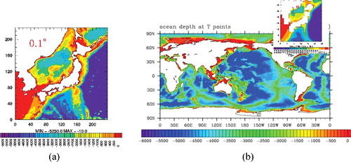
Figure 2(a) shows the bottom topography of the area simulated by ROMS. The 1/10° resolution can adequately represent the coastline and topography around Japan. The ocean around Japan is deep and the area of the continental shelf with a depth of less than 200 m is narrow.

Figure 2. Bottom topography for (a) ROMS for around Japan and (b) POP for the global ocean.

2.1.4. Calculation of concentration of radionuclides

The basic three-dimensional diffusion equation with the decay of radionuclides is used to describe the concentration of radionuclides: (24) $$\begin{array}{ccc}\hfill \frac{\partial C}{\partial t}& =& -L\left(C\right)+K_h(\varphi ,\lambda ,z){\nabla }^{2}C\hfill \\ & & +K_v(\varphi ,\lambda ,z)\frac{{\partial }^{2}C}{\partial z^2}+{\lambda }_{n}C+S,\hfill \end{array}$$(24) where C is the radionuclide concentration (Bq m⁻³); φ, λ, and z are the geographical coordinates (longitude, latitude, and depth, respectively); t is the time (s); K_h and K_v are the horizontal and vertical diffusivities (m² s⁻¹), respectively, λ_n is the decay constant of the radionuclides (s⁻¹), S is the point source to the bottom mesh (Bq m⁻³ s⁻¹). The advection term L(C) is (25) $$\begin{array}{ccc}\hfill L\left(C\right)& =& \frac{1}{acos\varphi }\left[\frac{\partial }{\partial \lambda }\left(uC\right)+\frac{\partial }{\partial \varphi }\left(vcos\varphi C\right)\right]\hfill \\ & & +\frac{\partial }{\partial z}\left(wC\right),\hfill \end{array}$$(25) where a is the radius of the earth, and u, v, and w are the zonal, meridional, and vertical advective velocities (m s⁻¹) of the results of the ocean general circulation model, respectively.

In a previous study [5], equation to describe the concentration of radionuclide included a simple scavenging model (nuclides were removed from the seawater by a phenomenon in which nuclides are adsorbed onto suspended materials in the seawater and settle to the seabed). The scavenging effect is too complex to be represented by this simple model [15]. Here, we ignore the scavenging effect and acquire conservative results because the simulated results in the surface layer are necessary for the dose assessment. A biogeochemical process model might be useful for representing the scavenging effect in future. Decay products (⁹⁰Sr → ⁹⁰Y, ¹³⁷Cs → ¹³⁷Ba_m, and ²⁴¹Pu → ²⁴¹Am) were ignored in this study because they were found not to be dominant for dose assessment in previous studies [5,7]. We ignore the nuclide supplied by the atmospheric weapons tests, nuclear power plant accidents, and release from nuclear facilities. Therefore, boundary conditions of nuclides concentrations were zero.

2.1.5. Assessment of the dose to the public

The internal dose from ingestion of seafood in the area of calculation is calculated according to ICRP Pub. 72 [16], as in previous studies [5]. The external dose equivalent by marine operations was ignored in this study because it is much smaller than the internal one.

The internal exposure route was taken from guidelines for the calculation model for evaluating the dose equivalent around a nuclear power station during normal operation. Internal exposure is evaluated for a maximally exposed reference person by considering daily averaged seafood ingestion. The numerical model and the values for ingested seafood, in which the radionuclides are concentrated, were obtained from the guidelines [17,18].

The equivalent dose to the public is estimated by the radionuclide concentration in the ocean by using the following equation: $$\begin{array}{ccc}& & \left[\mathrm{Equivalent}\mathrm{dose}\mathrm{to}\mathrm{the}\mathrm{public}\left(\mathrm{Bq}\mathrm{yea}{{\mathrm{r}}^{-}}^1\right)\right]\hfill \\ & & =\left[\mathrm{Radionuclide}\mathrm{concentration}\mathrm{in}\mathrm{the}\mathrm{ocean}\left(\mathrm{Bq}{{\mathrm{m}}^{-}}^3\right)\right]\hfill \\ & & \times \left[\mathrm{Dose}\mathrm{factor}\left(\mathrm{Sv}\mathrm{B}{{\mathrm{q}}^{-}}^1\right)\right]\hfill \\ & & \times \left[\mathrm{Concentration}\mathrm{factor}(\left(\mathrm{Bq}{{\mathrm{g}}^{-}}^1\right)/\left(\mathrm{Bq}\mathrm{c}{{\mathrm{m}}^{-}}^3\right))\right]\hfill \\ & & \times \left[\mathrm{Ingestion}\mathrm{rate}\left(\mathrm{g}\mathrm{da}{{\mathrm{y}}^{-}}^1\right)\right]\hfill \end{array}$$

The parameters are summarized in Table 2.

Table 2. Conditions and parameters for estimation of the dose equivalent.

Item		Condition or parameter
Model		ICRP Pub.72
Dose to estimate		Effective dose equivalent for individual
Internal dose	Ingestion of seafood	Consumption (g day^−^1)	Fish	200
			Invertebrate	20
			Seaweed	40
External dose	Working on shipboard	Working period (day year^−^1)		120
	Swimming			4
	Working at beach			20
	Operation of fishery net			80

Simulated radionuclide concentrations varied spatiotemporally by the regional ocean model. We used the maximum concentration in space and time to estimate the conservative dose equivalent.

2.2. Deep sea case

2.2.1. Radionuclide release scenario

The supposed submergence points are along the supposed transport routes from Europe to Japan. The depths of the points are from 1000 m to 3500 m.

The depth of submergence of the package is estimated to be several thousand meters, far from the coast. The package will not retain its integrity because of the high water pressure. In this case, no package is considered. Accordingly, a conservative scenario is assumed as follows:

(1)	The package is submerged on the seabed at a depth of several thousand meters.
(2)	The radioactive materials are exposed to the seawater.
(3)	Nuclides leach directly into the seawater.

2.2.2. Ocean general circulation model for flow field

In this study we use the version of the Los Alamos POP developed for the NCAR Community Climate System Model (CCSM) version 2 [13] as a coarse resolution ocean general circulation model.

The horizontal resolution is 1.125° in longitude and from 0.28° to 0.54° in latitude. There are 40 vertical levels with a minimum spacing of 10 m near the surface, increasing with depth to a maximum spacing of 250 m. This configuration of POP includes the K-Profile Parameterization (KPP) vertical mixing scheme [19], Gent-McWilliams eddy parameterization [20], anisotropic horizontal viscosity [21], and near-surface eddy flux parameterization [22], as the same as a simulation of the global fallout of ¹³⁷Cs due to atmospheric weapons tests [23]. The physical model configurations and parameterizations are summarized in the paper [24]. Figure 2(b) shows the bottom topography for the POP. The average depth of ocean is about 4000 m. Only on the continental shelf is the depth less than 200 m, but that area is quite small. The resolution of the model is lower than the model for the Fukushima accident [11] because this model simulates the annual averaged distribution of radioactive materials for global ocean to estimate dose equivalent for hypothetical accident. The insert in Figure 2(b) shows the bottom topography for the POP around Japan. The resolution of the coastline and topography is not good enough to simulate ocean circulation near the shore around Japan in detail. The surface fluxes are the same as in the near shore case.

2.2.3. Calculation of concentration of radionuclides

The basic three-dimensional diffusion equation with a decay term is employed in the same manner as in the near shore case.

2.2.4. Assessment of the dose to the public

The internal dose from ingestion of seafood in the area of calculation is calculated in the same manner as in the near shore case.

3. Results and discussion

3.1. Near shore case

3.1.1. Release rates of radionuclides

The release rates of radionuclides from the CSD-C and CSD-B packages were estimated by the barrier effect model. The release rates increased with time until the radionuclide concentration saturated within one year. After that, the release rates decreased with time from decay. The time scale for estimation in the near shore case was shorter than the decay time of the target radionuclides in this study. Therefore, the release rates were nearly constant. Tables 3 and 4 summarize the estimated release rates of radionuclides from the CSD-C and CSD-B packages, respectively.

Table 3. Results of release rate estimations from a CSD-C canister.

				Release rate (Bq year^−^1)
				Barrier model	No barrier model
Nuclides	Half-life (year)	Specific activity (Bq g^−^1)	Q (Bq)	Near shore	Deep sea
Sr-90	29	5.06E+12	5.78E+13	1.39E+05	2.25E+11
Tc-99	213,000	6.29E+08	1.19E+10	1.90E+01	4.63E+07
Cs-137	30	3.23E+12	6.46E+13	1.35E+05	2.51E+11
Pu-α			3.30E+12	4.61E+04	3.55E+09
Am-241	432	1.27E+11	4.51E+11	9.36E+03	4.86E+08
Cm-244	18	3.00E+12	2.04E+12	2.23E+05	2.20E+09

Table 4. Results of release rate estimations from a CSD-B canister.

				Release rate (Bq year^−^1)
				Barrier model	No barrier model
Nuclides	Half-life (year)	Specific activity (Bq g^−^1)	Q (Bq)	Near shore	Deep sea
Sr-90	29	5.06E+12	2.48E+13	1.39E+05	1.71E+11
Tc-99	213000	6.29E+08	2.31E+10	1.90E+01	1.59E+08
Cs-137	30	3.23E+12	8.80E+13	1.35E+05	6.06E+11
Pu-238	88	6.34E+11	1.38E+11	4.61E+04	9.50E+08
Pu-239	24065	2.30E+09	4.29E+10	1.68E+02	2.95E+08
Pu-240	6537	8.45E+09	5.39E+10	6.18E+02	3.71E+08
Am-241	432	1.27E+11	9.90E+11	9.36E+03	6.82E+09
Cm-244	18	3.00E+12	4.35E+11	2.23E+05	2.99E+09

3.1.2. Tracer concentration in the ocean

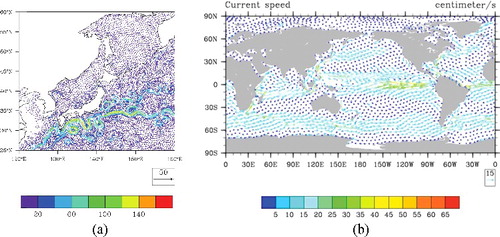
Figure 3(a) shows a snapshot of the current field around Japan. This model can simulate the Kuroshio as western boundary currents. The separation point of the Kuroshio is off the Boso Peninsula, which corresponds to the observed results. Moreover, this model can also simulate the Oyashio current along the Kuril Islands and the Tsugaru current along the coast in the Japan Sea. This eddy resolving model can simulate many of the meso-scale eddies, which play an important role in tracer advection and diffusion.

Figure 3. Ocean current distributions in the surface layer. Vectors show the current speed and direction. Color scale also shows the current speed. (a) ROMS around Japan. For clarity, vectors are only shown over a 1/2° grid. (b) POP for the global ocean. For clarity, vectors are only shown over a 5° grid.

The tracer distribution was simulated for 4 years for the case of continuous release at a rate of 1 unit year⁻¹ from the bottom at six points around Japan at a depth of 200 m for comparison. Tracer advected to the surface layer within a first year. The surface concentration showed seasonal change. The annual cycles for the third and fourth year were quite similar; therefore, the tracer distribution was nearly steady after three years.

Tracer concentration in the surface layer shows the seasonal variation. The variation patterns are similar after second year from the tracer release. Figure 4 shows the maximum monthly mean tracer concentrations in the 0–100 m depth layer during the fourth year off (a) Kyushu in March, (b) Shikoku in March, (c) Hamaoka in May, (d) Wakasa in November, (e) Rokkasho in September and (f) Fukushima in February. Release depths, release points, maximum tracer concentrations, and their points are summarized in Table 5. The tracers advected and diffused by the ocean circulation. Off Kyushu, the tracers were advected along the coast of Kyushu and in the Pacific Ocean by the Kuroshio. Off Shikoku and Hamaoka, the tracers were advected along the course of the Kuroshio. The dilution rate of the tracers was larger than off Kyushu because of the stronger current (Kuroshio). Off Wakasa, the tracers were advected along the course of the Tsushima warm current and the counter-current in the deeper layer. Off Rokkasho and Fukushima, the tracers were advected along the Oyashio. The dilution rate of the tracers was smaller than off Kyushu because of the weaker current (Oyashio). The tracer concentration at the surface was on the order of 10⁻¹⁴ to 10⁻¹³ unit m⁻³. The advection pattern was different for each area, but the differences between the dilution rates were relatively small. Note that these values are conservative because the scavenging effect and decay were ignored in this study.

Figure 4. Monthly averaged surface distributions of tracer concentration (unit m⁻³) by ROMS at 1 unit year⁻¹ release. The X shows the release point and the triangle shows the point of maximum concentration.

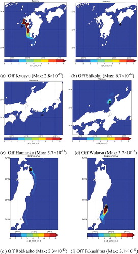
Table 5. Release depths, release points, maximum tracer concentrations, and their points for the near shore cases

	Release	Release point		Point of maximum concentration		Tracer
Case	depth (m)	Latitude	Longitude	Latitude	Longitude	concentration
Hamaoka	200	34.270° N	138.260° E	34.677° N	138.401° E	3.7E-14
Wakasa	200	36.510° N	136.050° E	36.717° N	136.077° E	3.7E-14
Shikoku	200	32.610° N	132.820° E	32.720° N	132.833° E	6.7E-14
Rokkasho	200	40.920° N	141.620° E	40.930° N	141.515° E	2.3E-13
Kyusyu	200	32.380° N	129.260° E	32.782° N	129.792° E	2.8E-13
Fukushima	200	37.310° N	141.470° E	37.211° N	141.456° E	3.1E-13

3.1.3. Radionuclide concentrations in the ocean

Radionuclide concentrations in the ocean (Bq m⁻³) for each release rate of radionuclides (Bq year⁻¹) were estimated from the tracer concentrations (unit m⁻³) with a unit release of tracer (1 unit year⁻¹). The difference of tracer concentrations was one order of magnitude for each submerged point. We selected the maximum concentrations for conservative estimation. The spatiotemporal maximum tracer concentration was 3.1 × 10⁻¹³ unit m⁻³ off Fukushima in the surface layer (0–100 m) with unit release. The spatiotemporal maximum radionuclide concentrations from the CSD-C and CSD-B packages are summarized in Tables 6 and 7, respectively. The results of both the CSD-C and CSD-B are similar due to the barrier effect.

Table 6. Estimated results of radionuclides concentration and dose equivalent for public at the submergence of a CSD-C canister near shore.

	Release rate	Concentration in seawater	Dose equivalent
Nuclides	(Bq year^−^1)	(Bq m^−^3)	(mSv year^−^1)
Sr-90	1.39E+05	4.30E-08	4.60E-12
Tc-99	1.90E+01	5.88E-12	9.07E-17
Cs-137	1.35E+05	4.18E-08	2.61E-13
Pu-α	4.61E+04	1.43E-08	5.35E-11
Am-241	9.36E+03	2.90E-09	4.64E-11
Cm-244	2.23E+05	6.92E-08	6.85E-10
Total			7.90E-10

Table 7. Estimated results of radionuclides concentration and dose equivalent for public at the submergence of a CSD-B canister near shore.

	Release rate	Concentration in seawater	Dose equivalent
Nuclides	(Bq year^−^1)	(Bq m^−^3)	(mSv year^−^1)
Sr-90	1.39E+05	4.30E-08	4.60E-12
Tc-99	1.90E+01	5.88E-12	9.07E-17
Cs-137	1.35E+05	4.18E-08	2.61E-13
Pu-238	4.61E+04	1.43E-08	5.35E-11
Pu-239	1.68E+02	5.21E-11	2.12E-15
Pu-240	6.18E+02	1.92E-10	7.82E-15
Am-241	9.36E+03	2.90E-09	4.64E-11
Cm-244	2.23E+05	6.92E-08	6.85E-10
Total			7.90E-10

Artificial radionuclides (¹³⁷Cs, ⁹⁰Sr, and ^239,240Pu) were introduced to the ocean surface mainly from global fallout originating from atmospheric nuclear weapon tests since 1945. The observed concentrations of artificial nuclides are summarized in a database [25] (and extended). The fallout concentration was high in the early 1960s when atmospheric nuclear weapon tests were being carried out. The observed ¹³⁷Cs, ⁹⁰Sr, and ^239,240Pu concentrations were 20–50, 20—50, and 0.5–0.8 Bq m⁻³ in the North Pacific in the early 1960s, respectively. They reduced to 1–4, 1—4, and 0.01–0.4 Bq m⁻³ by the 1990s, respectively.

The maximum observed ¹³⁷Cs concentration in the Irish Sea was 2.0 × 10⁵ Bq m⁻³ in 1974 due to the release from the BNFL nuclear fuel reprocessing plant at Sellafield, UK. The observed maximum concentration of ¹³⁷Cs from the Fukushima Daiichi Nuclear Power Plant accident was 6.8 × 10⁷ Bq m⁻³ [9]. The estimated radionuclide concentrations in this study are smaller than the values observed in the past.

3.1.4. Dose equivalent to the public

We estimated the equivalent dose to the public from the radionuclide concentrations in the ocean due to the hypothetical submergence of either a CSD-C or CSD-B package within one canister. The total dose equivalents from the CSD-C and CSD-B packages were 7.9 × 10⁻¹⁰ and 7.9 × 10⁻¹⁰ mSv year⁻¹, respectively (Tables 6 and 7). ²⁴⁴Cm was the dominant radionuclide for both estimations. Even if barrier effect is not considered for more conservative estimations, the total dose equivalents from the CSD-C and CSD-B packages were 2.1 × 10⁻⁵ and 5.1 × 10⁻⁵ mSv year⁻¹, respectively. The dose equivalent by fallout was estimate to be 2.4 × 10⁻³ mSv year⁻¹ in the 1960s and 2.3 × 10⁻⁴ mSv year⁻¹ in the 1990s from the averaged background concentrations of ¹³⁷Cs, ⁹⁰Sr, and ^239,240Pu. The estimated dose equivalents in this study are much smaller than those due to global fallout and natural sources. The estimated dose equivalents are also much smaller than the ICRP recommendation (1 mSv year⁻¹).

3.2. Deep sea case

3.2.1. Release rates of radionuclides

The release rate is equal to the leaching rate because no barrier effect was employed in the deep sea submergence case. The release rate decreased with time by decay. Tables 3 and 4 summarize the estimate maximum release rates of radionuclides from CSD-C and CSD-B packages, respectively.

3.2.2. Tracer concentration in the ocean

Figure 3(b) shows the global annual mean current field. This model can simulate a typical ocean current, such as the Kuroshio or Gulf Stream, as western boundary currents. The Equatorial Current and the Antarctic Circumpolar Current are also represented. The separation point of the Kuroshio was north off the Boso Peninsula because this coarse resolution model cannot simulate western boundary currents correctly. In addition, the maximum current speed of the Kuroshio was smaller than the one simulated by the eddy resolving model, ROMS. This coarse resolution model cannot represent meso-scale eddies. The effects of meso-scale eddies on tracer diffusion is simulated by the Gent-McWilliams eddy parameterization [19]. The long-term tracer simulation of the eddy resolving model in the global ocean is difficult due to present limits on computational resources. The coarse resolution model with eddy parameterization is still useful for long-term global tracer simulation.

The tracer distribution was simulated for 100 years for the case of continuous release at the rate of 1 unit year⁻¹ from the bottom at six points all over the world for comparison.

Figure 5 shows the maximum annual mean tracer concentration for (a) near Japan, (b) Solomon Islands, (c) Tasman Sea, (d) Drake Passage, (e) Atlantic Ocean, and (f) Kerguelen Islands in the surface layer (0–100 m depth). Release depths, release points, maximum tracer concentrations, and their points are summarized in Table 8.

Figure 5. Annual averaged surface distributions of tracer concentration (unit m⁻³) by POP at 1 unit year⁻¹ release. The X shows the release point and the circle with cross shows the point of maximum concentration.

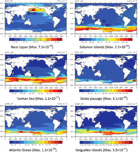
Table 8. Release depths, release points, maximum tracer concentrations, and their points for the deep sea cases

		Release point		Point of maximum concentration
Case	Release depth (m)	Latidude	Longitude	Latidude	Longitude	Tracer concentration
Near Japan	2250	31.419° N	139.433° E	50.985° N	165.213° E	7.5E-19
Solomon islands	2250	15.7161° S	168.688° E	59.9886° S	73.063° E	2.2E-18
Tasman Sea	1250	32.2081° S	161.938° E	59.9886° S	71.938° E	1.1E-17
Drake passage	3500	57.8517° S	66.438° W	61.5913° S	12.438° W	3.1E-18
Atlantic Ocean	3000	2.525° N	30.438° W	62.1255° S	95.563° E	1.1E-18
Kerguelen islands	1020	51.4409° S	73.063° E	59.9886° S	147.312° E	3.5E-17

The order of magnitude of the tracer concentration at the surface was in the range of 10⁻¹⁹ to 10⁻¹⁷ unit m⁻³. The advection pattern was different for each area, but the differences between the dilution rates were relatively small. Note that these values are conservative because both the scavenging effect and decay were ignored in this study.

The simulated surface concentration was maximum in the subarctic zone for submergence near Japan due to northeast advection. In other cases, the simulated surface concentration was maximum in the Southern Ocean due to the deep current and upwelling of the circumpolar current near the Kerguelen Islands. The radionuclide concentration in the surface layer reached a steady state during 100 years.

3.2.3. Radionuclide concentrations in the ocean

The radionuclide concentrations in the ocean (Bq m⁻³) with each release rate of radionuclides (Bq year⁻¹) were estimated from tracer concentrations (unit m⁻³) with unit releases of tracer (1 unit year⁻¹). The difference of tracer concentrations was two orders of magnitude for each submerged point. We selected the maximum concentrations for conservative estimation. The spatiotemporal maximum tracer concentration was 3.5 × 10⁻¹⁷ unit m⁻³ at Kerguelen Islands in the surface layer with unit release. The simulated concentration in the surface layer reached a maximum value 100 years after release. The spatiotemporal maximum radionuclide concentrations from CSD-C and CSD-B are summarized in Tables 9 and 10, respectively.

Table 9. Estimated radionuclide concentrations and dose equivalents from the submergence of a CSD-C canister in deep sea.

	Release rate	Concentration in seawater	Dose equivalent
Nuclides	(Bq year^−1)	(Bq m^−3)	(mSv year^−1)
Sr-90	2.25E+11	7.87E-06	8.42E-10
Tc-99	4.63E+07	1.62E-09	2.50E-14
Cs-137	2.51E+11	8.79E-06	5.50E-11
Pu-α	3.55E+09	1.24E-07	4.66E-10
Am-241	4.86E+08	1.70E-08	2.72E-10
Cm-244	2.20E+09	7.69E-08	7.61E-10
Total			2.40E-09

Table 10. Estimated radionuclide concentrations and dose equivalents from the submergence of a CSD-B canister in deep sea.

	Release rate	Concentration in seawater	Dose equivalent
Nuclides	(Bq year^−^1)	(Bq m^−^3)	(mSv year^−^1)
Sr-90	1.71E+11	5.98E-06	6.39E-10
Tc-99	1.59E+08	5.57E-09	8.58E-14
Cs-137	6.06E+11	2.12E-05	1.33E-10
Pu-238	9.50E+08	3.32E-08	1.25E-10
Pu-239	2.95E+08	1.03E-08	4.22E-13
Pu-240	3.71E+08	1.30E-08	5.30E-13
Am-241	6.82E+09	2.39E-07	3.82E-09
Cm-244	2.99E+09	1.05E-07	1.04E-09
Total			5.75E-09

Dilution rates for the deep sea case were larger than those for the near shore case. On the other hand, the release rates for the deep sea case were larger than those for the near shore case. As a result, the estimated radionuclide concentrations for the deep sea case were similar to those for the near shore case. The estimated radionuclide concentrations in this study are smaller than values observed in the past.

3.2.4. Dose equivalent to the public

From the radionuclide concentrations in the ocean, we estimated the equivalent dose to the public from the hypothetical submergence of either a CSD-C or CSD-B package within one canister. The total dose equivalents from CSD-C and CSD-B were 2.4 × 10⁻⁹ and 5.8 × 10⁻⁹ mSv year⁻¹, respectively (Tables 9 and 10). ⁹⁰Sr and ²⁴¹Am are the dominant radionuclides for CSD-C and CSD-B estimations, respectively. The estimated dose equivalents are much smaller than both those experienced in the past and the ICRP recommendation (1 mSv year⁻¹).

4. Conclusions

The estimated dose equivalents from the hypothetical submergence of CSD-C and CSD-B packages are summarized in Table 11 along with the results for spent fuel, high level waste, and MOX fuel packages. CSD-C and CSD-B packages contain 36 and 10 canisters, respectively. The estimated dose equivalents from CSD-C and CSD-B packages were 2.8 × 10⁻⁸ and 7.9 × 10⁻⁹ mSv year⁻¹, respectively, for the near shore case. These doses are 1000–100,000 times smaller than that from one of the Type B packages (spent fuel, high level waste, and MOX fuel) for the near shore case. The estimated dose equivalents from CSD-C and CSD-B packages were 8.6 × 10⁻⁸ and 5.8 × 10⁻⁸ mSv year⁻¹, respectively, for the deep sea case. These doses are 1000 times smaller than those for spent fuel and high level waste and similar to that of MOX fuel for the deep sea case. The estimated dose equivalents are much smaller than past exposures and the ICRP recommendation[26].

Table 11. Summary of the estimated dose equivalents from one package.

	Transport package	Main nuclide	Dose equivalent (mSv year^−^1)
Near shore	Spent fuel	^244Cm	5.0 × 10^−4
	High level waste	^244Cm	5.0 × 10^−4
	MOX fuel	^238Pu	5.0 × 10^−6
	CSD-C	^244Cm	2.8 × 10^−^8
	CSD-B	^244Cm	7.9 × 10^−^9
Deep sea	High level waste	^244Cm	1.0 × 10^−5
	MOX fuel	^238Pu	1.0 × 10^−9
	CSD-C	^241Am	8.6 × 10^−^8
	CSD-B	^90Sr	5.8 × 10^−^8
Fallout in the ocean	1960s	^137Cs, ^90Sr	2.4 × 10^−3
	1990s	^239,240Pu	2.3 × 10^−4
Natural radiation	Total		2.4
	Internal dose from food		3.4 × 10^−1
ICRP recommendation			1.0

CSD-C 36 canisters/package.

CSD-B 10 canisters/package.

Bold values show the results in this study. Other values show the results in the previous study [27].

Disclosure statement

No potential conflict of interest was reported by the authors.

References

- Heaberlin SW, Baker DA, Beyer CE, et al. Consequences of postulated losses of LWR spent fuel and plutonium shipping packages at sea, Rep. BNWL-2093. Richland (WA): Battelle Pacific Northwest Labs; 1977.
- Nagakura T, Maki T, Tanaka N. Safety evaluation on transport of fuel at sea and test program on full scale cask in Japan. Proceedings of PATRAM'78; 1978 May; Albuquerque (NM): Sandia Laboratories. p. 143–149.
- IAEA. Advisory material for the IAEA regulations for the safe transport of radioactive material safety guide, Safety Standards Series No. TS-G-1.1 (Rev.1);. 2008, Vienna: International Atomic Energy Agency.
- Watabe N, Kohno Y, Tsumune D, et al. An environmental impact assessment for sea transport of high level radioactive waste. Int J Radioact Mater Transport. 1996;7:117–127.
- Tsumune D, Saegusa T, Suzuki H, et al. Watabe, estimated radiation dose from a MOX fuel shipping package that is hypothetically submerged into Sea. Int J Radioact Mater Transport. 2000;11:239–253.
- IAEA, Accident severity at Sea during transport of radioactive material. IAEA TECDOC 1231; 2000; 180 pp.
- Tsumune D, Saegusa T, Suzuki H, et al. Dose assessment for the public due to packages shipping radioactive materials hypothetically sunk on a continental shelf. Int J Radioact Mater Transport. 2000;11:317–328.
- Tsumune D, Saegusa T, Itoh C. Assessment for radiological impact of irradiated nuclear fuel package sunk in marine environment. J Pack Transport Storage Secur Radioact Mater. 2007;18:123–129.
- Tsumune D, Tsubono T, Aoyama M, et al. Distribution of oceanic 137Cs from the Fukushima Daiichi nuclear power plant simulated numerically by a regional ocean model’. J Environ Radioact. 2012;111:100–108. DOI:10.1016/j.jenvrad.2011.10.007
- Tsumune D, Tsubono T, Aoyama M, et al. One-year, regional-scale simulation of 137Cs radioactivity in the ocean following the Fukushima Dai-ichi nuclear power plant accident. Biogeosciences. 2013;10:5601–5617. DOI:10.5194/bg-10-5601-2013
- Tsubono T, Misumi K, Tsumune D, et al. Evaluation of radioactive cesium impact from atmospheric deposition and direct release fluxes into the North Pacific from the Fukushima Daiichi nuclear power plant. Deep Sea Res Pt I. 2016;115:10–21.
- Shchepetkin AF, McWilliams JC. The regional ocean modeling system (ROMS): a split-explicit, free-surface, topography following coordinates oceanic model. Ocean Model. 2005;9:347–404.
- Kiehl JT, Gent PR. The community climate system model, version 2. J Climate. 2004;17:3666–3682.
- Large WG, Yeager SG. Diurnal to decadal global forcing for ocean and sea-ice models: the data sets and flux climatologies. NCAR Technical Note NCAR/TN-460+STR, National Center for Atmospheric Research (NCAR), 2004; p. 111.
- Misumi K, Lindsay K, Moore JK, et al. Humic substances may control dissolved iron distributions in the global ocean: implications from numerical simulations. Global Biogeochem Cycles 2013;27:450–462. DOI:10.1002/gbc.20039
- ICRP. Age-dependent doses to the members of the public from intake of radionuclides – Part 5 compilation of ingestion and inhalation coefficients, ICRP Publication 72. Ann. ICRP 1995; p. 26.
- Nuclear Safety Committee. The assessment guideline for the target of dose equivalent around the light water reactor. 1976, revised 1989. Japanese. Japan: Nuclear Safety Committee.
- Nuclear Safety Committee. The assessment of radiation exposure to public at the light water reactor power station in safety examination, 1989. Japanese, Japan: Nuclear Safety Committee.
- Large WG, McWilliams JC, Doney SC. Ocean vertical mixing: a review and a model with a nonlocal boundary layer parameterization, Rev Geophys. 1994;32:363–403.
- Gent PR, McWilliams JC. Isopycnal mixing in ocean circulation models. J Phys Oceanogr. 1990;20:150–155.
- Smith RD, McWilliams JC. Anisotropic horizontal viscosity for ocean models. Ocean Model. 2003;5:12–156.
- Danabasoglu G, Ferrari R, McWilliams JC. Sensitivity of an ocean general circulation model to a parameterization of near-surface eddy fluxes. J Climate. 2008;21:1192–1208.
- Tsumune D, Aoyama M, Hirose K, et al. Transport of 137Cs to the southern hemisphere in an ocean general circulation model. Prog Oceanogr. 2011;89:38–48. DOI:10.1016/j.pocean.2010.12.006
- Yeager SG, Jochum M. The connection between labrador Sea buoyancy loss, deep western boundary current strength, and Gulf Stream path in an ocean circulation model. Ocean Model. 2009;30:207–224.
- Aoyama M, Hirose K. Artificial radionuclides database in the pacific ocean: ham database’. Scientific World J. 2004;4:200–215.
- ICRP, The 2007 Recommendation of International Commission on Radiological Protection. ICRP Publication 103. Ann. ICRP. 2007, p. 34.
- Tsumune D, Tsubono T,Saegusa T, Radiological impact assessment at the hypothetical release from submerged transport package of high level radioactive materials, CRIEPI Report, V09041, 2010, p. 20, Japanese.