Research on the design method of highly loaded helium compressor based on the physical properties

ABSTRACT

A highly loaded design method of helium compressor is presented in this paper. First, particular loss prediction models based on corrections of isentropic index and velocity triangle are deduced for highly loaded helium compressor. Then the influence of design parameters such as reaction, flow coefficient and load coefficient on aerodynamic loss of highly loaded helium compressor is analyzed in detail with the loss models. The design principles are also discussed. A highly loaded helium compressor design study is carried out based on a 300-MW high-temperature gas-cooled reactor (HTGR) helium multistage compressor to validate the method. The results indicate that the 16-stage helium low-pressure compressor of the 300-MW HTGR can be reduced to a 3-stage compressor by the proposed highly loaded design method at the same tip tangential velocity. The isentropic efficiency could be as high as 90% under design condition.

KEYWORDS:

• HTGR
• helium compressor
• highly loaded
• loss prediction model

1. Introduction

High-temperature gas-cooled reactor (HTGR) is a typical fourth-generation nuclear reactor with excellent characteristics of safety, economy and environmental protection [1–5]. By using helium as the working fluid, the closed Brayton cycle system can provide a turbine inlet temperature over 900 °C. Compared with secondary circuit steam cycle, the cycle efficiency of the helium direct cycle can be increased by 50%. Helium compressor is the key component of the closed Brayton cycle power conversion unit of HTGR. Helium is difficult to be compressed because its thermodynamic properties are quite different from those of air (specific heat of helium is 5 times that of air; isentropic index of helium is 1.2 times that of air; sound velocity of helium is 3 times that of air, etc.), which results in huge increase in the stage number of the helium compressor, if the conventional design method is applied. The increase in the stage number increases the compressor length as well as the number of blades. The longer rotor could cause rotor dynamic problems.

In 1980s, EVO 50-MW [6] nuclear reactor unit (the biggest helium turbine device at that time) was deployed in Germany, whose total stage number of low-pressure compressor and high-pressure compressor was 25. The unit operated for 24,000 h; however, its maximum power was only 30.5 MW. Analysis showed that the main reason of power reduction was the incorrect prediction of compressor efficiency. An improved design containing a 41-stage compressor was put forward later. JAERI published the detailed aerodynamic design of a helium compressor and the design was validated by experiments on some helium compressor stages of the 600-MW and 300-MW HTGR power plant [7–8]. To fulfill the target that efficiency should not be lower than 90%; although some advanced design methods such as Controlled Diffusion Airfoils (CDA) airfoil and end-bending were adopted, it still took 31 stages and 35 stages, which were much longer than those of the traditional air compressor, to achieve 3.13 and 2.46 pressure ratio, respectively.

The mismatch between the thermodynamic properties of helium and traditional air compressor design method is the main reason why helium is hard to be compressed. The general parameter selection principle results in a lower flow Mach number in the helium compressor. The helium works like flow incompressible fluids.

The new compressor design method focusing on characteristics of helium was put forward by Russian researchers aiming at closed cycle system first [9]. The authors suggested to increase Euler work by increasing flow coefficient and then to compare and analyze the effects of flow coefficient on both air and helium compressor target efficiency. Unfortunately, further discussion and verification is interrupted for this kind of highly loaded helium compressor. The velocity triangle of a highly loaded helium compressor elementary stage was analyzed by Long et al in detail [10]. The design characteristics (high reaction, big flow deflection and minus prewhirl) were found and the flow field characteristics of the compressor were also analyzed. Later then based on highly loaded design method, suitable airfoil and twist principle of highly loaded helium compressor were researched by Ke [11–12]. Taking JAEA 300-MW low-pressure compressor as a target, a stage design validation was carried out to achieve the same compression ratio of 16 stages with only 6 stages. In 2015, the blade surface boundary layer growth regularity of the highly loaded helium compressor was analyzed and researched by Jiang [13].

Some profitable and innovative works on the design theory of highly loaded helium compressor are studied by the researchers mentioned earlier. However, a quantitative relation between thermodynamic properties and flow losses is not established. Therefore, assessment criteria are lacking for design parameter selection principles and confirmation of maximum load of highly loaded helium compressor, which means that it is unable to predict loss accurately. Besides, the elementary stage velocity triangle of the compressor is changed radically by highly loaded design, meaning that it is unpractical to use the existing loss model to predict losses of highly loaded helium compressor. Meanwhile, some flow characteristics like stall margin and surge margin are changed. These problems limit the improvement and application of highly loaded helium compressor.

Research on effects of helium thermodynamic properties on compressor losses is seldom. Roberto [14–15] did a persistence work on the relation of loss between helium and air by using dimensional analysis to construct an efficiency relationship between helium and air under different circumstances. However, the problem about quantitative prediction of helium compressor performance remains unsolved, especially that of highly loaded helium compressor. Obviously, restudying on the loss model of highly loaded helium compressor is uneconomical and infeasible. So, the purpose of this paper is to find out that how to establish an effective loss prediction strategy to obtain the basic design law of highly loaded helium compressor and markedly increase single-stage load on the basis of inheriting air compressor design experience.

In this paper, a design method and the optimal parameter selection principles of the highly loaded helium compressor are presented. The Smith chart of the highly loaded helium compressor is investigated and compared with that of air compressor. A design practice of the highly loaded helium compressor is carried out by using the above proposed method. Finally the designed helium compressors are validated with computational fluid dynamics (CFD) numerical simulation.

2. The availability of the new velocity triangle

Helium is considered as an ideal coolant for HTGR due to the thermodynamic properties. The isentropic index and the specific heat of helium are almost not changed with the temperature. The thermal conductivity of helium is two times that of air and the specific heat is five times that of air. However, as the working fluid of power conversion unit of HTGR, it brings many difficulties to the design of the compressor. The specific heat of helium is bigger than that of air, so the helium compressor has a small single-stage pressure ratio. In order to resolve these difficulties, highly loaded design method is investigated.

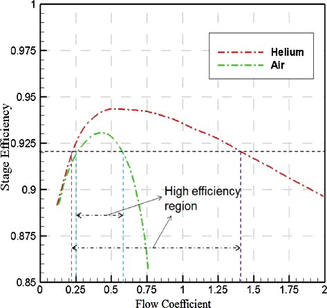
The relationship between stage efficiency and flow coefficient has been given in Figure 1. When the flow coefficient is less than 0.25, there is no difference between air and helium. If the flow coefficient is larger than 0.25, the helium compressor has higher efficiency than air compressor, which means the higher efficiency range of helium compressor is three times that of air compressor. So, high flow coefficient is desirable for the design of helium compressor.

Figure 1. Relation of stage efficiency and flow coefficient under the condition of 0.5 reactions for helium and air.

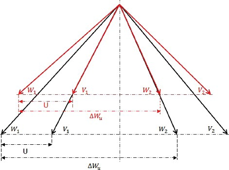
The velocity vectors and associated velocity diagram for a typical highly loaded axial-flow helium compressor stage are shown in Figure 2. The enthalpy rise along the streamline is given as follows: (1) $$\begin{array}{c}\hfill \Delta h=(W_{1u}+W_{2u})\times U\end{array}$$(1)

Figure 2. Velocity diagram in highly loaded helium compressor.

Based on the characteristics of high sound speed of helium, the velocity triangle of highly loaded compressor increases the torsional velocity greatly by increasing both the axial velocity and a negative prewhirl. Therefore, if the circumferential velocity is unchanged, the stage loading will increase greatly.

When increasing the backpressure, the specific power and adverse pressure gradient of compressor designed by general velocity triangle increase as well. Therefore, high load coefficient makes that kind of compressor unstable. By using new velocity triangle, the specific power and adverse pressure gradient of highly loaded helium compressor decrease in the same change, which means that the highly loaded helium compressor works stable when the backpressure is increased, as shown in Figure 3.

Figure 3. Velocity triangle of highly loaded helium compressor.

3. Improvement of the blade-profile loss model

Because no experimental data of highly loaded helium compressor is available, the total pressure loss model of highly loaded helium compressor has to be derived from those of air compressor. The prototype air compressor loss model is revised considering the thermodynamic helium properties correction of helium compressor first. Then the calculation method of the blade-profile pressure loss coefficient has also been changed according to the difference between the velocity triangles.

3.1. Deduction of the loss model

3.1.1. Basic loss model

Lieblein [16,17] defined the blade-profile pressure loss coefficient for air compressor as: (2) $$\begin{array}{ccc}\hfill Y_p& =& 2\left(\frac{{\theta }_2}{C}\right)\times \frac{\sigma }{cos{\phi }_2}\times {\left(\frac{cos{\phi }_1}{cos{\phi }_2}\right)}^2\times \left(\frac{2H_{TE}}{3H_{TE}-1}\right)\hfill \\ & & \times {\left[1-\left(\frac{{\theta }_2}{C}\right)\frac{\sigma H_{TE}}{cos{\phi }_2}\right]}^{-3}\hfill \end{array}$$(2)

Based on the experimental data of Koch and Smith [18], the boundary-layer momentum thickness at the compressor cascade outlet is expressed as: (3) $$\begin{array}{ccc}\hfill \left(\frac{{\theta }_2}{C}\right)& =& (2.644\times {10}^{-3}\times D^{*}-1.519\times {10}^{-4}\hfill \\ & & +\frac{6.713\times {10}^{-3}}{2.6-D^{*}})\times {\zeta }_H\times {\zeta }_{Re}\times {\zeta }_{Ma}\hfill \end{array}$$(3)

The boundary layer thickness at trailing edge is correlated as: (4) $$\begin{array}{ccc}\hfill H_{TE}^0& =& (0.91+0.35\times D^{*})\hfill \\ & & \times \left[1+0.48\times {\left(D^{*}-1\right)}^4+0.21\times {(D^{*}-1)}^6\right]\hfill \end{array}$$(4)

A value of H⁰_TE = 2.7209 is used when D^* > 2.0. (5) $$\begin{array}{c}\hfill H_{TE}=H_{TE}^0\times {\xi }_H\times {\xi }_{Re}\times {\xi }_{Ma}\end{array}$$(5)

The diffusion ratio D* is defined as: (6) $$\begin{array}{c}\hfill D^{*}=\frac{W_1}{W_2}+\frac{\Delta W_u}{2\sigma W_2}\end{array}$$(6)

For the velocity triangle of highly loaded compressor: (7) $$\begin{array}{c}\hfill D^{*}=\frac{cos{\phi }_2}{cos{\phi }_1}+\frac{cos{\phi }_2}{2\sigma }(tan{\phi }_1+tan{\phi }_2)\end{array}$$(7)

The correction factors were determined by charts that were developed by Koch and Smith [18] .The correction factor for the flow area contraction is given by: (8) $$\begin{array}{c}\hfill {\zeta }_H=0.53\frac{H_1}{H_2}+0.47\end{array}$$(8) (9) $$\begin{array}{c}\hfill {\xi }_H=1.0+\left(\frac{H_1}{H_2}-1.0\right)\times \left(0.0026\times D^{*8}-0.024\right)\end{array}$$(9)

The friction losses that are controlled by the surface roughness and Reynolds correction factor may be expressed as: (10) $$\begin{array}{c}\hfill {\zeta }_{Re}=\left\{\begin{array}{c}{\left({\displaystyle \frac{{10}^6}{R{e}_c}}\right)}^{0.166},\mathrm{for}R{e}_c\ge 2\times {10}^5,\hfill \\ 1.30626\times {\left({\displaystyle \frac{2\times {10}^5}{R{e}_c}}\right)}^{0.5},\mathrm{for}R{e}_c<2\times {10}^5.\hfill \end{array}\right.\end{array}$$(10) (11) $$\begin{array}{c}\hfill {\xi }_{Re}={\left(\frac{{10}^6}{R{e}_c}\right)}^{0.06}\end{array}$$(11)

The correction factor for the inlet Mach number is accurately fitted by: (12) $$\begin{array}{c}\hfill {\zeta }_{Ma}=1.0+\left[0.11757-D^{*}\times 0.16983\right]\times M{a}_1^n\end{array}$$(12) (13) $$\begin{array}{c}\hfill n=2.853+D^{*}\times (0.19477\times D^{*}-0.97747)\end{array}$$(13) (14) $$\begin{array}{ccc}\hfill {\xi }_{Ma}& =& 1.0+\left[1.0725+D^{*}\right.\hfill \\ & & \times \left.\left(-0.8671+0.18043\times D^{*}\right)\right]\times M{a}_1^{1.8}\hfill \end{array}$$(14)

The secondary flow loss coefficient is given by the correlation proposed by Howell [19] as: (15) $$\begin{array}{c}\hfill Y_{sec}=0.018\times \sigma \times \frac{{cos}^2\left({\phi }_1\right)}{{cos}^3\left({\phi }_m\right)}{C}_L^2\end{array}$$(15)

Based on a modified Howell's model [19], Aungier [20] developed the following expression for calculating the end wall loss coefficient as: (16) $$\begin{array}{c}\hfill Y_{EW}=0.0146\times \frac{C}{H}\times {\left(\frac{cos{\phi }_1}{cos{\phi }_2}\right)}^2\end{array}$$(16)

The tip leakage loss factor Y_tip [21] is calculated as: (17) $$\begin{array}{c}\hfill Y_{\mathrm{tip}}=2K_E\sigma \frac{\tau }{H}{C}_D\frac{{cos}^2\left({\phi }_1\right)}{{cos}^3\left({\phi }_m\right)}{C}_L^{1.5}\end{array}$$(17)

The theoretical compressor blade lift coefficient C_L is (18) $$\begin{array}{c}\hfill C_L=\frac{2}{\sigma }\times cos{\phi }_m\times (tan{\phi }_1+tan{\phi }_2)\end{array}$$(18)

The mean velocity vector angle is given by: (19) $$\begin{array}{c}\hfill tan{\phi }_m=0.5\times (tan{\phi }_1+tan{\phi }_2)\end{array}$$(19)

where K_E = 0.566 for a front or aft-loaded blade and K_E = 0.5 for a mid-loaded blade; C_D is a discharge coefficient.

3.1.2. Correction for the loss model

The total pressure loss coefficient in the general compressor cascade is expressed as: (20) $$\begin{array}{c}\hfill Y={\zeta }_n\times {\zeta }_l\times Y_P+Y_{sec}+Y_{tip}+Y_{EW}\end{array}$$(20) where ζ_n is the correction factor based on the nature of helium; ζ_l is the correction factor to consider the higher load of helium compressor.

The compressor channel pressure loss is mainly determined by the viscosity μ, average velocity W, density ρ, blade height H and chord C.

By dimensional analysis: (21) $$\begin{array}{c}\hfill \frac{\Delta p_c}{C}//\mu ,\bar{W},\rho ,H\end{array}$$(21)

Buckingham's π theorem indicates that (22) $$\begin{array}{c}\hfill \frac{\Delta P_{C}H}{C\rho \overline{W^2}}//Re\end{array}$$(22)

Then (23) $$\begin{array}{c}\hfill \Delta p_C=\frac{C}{H}\rho \frac{\overline{W^2}}{2}\lambda \end{array}$$(23)

Thus, the correction factor ζ can be derived that when the two kinds of fluids flow in the same flow channel, the ratio of total pressures through the same compressor channel is (24) $$\begin{array}{c}\hfill {\zeta }_n=\frac{Y_A}{Y_B}=\frac{\frac{{\lambda }_A\overline{{\rho }_A}\overline{W_A^2}}{{\rho }_{A1}{W}_{A1}^2}}{\frac{{\lambda }_B\overline{{\rho }_B}\overline{W_B^2}}{{\rho }_{B1}{W}_{B1}^2}}=\frac{\left(\frac{{\rho }_{A1}{W}_{A1}^2}{{\rho }_{A1}{W}_{A1}^2}+\frac{{\rho }_{A2}{W}_{A2}^2}{{\rho }_{A1}{W}_{A1}^2}\right){\lambda }_A}{\left(\frac{{\rho }_{B1}{W}_{B1}^2}{{\rho }_{B1}{W}_{B1}^2}+\frac{{\rho }_{B2}{W}_{B2}^2}{{\rho }_{B1}{W}_{B1}^2}\right){\lambda }_B}\end{array}$$(24)

Applying conservation of mass across the compressor channel: (25) $$\begin{array}{c}\hfill {\rho }_{X1}{A}_{X1}{W}_{X1}={\rho }_{X2}{A}_{X2}{W}_{X2}\end{array}$$(25) (26) $$\begin{array}{c}\hfill \frac{{\rho }_{X2}}{{\rho }_{X1}}\approx {\left(\frac{P_{X02}}{P_{X01}}\right)}^{\frac{1}{k_x}}\end{array}$$(26)

Then (27) $$\begin{array}{c}\hfill {\zeta }_n=\frac{\left(1+{\pi }^{-2-\frac{1}{{}_{k_A}}}\right){\lambda }_A}{\left(1+{\pi }^{-2-\frac{1}{k_B}}\right){\lambda }_B}\end{array}$$(27)

where π is the pressure ratio.

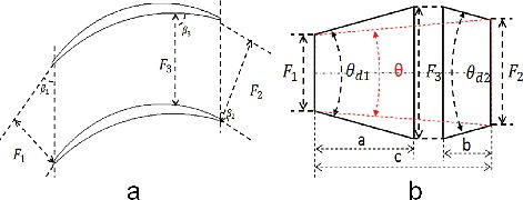
As shown in Figure 4, the highly loaded helium compressor cascade passage is divided into two sections, a (divergent section) and b (contraction section).

Figure 4. Highly loaded helium compressor cascade channel.

ζ_lcan be defined as: (28) $$\begin{array}{c}\hfill {\zeta }_l=\frac{\Delta P_a+\Delta P_b}{\Delta P_c}\end{array}$$(28)

Based on the local loss calculation formula of conical diffuser and conical nozzle ΔP_X can be written as: (29) $$\begin{array}{c}\hfill \Delta P_X=({\varsigma }_X+1)\frac{X}{d}\rho \frac{\overline{W^2}}{2}\lambda \end{array}$$(29)

For conical diffuser, ς_Xcan be written as: (30) $$\begin{array}{c}\hfill {\varsigma }_a=\frac{2.6sin({\theta }_{d1}/2)\left[1-{\left(F_1/F_3\right)}^2\right]}{{\left(F_1/F_3\right)}^4}\end{array}$$(30) (31) $$\begin{array}{c}\hfill {\varsigma }_c=\frac{2.6sin(\theta /2)\left[1-{\left(F_1/F_2\right)}^2\right]}{{\left(F_1/F_2\right)}^4}\end{array}$$(31)

For conical nozzle, ς_X can be written as: (32) $$\begin{array}{c}\hfill {\varsigma }_b=\frac{0.8sin({\theta }_{d2}/2)\left[1-{\left(F_2/F_3\right)}^2\right]}{{\left(F_2/F_3\right)}^4}\end{array}$$(32) where (33) $$\begin{array}{c}\hfill F_3=d-m\end{array}$$(33) (34) $$\begin{array}{c}\hfill F_1=dsin\left({\beta }_1\right)-{\mathrm{r}}_{\mathrm{L}}\end{array}$$(34) (35) $$\begin{array}{c}\hfill F_2=dsin\left(180-{\beta }_2\right)=dsin\left({\beta }_2\right)-{\mathrm{r}}_{\mathrm{T}}\end{array}$$(35)

Diffusion angle can be written as: (36) $$\begin{array}{c}\hfill {\theta }_{d1}=\frac{d(cos\left({\beta }_3\right)-cos\left({\beta }_1\right))}{a}\end{array}$$(36) (37) $$\begin{array}{c}\hfill {\theta }_{d2}=\frac{d(cos\left({\beta }_3\right)-cos\left({\beta }_2\right))}{b}\end{array}$$(37) (38) $$\begin{array}{c}\hfill \theta =\frac{d(cos\left({\beta }_2\right)-cos\left({\beta }_1\right))}{c}\end{array}$$(38)

Then (39) $$\begin{array}{c}\hfill {\zeta }_l=\frac{({\varsigma }_a+1)a+({\varsigma }_b+1)b}{({\varsigma }_c+1)c}\end{array}$$(39) where (40) $$\begin{array}{c}\hfill a+b=c\end{array}$$(40) (41) $$\begin{array}{c}\hfill \frac{b}{a}\approx \frac{{\beta }_2}{{\beta }_1}\end{array}$$(41)

When θ is small, sin(θ) ≈ θ. Then equations can be written as: (42) $$\begin{array}{c}\hfill {\zeta }_l=\frac{\frac{{\beta }_1}{{\beta }_2+{\beta }_1}{\varsigma }_a+\frac{{\beta }_2}{{\beta }_2+{\beta }_1}{\varsigma }_b+1}{{\varsigma }_c+1}\end{array}$$(42)

3.1.3. The total-to-total efficiency

The efficiency of the compressor stage can therefore be written as [22]: (43) $$\begin{array}{c}\hfill \eta =1-\frac{T_{03}\Delta s_{\mathrm{stage}}}{h_{03}-h_{01}}\end{array}$$(43)

If we take the process of helium passing through the rotor as an ideal process at constant relative stagnation enthalpy, h_01,rel, the second law of thermodynamics, Tds = dh − dp/ρ, can be written as: (44) $$\begin{array}{c}\hfill T_{01,\mathrm{rel}}\Delta s_{\mathrm{rotor}}\approx \frac{\Delta P_{0,\mathrm{rotor}}}{{\rho }_{01,\mathrm{rel}}}\end{array}$$(44)

where (45) $$\begin{array}{c}\hfill \Delta P_{0,\mathrm{rotor}}=\Delta P_{01,\mathrm{rel}}-\Delta P_{02,\mathrm{rel}}\end{array}$$(45)

AsP = ρRT, this can be written as: (46) $$\begin{array}{c}\hfill \Delta s_{\mathrm{rotor}}\approx \frac{R\Delta P_{0,\mathrm{rotor}}}{P_{01,\mathrm{rel}}}=R{Y}_{\mathrm{rotor}}(1-P_1/P_{01,\mathrm{rel}})\end{array}$$(46)

The calculation of the stator entropy change is similar to that of the rotor, and the total entropy change through the stage is simply the sum of the two. In terms of the loss coefficients, (47) $$\begin{array}{ccc}\hfill \Delta s_{\mathrm{stage}}& =& \Delta s_{\mathrm{rotor}}+\Delta s_{\mathrm{stator}}\hfill \\ & \approx & R[Y_{\mathrm{rotor}}(1-P_1/P_{01,\mathrm{rel}})+Y_{\mathrm{stator}}(1-P_2/P_{02})]\hfill \end{array}$$(47)

Then, the efficiency can be written as: (48) $$\begin{array}{c}\hfill \eta \approx 1-\frac{\gamma -1}{\gamma }\frac{\left[Y_{\mathrm{rotor}}(1-\frac{P_1}{P_{01,\mathrm{rel}}})+Y_{\mathrm{stator}}(1-\frac{P_2}{P_{02}})\right]}{1-T_{01}/T_{03}}\end{array}$$(48)

3.2. Numerical verification of the loss model

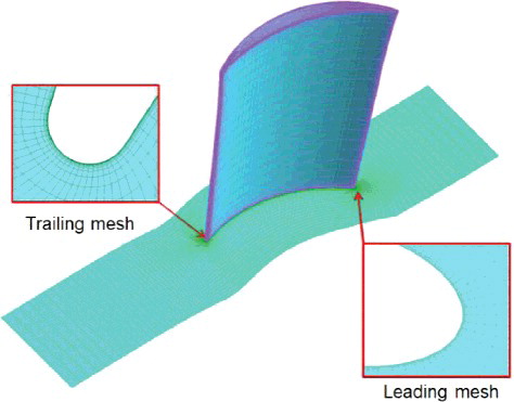
Three-dimensional numerical simulation is performed using the commercial CFD software ANSYS CFX17. The SST turbulence model is applied to close of the Reynolds-averaged turbulent Navier–Stokes equations. The O4H mesh topology is generated by grid generation tool NUMECA AutoGrid 5. To fulfill the requirement of the turbulence model, the minimum grid spacing on the solid wall is 10⁻⁶ m. This minimum grid spacing gives y + ≤ 1 at the walls. Total grid number of a single grid passage is about 400,000. The computational grids of all the calculated profiles are the same. The calculation grids are shown in Figure 5. In order to ensure the uniformity of the inlet and outlet flow field, the inlet and outlet computational domains are extended appropriately. The inlet total temperature, total pressure, flow direction and outlet static pressure are given as calculation conditions.

Figure 5. Calculation grids.

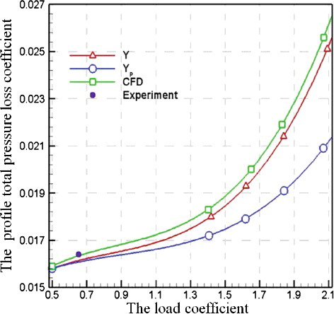
Due to the fact that the velocity triangles of the highly loaded helium compressor and the air compressor are different, the profile loss of the highly loaded helium compressor cannot be predicted by the profile loss model of air compressor accurately. As the loading coefficient increase, the exit angle will be bigger than 90°. Then the nozzle effect is becoming more and more obvious when the flow coefficient is constant. As shown in Figure 6, the deviation between the CFD value and the traditional profile loss model value is more and more obvious, but the new loss model can meet with the CFD value very well. The experimental data is obtained by Zhu [23].

Figure 6. Effect of the load coefficient on the profile loss coefficient for the compressor blade.

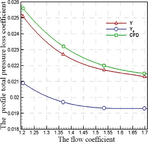
The flow coefficient is one of the important factors that affect the profile loss of highly loaded helium compressor. The inlet and outlet angles of the compressor are determined by the flow coefficient when the load coefficient and reaction are constant. Small flow coefficient lengthens the nozzle section, which will lead to the profile loss increase. As shown in Figure 7, the new profile loss model can accurately predict the profile loss coefficient at different flow coefficient.

Figure 7. Effect of the flow coefficient on the profile loss coefficient for the compressor blade.

4. Recommendations for the design of a highly loaded stage

4.1. Reaction

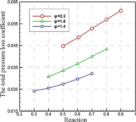
The reaction represents the percentage of pressure ratio of the rotor on that of the whole elementary stage. An appropriate reaction can effectively organize the distribution of pressure of elementary cascade and control the profile and secondary loss. Figures 8–10 illustrate the total pressure loss variation with the change of reaction when flow coefficient remains unchanged. As shown in Figures 8 and 9, the mean relative velocity of rotor blade can be lowered by a higher reaction for a given load. Because the total pressure loss is basically proportional to the square of the velocity, the loss of highly loaded helium compressor rotor blade can be reduced effectively by high reaction design, yet the stator loss will increase at the same time. Therefore, an appropriate reaction can decline the stage loss to the lowest value. Total pressure loss increases with the increase in load, when the reaction is unchanged.

Figure 8. Effect of stage load and reaction on rotor loss coefficient.

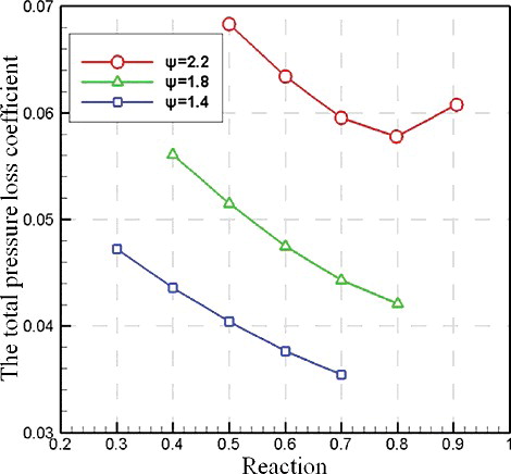
Figure 9. Effect of stage load and reaction on stator loss coefficient.

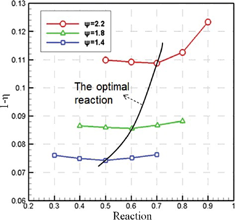
The effect of the stage loading and reaction on the total stage performance is illustrated using the lost efficiency curves (1 − η) shown in Figure 10. These curves are not a simple addition of the losses shown in Figures 8 and 9, but a composite of both the loss and velocity triangle effects.

Figure 10. Effect of stage load and reaction on stage loss.

4.2. Flow coefficient

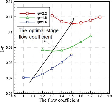
The flow coefficient has a direct influence on the compressor blade angle when the loading coefficient and the reaction are constant. The increase of the flow coefficient can effectively control the compressor blade angle and reduce the total pressure loss coefficient in the design of the high load helium compressor which can be seen from Figures 11 and 12. But the increase of the flow coefficient will increase the speed of the working fluid, thus increasing the loss. So the compressor's loss can be reduced to the minimum by a proper flow coefficient. The optimal flow coefficient of different load is shown in Figure 13.

Figure 11. Effect of stage load and flow coefficient on rotor loss coefficient.

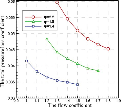
Figure 12. Effect of stage load and flow coefficient on stator loss coefficient.

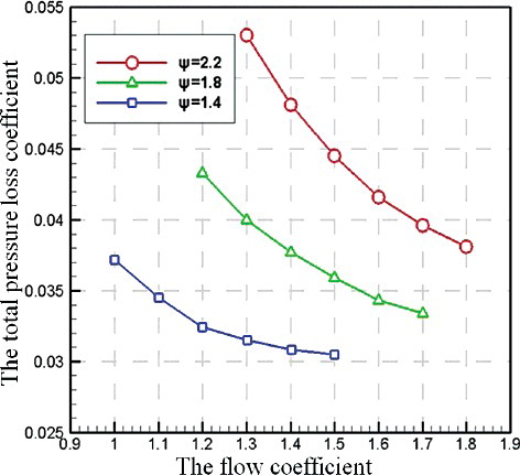
Figure 13. Effect of stage load and flow coefficient on stage loss.

4.3. Smith chart

The velocity triangle of the highly loaded helium compressor is different from that of air compressor, which is due to the differences of physical properties between helium and air. Therefore, the Smith chart of general air compressor could not be applied to the highly loaded helium compressor. In this section, the special Smith chart that is applicable to highly loaded helium compressor is drawn and analyzed based on the losses models of the previous section.

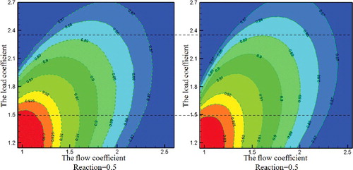
Figures 14 and 15 are the Smith charts for highly loaded helium compressor and air compressor at 0.5 reactions. The design parameter selections of the highly loaded helium compressor are different from that of the air compressor. The air compressors have high design efficiency when loading coefficient and flow coefficient are at about 0.5. But the highly loaded helium compressors have a relatively high efficiency in a wide range of flow coefficient and loading coefficient. So, large flow coefficient is beneficial for the highly loaded helium compressor design in case of high load. When designing the highly loaded helium compressor, making the flow coefficient, loading coefficient and the reaction well matched can fully play the capacity of the cascade and achieve high design efficiency.

Figure 14. Smith chart for highly loaded helium compressor at 0.5 reactions.

Figure 15. Smith chart for air compressor at 0.5 reactions [24].

There are two Smith charts which are obtained at different reactions for highly loaded helium compressor. As shown in Figure 16, the selection of the reaction can be referred to air compressor when the loading coefficient is relatively small. As the loading coefficient increasing, the optimal reaction also increases. For the design of highly loaded helium compressor, high reaction can be used to improve the efficiency. The reason is that the tolerance of rotor to adverse pressure gradient is better than that of the stator which is also found in air compressor by Tony Dickens Ivor Day [25].

Figure 16. Smith chart for different reactions.

5. Verification of the highly loaded aerodynamic design idea

5.1. Design of the highly loaded helium compressor

Based on the project of Japanese 300-MW low-pressure helium compressor [26] as a baseline design, the present highly loaded helium compressor is designed and compared with the baseline design. As shown in Table 1, the stage number is reduced from 16 to 3 to shorten the rotor; the flow coefficient and load coefficient are increased, but the aspect ratio is decreased in the highly loaded design.

Table 1. The comparison of main parameters.

Parameters	Prototype design	Highly loaded design
Inlet pressure (Mpa)	2.442	2.442
Inlet temperature (°C)	35	35
Single stage pressure ratio (1st)	1.03	1.17
Mass flow (kg/s)	178.2	178.2
Exit pressure (M pa)	3.84	3,84
Aerodynamic design pitch line values
Number of stages	16	3
Tip diameter (first rotor) (m)	1.426	1.348
Hub diameter (first stator) (m)	1.282	1.282
Tip speed (first stage) (m/s)	268.78	247.857
Rotor/stator vane/blade count (first stage)	142/167	360/394
Rotor/stator chord (first stage) (mm)	41.936/35.586	20.578/16.717
Rotor/stator solidity (first stage)	1.4/1.4	1.8/1.6
Rotor/stator aspect ratio (first stage)	1.7/2.0	1.6/1.8
Rotor tip/stator hub clearance	1% blade span	1% blade span
Flow coefficient	0.6	1.4
Load coefficient	0.32	1.8
reaction	0.7	0.7

The baseline design of the helium compressor has been considered and designed very well, but the inlet relative Mach number of the helium cascade is 0.3, which is under the maximum efficiency of airfoil. As shown in Figure 14, the stage loading and reaction must be increased together to maintain optimum efficiency for a nominal stage in a low speed compressor. The choices of stage load and stage reaction are inextricably linked. As shown in Figure 10, the proper reaction is about 0.6 with the 1.4 flow coefficient and 1.8 loading coefficient. Otherwise the baseline design also has a high degree of reaction, so the value in highly loaded design is selected as 0.7 maybe some higher value.

In order to reduce the helium compressor stages, giving fully using to the characteristics of low Mach number, the inlet axial velocity can be increased properly, so as to increase the flow coefficient, and also the single-stage pressure ratio. The relation of stage efficiency and flow coefficient is different between air and helium, shown in Figure 14. We choose the flow coefficient as 1.4 and load coefficient as 1.8 in the highly loaded design, which efficiency is just a little lower than the maximum value as shown in Figure 14.

5.2. Numerical simulation of the compressor

All the simulations were performed under steady conditions using only one periodic blade passage for the three-stage compressor in the present work. The geometric configuration of the compressor is displayed in Figure 17. The number of inlet guide vanes is 145. The number of rotors blades is 145,165,185. The number of stators blades is 155,175,195. The number of outlet guide vanes is 205. The total number of the grids is 2.8 million. The rotor tip-clearance regions are set at identical values of 1% blade span and considered with eight grid elements in spanwise direction. A high-quality H-type grid is used for both inlet and outlet blocks, while a 10-layer O-type grid is utilized for the blade's leading and trailing edges to achieve a good flow field representation.

Figure 17. Computational geometric model and grids.

In order to simulate the complicated turbulent flows correctly in this multistage compressor, a well-suited turbulence model should be selected carefully. In this study, the SST turbulence model is used for the closure of the discretized Navier–Stokes equations which is fit for highly loaded compressor and boundary layer calculation.

The total pressure and the total temperature prescribed at the three-stage highly loaded axial helium compressor inlet boundary are 2,442,000 Pa and 308 K, respectively. The circumferential average static pressure is assumed at the compressor outlet boundary (the value is 3,413,410 Pa for the compressor design operating point when mass flow rate is 178.2 kg/s). No slip and adiabatic conditions are specified on the hub, shroud and blade surfaces. The mixing approximation method is used to exchange the data of interfaces between two adjacent domains in fast steady simulation.

5.3. Result and discussions

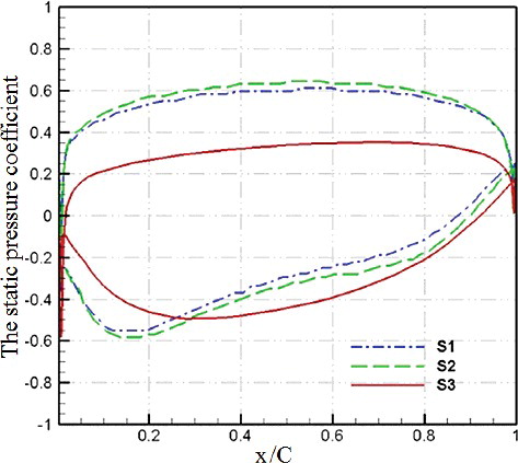
The surface static pressure distributions of highly loaded helium compressor are shown in Figures 18 and 19. From the static pressure distribution at 50% height of rotor, it can be seen that the load has increased at all chord regions. And the static pressure coefficient sustained increases from the lead edge to the trailing edge at suction surface. The negative pressure gradient is relatively big in the suction surface and small in the pressure surface. So the suction surfaces of the highly loaded helium compressor are easy to form a thick boundary layer. The distributions of the load along the span are relatively uniform for the stators. There is a large negative pressure gradient at the trailing edge of the suction surface.

Figure 18. Surface pressure coefficient distribution of rotors.

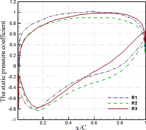
Figure 19. Surface pressure coefficient distribution of stators.

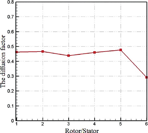
The diffusion factor of compressor plays a key role on efficiency and stability. In order to make the highly loaded helium compressor the best performer, the diffusion factors of the compressor are chosen at 0.45, which can be seen in Figure 20.

Figure 20. Diffusion factor of rotor and stator.

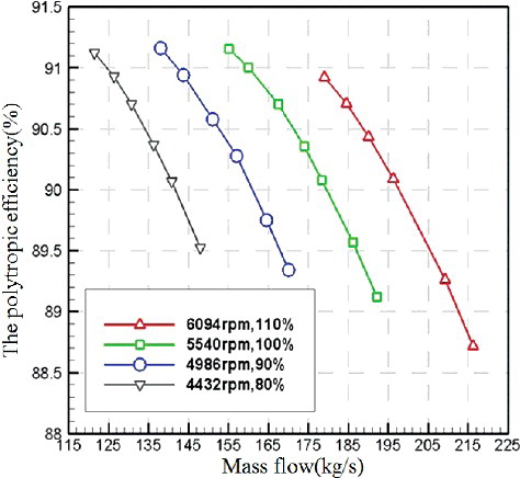
Figures 21 and 22 are the performance maps for the three-stage highly loaded axial helium compressor. Because the highly loaded velocity triangle is used, the performance maps of the highly loaded helium compressor is different with the prototype one. The pressure ratio did not increase with the decrease of the flow but decrease, the phenomenon is not prototype in the design of air compressor.

Figure 21. Speed line at the design speed for pressure ratio.

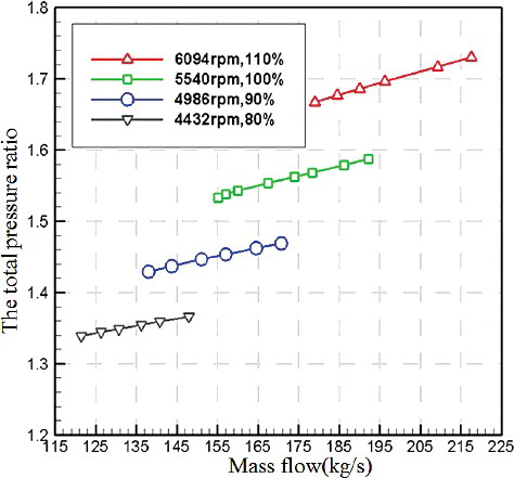
Figure 22. Speed line at the design speed for efficiency.

In compressor off-design calculation, because of the change of the outlet flow angle of rotor and the inlet flow angle of stator is small, assuming that it does not change, as shown in Figure 3. The off-design velocity triangles between highly loaded helium compressor and prototype are quite different. When the outlet pressure increases, the flow is reduced, torsion speed ∆W_u does not increase as the prototype but reduce in the premise of the circumferential velocity unchanged, namely the amount of work reduces, the helium pressure ratio decreases, and that means high load helium compressor suction surface pressure gradient does not increase by the increasing of outlet pressure and the stability of the compressor doesn't become bad .This is the key that the helium compressor can be designed based on the high load velocity triangle.

6. Conclusions

The helium compressor cascade total pressure loss model is derived by considering the thermodynamic properties differences between the helium and air and the highly loaded design characteristics. Highly loaded design methods of helium compressor are studied. The three-stage highly loaded helium compressor is designed and then CFD simulation is carried out to validate those helium highly loaded loss models and design principles proposed. Then the effect of the stage loading, the reaction and the flow coefficient on the efficiency for the highly loaded helium compressor is discussed by using the loss models. Conclusions are as follows:

(1)	The loss deviation of the air compressor and the helium compressor obtained by the traditional loss model is small at low load. So the design methods, performance maps and empirical correlations of conventional air compressor can be used as reference for helium compressor designing at low loading. With the increasing of loading, the loss deviation of the air compressor and the highly loaded helium compressor obtained by the traditional loss model becomes bigger and bigger. The blade profile loss of the highly loaded helium compressor cannot be predicted by the traditional loss models accurately. The reason is that difference of working fluid viscosity and the difference of velocity triangle result in the difference of cascade wall shear stress.
(2)	The highly loaded helium compressor loss model is obtained by considering the thermodynamic properties differences between the helium and air and the different of velocity triangle. Through the corrections, the deviation between the CFD value and the new profile loss model value can be less than 3%, which can meet with the one dimensional design very well.
(3)	By using new velocity triangle, the specific power and adverse pressure gradient of highly loaded helium compressor are decreased when backpressure is increased, which means that the highly loaded helium compressor has good aerodynamic stability.
(4)	The numerical simulation validations show that the proposed highly loaded helium compressor design method can increase the pressure ratio of the single stage helium compressor, and highly loaded helium compressor can have a comparative single stage pressure ratio as that of air compressor.

Nomenclature
Y	=	Pressure loss coefficient of a blade cascade
C	=	Actual chord length of blade (m)
H	=	Height of blades (m)
W	=	Gas relative velocity vector with respect to rotor wheel(m/s)
V	=	Gas absolute velocity vector (m/s)
U	=	Rotor tangential velocity (m/s)
D*	=	Equivalent diffusion ratio
R	=	Rotor
μ	=	Viscosity (kg*s/m2)
ρ	=	Density (kg/m3)
α	=	Angle between ∼V and meridional plane
β	=	Blade angle relative to the direction of rotation
θ	=	Equivalent expansion angle
Ф	=	Angle between ∼W and meridional plane
k	=	Isentropic index
F	=	Area
S	=	Stator
CL	=	Lift coefficient
ϕ	=	Flow coefficient
π	=	Pressure ratio
t	=	Blade thickness (m)
d	=	Pitch
ζ	=	Correction factor
ξ	=	Correction factor
ς	=	Local loss coefficient
σ	=	Blade cascade solidity (C/d)
θ2	=	Boundary-layer momentum thickness (m)
VX	=	Meridional velocity component (m/s)
CFD	=	Computational fluid dynamics
HTGR	=	High temperature gas-cooled reactor
r	=	Radius

Subscripts
p	=	Profile losses
ad	=	Additional loss
Ma	=	Maher number correction factor
l	=	Load of compressor
1	=	Inlet or leading edge
m	=	The factor of thickness
L	=	Leading edge
pr	=	Helium profile losses
A,B	=	Refrigerant
Re	=	Reynolds number
n	=	Nature of helium
2	=	Exit or trailing edge
T	=	Trailing edge

Data processing formula
Total pressure ratio	=	${\pi }^{*}=\frac{P_3^{*}}{P_1^{*}}$
Total temperature ratio	=	${\theta }^{*}=\frac{T_3^{*}}{T_1^{*}}$
Total pressure loss coefficient	=	$Y=\frac{P_1^{*}-P^{*}}{P_1^{*}-P_1}$
Pressure ratio	=	$\pi =\frac{P_3}{P_1}$
Surface pressure coefficient	=	$C_p=\frac{P-P_1}{P_1^{*}-P_1}$
Isentropic compression efficiency	=	$\eta =\frac{{\pi }^{*\frac{k-1}{k}}-1}{{\theta }^{*}-1}$

Acknowledgement

The authors wish to thank the financial supports of National Natural Science Foundation of China [Grant Number 51476039].

Disclosure statement

No potential conflict of interest was reported by the authors.

Additional information

Funding

The authors wish to thank the financial supports of National Natural Science Foundation of China [Grant Number 51476039].

References

- Yang G, Xu Y, Zheng G, et al. Characteristic analysis of rotor dynamics and experiments of active magnetic bearing for HTR-10GT. Nucl Eng Des. 2007;237:1363–1371.
- Zhang Z, Yu S. Future HTGR developments in China after the criticality of the HTR-10. Nucl Eng Des. 2002;218:249–257.
- Muto Y,Miyamoto Y, Shiozawa S. Present Activity of the Feasibility Study of HTGR-GT System. IAEA Technical Committee Meeting. Beijing (China): INET; 1998.
- Malang S, Schnauder H, Tillack M. Combination of a self-cooled liquid metal breeder blanket with a gas turbine power conversion system. Fusion Eng Des. 1998;41:561–567.
- Crommelin AK. Small-scale well-proven inherently safe nuclear power conversion. J. Eng Gas Turb Power. 2004;126(2):329–333.
- Weisbrodt IA. Summary report on technical experiences from high-temperature helium turbomachinery testing in Germany. Nuclear Power Technology Section; 1995. p. 177–248.
- Yasushi M, Shintaro I, Yoshitaka F, et al. Design study of helium turbine for the 300MW HTGR-GT power plant. ASME Turbo Expo 2000; Munich (Germany); 2000.
- Yan T, Takizuka K, Kunitomi H, et al. Aerodynamic design, model test, and CFD analysis for a multistage axial helium compressor. J Turbomach. 2008;130(3):031018–031029
- Mihayiluofu AИ, Baolisuofu BB, Kalining K. Closed cycle gas turbine plant. Book of Science Publishing Company; 1964. p. 39–57.
- Yan L, Li X, Chun X, et al. Simulation for a new cascade of helium compressor with enhanced pressure ratio. 18th International Conference on Nuclear Engineering; 2010 May 17–21; Xi'an, China.
- Ting K, Qun Z. The highly loaded aerodynamic design and performance enhancement of a helium compressor. ASME Turbo Expo 2010; 2010 June 14–18; Glasgow, UK.
- Ting K, Qun Z. Design and aerodynamic analysis of a highly loaded helium compressor. ASME Turbo Expo 2011; 2011 June 6–10; British Columbia, Canada.
- Bin J, Zhong C, Hang C, et al. Similarity and cascade flow characteristics of a highly loaded helium compressor. Nucl Eng Des. 2015; 286:286–296.
- Roberts SK, Sjolander SA. Effect of the specific heat ratio on the aerodynamicperformance of turbomachinery. J Eng Gas Turb Power. 2002;127(4):773–780.
- Roberto C, Antonio S. Influence of working fluid composition on the performance of turbomachinery in semi-closed gas turbine cycles, ASME Turbo Expo 2012; 2012 June 11–15; Copenhagen, Denmark.
- Lieblein S. Loss and stall analysis in compressor cascades. J Basic Eng. 1959;81:387–400.
- Lieblein S, Johnsen I. Résumé of transonic-compressor research at NACA Lewis Laboratory. J Eng Gas Turb Power. 1961;83(3):219–232.
- Koch CC, Jr. Smith LH., Loss sources and magnitudes in axial-flow compressors. J Eng Power. 1976; 98(3): 411–424.
- Howell AR. Fluid dynamics of axial compressors. Lectures on the development of the British gas turbine jet unit, War Emergency Proceedings No. 12; Institution of Mechanical Engineers; 1947; Great Britain; p. 441–52.
- Aungier RH. A strategy for aerodynamic design and analysis. New York (NY): ASME Press; 2003. p. 118–52.
- Yaras MI, Sjolander SA. Prediction of tip-leakage losses in axial turbines. J Turbomach. 1992;114:204–10.
- Dixon SL, Hall CA. Fluid mechanics and thermodynamics of turbomachinery. Butterworth-Heinemann; 2010. Chapter 5; pp. 146–147.
- Rongkai Z. Researches of similitude theory for axial flow helium compressor. [dissertation]; 2008.
- Wright P, Miller D. An improved compressor performance prediction model. Proceedings of the European Conference of Turbomachinery: Latest Developments in a Changing Scene; 1991; Paper No. C423/028.
- Tony D. The design of highly loaded axial compressors. J Turbomach. 2011;133(3):57–67.
- Yasushi M, Shintaro I. Design study of helium turbine for the 300mw HTGR-GT power plant. ASME Turbo Expo; 2000; Munich, Germany.