Improvements and validation of the transient analysis code MOREL for molten salt reactors

ABSTRACT

The liquid fuel salt used in the molten salt reactors (MSRs) serves as the fuel and coolant simultaneously. On the one hand, the delayed neutron precursors circulate in the whole primary loop and part of them decay outside the core. On the other hand, the fission heat is carried off directly by the fuel flow. These two features require new analysis method with the coupling of fluid flow, heat transfer and neutronics. In this paper, the recent update of MOREL code is presented. The update includes: (1) the improved quasi-static method for the kinetics equation with convection term is developed. (2) The multi-channel thermal hydraulic model is developed based on the geometric feature of MSR. (3) The Variational Nodal Method is used to solve the neutron diffusion equation instead of the original analytic basis functions expansion nodal method. The update brings significant improvement on the efficiency of MOREL code. And, the capability of MOREL code is extended for the real core simulation with feedback. The numerical results and experiment data gained from molten salt reactor experiment (MSRE) are used to verify and validate the updated MOREL code. The results agree well with the experimental data, which prove the new development of MOREL code is correct and effective.

KEYWORDS:

• Molten salt reactor
• neutronics
• thermal hydraulics
• dynamics

1. Introduction

The molten salt reactor (MSR) is the only one using liquid fuel in six candidates of Generation IV reactor type [1]. The fuel like UF4 or ThF4 is dissolved in the fluoride salt [2]. The liquid fuel salt circulates through the primary loop and acts as both the fuel and the coolant simultaneously [3].

In the neutronics aspect, the delayed neutron precursors (DNPs) in the MSR continuously change their position and part of them may decay outside the core and the others will re-enter the reactor core. It leads to the reactivity loss and effective delayed neutron fraction decrease [4]. In the thermal-hydraulics (TH) aspect, the liquid fuel also acts as the heating medium, which carries off the heat produced by fission reactions. Meanwhile, the graphite in the core also produces heat due to the fuel permeation and gamma irradiation and it is cooled by the liquid fuel [5]. Therefore, the fuel salt circulation brings strong coupling between neutronics and TH calculation. Those features bring significant differences for the MSR from the conventional reactors using the solid fuel.

Many efforts focusing on the transient behavior and safety performance of different MSRs have been carried out by different researchers. And, many methods and codes have been developed. Kophazi et al. adopted a modified version of MCNP4C code to model the liquid fuel [6]. Wang et al. focused on the simulation of TH behavior and optimized the MOSART design using the SIMMER-III code [7,8]. Krepel et al. developed the DYN1D-MSR and DYN3D-MSR codes for the safety analysis on the graphite-moderated channel-type MSR [9,10]. Lecarpentier and Carpentier developed the Cinsf1D code for the one-dimensional calculation based on the two-group diffusion theory [11]. Guo et al. developed the safety analysis code based on the point reactor kinetic model [12]. Dulla developed the POLITO code by adopting the quasi-static approximation in the two-dimensional (2D) cylindrical geometry [13]. Zhang et al. studied the MOSART reactor based on the control volume method for the two-group 3D diffusion solution [14,15]. It should be noted that various hypotheses and some deficiencies exist. MCNP4C is not capable of transient simulation; Quasi-static (QS) approximation employed in POLITO has a low accuracy; Zhang et al. and DYN1D/3D-MSR take much computational time due to Backward Euler method for time-discretization; Cinsf1D and Guo et al. employ 1D and point reactor kinetic model to simulate MSR neutronics, respectively.

In our previous paper, a comprehensive and special code named MOREL was developed for the MSR kinetics analysis [16]. However, some shortages of MOREL were encountered in the practical analysis of an MSR core. First, coupling between the neutronics and TH calculation is not considered. Second, the flux reconstruction used for DNP source calculation takes extra computational cost and difficulties. Third, the efficiency is too low in practical core analysis because of using the Analytic Basis Functions Expansion Nodal (ABFEN) method for spatial discretization and the Backward Euler method for time discretization.

To overcome those deficiencies of previous research and MOREL code, some new kernels and methods are introduced and a new updated code named MOREL2.0 is developed to provide a deeper insight into the characteristics of MSR. By comparison with previous research, 3D time-space neutron dynamics model based on Predictor-Corrector Improved Quasi-Static method (PCIQS) is adopted in this paper for better efficiency and accuracy. By comparison with MOREL, first, the PCIQS method for the liquid fuel reactor is employed to improve the efficiency in the kinetics calculations. Second, the multi-channel TH model is employed based on the geometric feature of MSR and coupling between neutronics and TH is realized in MOREL2.0 to consider realistic TH feedback. Third, Variational Nodal Method (VNM) is employed, which is more efficient than ABFEN method employed in MOREL in solving 3D diffusion equation due to the following advantages: (1) the fine flux distribution can be obtained easily without the flux reconstruction and (2) accuracy and convergency can be guaranteed theoretically [17].

Numerical verification and validation are done based on the comparisons with different codes and against the experimental data from MSRE [5]. The models and new kernels in the updated code MOREL2.0 are described in Section 2. The numerical results are presented in Section 3. Finally, some conclusions are summarized to close the paper inSection 4.

2. Mathematic model and numerical method

The updated MOREL code is named MOREL2.0 in this paper. Several new models have been put into the new code and will be discussed in the following sections.

2.1. Homogenized few group parameters

In the MOREL2.0 code, the 2D lattice code HELIOS based on the ENDF/B-VI library is inherited to generate the homogenized few-group cross-sections for different fuel temperature (TF) and graphite temperature (TG) [18]. The relationship as in Equation (1)(1) $$\begin{array}{c}\hfill {\rho }_{\mathrm{salt}}=2.263\times (1-2.12\times {10}^{-4}\times (T\left(K\right)-923))\end{array}$$(1) between the fuel density and fuel temperature is used in the case matrix while calculating the cross sections. The least square fitting method is adopted to generate the cross section table, which is optimized for better consideration of feedback effect. (1) $$\begin{array}{c}\hfill {\rho }_{\mathrm{salt}}=2.263\times (1-2.12\times {10}^{-4}\times (T\left(K\right)-923))\end{array}$$(1) where the unit of ρ is g/cm³.

2.2. 3D time-dependent neutron diffusion equation for MSR

The multi-group time-space depended neutron kinetics equations are given in Equations (2) and (3(3) $$\begin{array}{ccc}\hfill \frac{\partial C_i(r,t)}{\partial t}& =& {\beta }_i{S}_F(r,t)-{\lambda }_i{C}_i(r,t)\hfill \\ & & -\nabla \left[U(r,t)C_i(r,t)\right],i=1,2,...,I\hfill \end{array}$$(3) ), respectively. (2) $$\begin{array}{ccc}\hfill \frac{1}{v_g}\frac{\partial {\varphi }_g(r,t)}{\partial t}& =& \nabla ·D_g(r,t)\nabla {\varphi }_g(r,t)-{\Sigma }_{tg}(r,t){\varphi }_g(r,t)\hfill \\ & & +\sum _{g^{\text{'}}=1}^G{\Sigma }_{g\text{'}g}(r,t){\varphi }_{g^{\text{'}}}(r,t)+(1-\beta )\hfill \\ & & \times {\chi }_{pg}{S}_F(r,t)+\sum _{i=1}^I{\chi }_{dgi}{\lambda }_i{C}_i(r,t)\hfill \\ \hfill g& =& 1,2,...,G,i=1,2,...I\hfill \end{array}$$(2) (3) $$\begin{array}{ccc}\hfill \frac{\partial C_i(r,t)}{\partial t}& =& {\beta }_i{S}_F(r,t)-{\lambda }_i{C}_i(r,t)\hfill \\ & & -\nabla \left[U(r,t)C_i(r,t)\right],i=1,2,...,I\hfill \end{array}$$(3) where ϕ is the scalar flux. C is the DNP density. U is the vector of fuel velocity. G and I are the total number of group and delayed neutron families, respectively. Standard notations are used for the macroscopic cross sections. S_F is the total fission source defined as: (4) $$\begin{array}{c}\hfill S_F(r,t)=\frac{1}{k_{\mathrm{eff}}^s}\sum _{g^{\text{'}}=1}^G\nu {\Sigma }_{f{g}^{\text{'}}}(r,t){\varphi }_{g^{\text{'}}}(r,t)\end{array}$$(4) where k^s_eff is an effective multiplication factor at steady state.

The flow of liquid fuel brings little effect on the prompt flux but large effect on the DNP distribution. As a result, an additional convective term is introduced into the balance equation of DNP.

There are several methods used for solving the time-dependent neutron diffusion equation, include the theta method, backward differentiation formula (BDF) method [19] and so on. A detailed discussion of these methods can be found in [20]. Among these methods, the Backward Euler method is the most popular one for its numerical stability. For a given time step interval Δt_n=t_n − t_n-1 at the nth time step, the left-hand side of Equation (2)(2) $$\begin{array}{ccc}\hfill \frac{1}{v_g}\frac{\partial {\varphi }_g(r,t)}{\partial t}& =& \nabla ·D_g(r,t)\nabla {\varphi }_g(r,t)-{\Sigma }_{tg}(r,t){\varphi }_g(r,t)\hfill \\ & & +\sum _{g^{\text{'}}=1}^G{\Sigma }_{g\text{'}g}(r,t){\varphi }_{g^{\text{'}}}(r,t)+(1-\beta )\hfill \\ & & \times {\chi }_{pg}{S}_F(r,t)+\sum _{i=1}^I{\chi }_{dgi}{\lambda }_i{C}_i(r,t)\hfill \\ \hfill g& =& 1,2,...,G,i=1,2,...I\hfill \end{array}$$(2) or (3(3) $$\begin{array}{ccc}\hfill \frac{\partial C_i(r,t)}{\partial t}& =& {\beta }_i{S}_F(r,t)-{\lambda }_i{C}_i(r,t)\hfill \\ & & -\nabla \left[U(r,t)C_i(r,t)\right],i=1,2,...,I\hfill \end{array}$$(3) ) can be discretized using the Backward Euler method as: (5) $$\begin{array}{c}\hfill \frac{A^n\left(r\right)-A^{n-1}\left(r\right)}{B^n}=R^n\left(r\right)\end{array}$$(5) where A is flux or DNP density, Rⁿ denotes all the right-hand side term of Equation (2)(2) $$\begin{array}{ccc}\hfill \frac{1}{v_g}\frac{\partial {\varphi }_g(r,t)}{\partial t}& =& \nabla ·D_g(r,t)\nabla {\varphi }_g(r,t)-{\Sigma }_{tg}(r,t){\varphi }_g(r,t)\hfill \\ & & +\sum _{g^{\text{'}}=1}^G{\Sigma }_{g\text{'}g}(r,t){\varphi }_{g^{\text{'}}}(r,t)+(1-\beta )\hfill \\ & & \times {\chi }_{pg}{S}_F(r,t)+\sum _{i=1}^I{\chi }_{dgi}{\lambda }_i{C}_i(r,t)\hfill \\ \hfill g& =& 1,2,...,G,i=1,2,...I\hfill \end{array}$$(2) or (3(3) $$\begin{array}{ccc}\hfill \frac{\partial C_i(r,t)}{\partial t}& =& {\beta }_i{S}_F(r,t)-{\lambda }_i{C}_i(r,t)\hfill \\ & & -\nabla \left[U(r,t)C_i(r,t)\right],i=1,2,...,I\hfill \end{array}$$(3) ) at the time step n, and Bis defined as v_gΔt_n or Δt_n.

In the previous MOREL code, the Backward Euler method was adopted. It gave good results, but the computational efficiency was not satisfying for the limitation of fine time step requirement. It is improved by using the new quasi-static method for MSR as described in Section 2.4.

2.3. Variational nodal method

Different from the original MOREL, the VNM method is applied as the kernel of solving the neutron diffusion equation. The new kernel is more computationally efficient and it will be discussed in Section 3.1.

Source iteration method is employed in VNM to solve diffusion equation, and source iteration includes two iteration steps: scattering source iteration and fission source iteration. In the MSR neutronics calculation, the diffusion equation and DNP equation sets need to be solved separately and coupled with each other by the source term during fission source iteration even for the eigenvalue calculation at steady state, where Δt_{n + 1} comes close to infinity in Equation (5)(5) $$\begin{array}{c}\hfill \frac{A^n\left(r\right)-A^{n-1}\left(r\right)}{B^n}=R^n\left(r\right)\end{array}$$(5) .

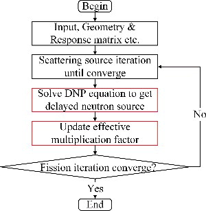
Figure 1 presents the calculation flowchart of the eigenvalue calculation for MSR and there are some differences in comparison with traditional solid fuel reactor. The scattering source iteration is followed by solving DNP equation, then effective multiplication factor is updated by Equation (6)(6) $$\begin{array}{c}\hfill k_{eff}^s=\frac{{\int }_r{\sum }_{g=1}^G\left(1-\beta \right){\chi }_{pg}{\sum }_{g^{\text{'}}=1}^G\nu {\Sigma }_{f{g}^{\text{'}}}\left(r\right){\phi }_{g^{\text{'}}}^n\left(r\right)dr+{\int }_r{\sum }_{g=1}^G\left({\sum }_{i=1}^I{\chi }_{dgi}{\lambda }_i{C}_i^n\left(r,t\right)\right)dr}{\frac{1}{k_{eff}^{s,n-1}}\left({\int }_r{\sum }_{g=1}^G\left(1-\beta \right){\chi }_{pg}{\sum }_{g^{\text{'}}=1}^G\nu {\Sigma }_{f{g}^{\text{'}}}\left(r\right){\phi }_{g^{\text{'}}}^{n-1}\left(r\right)dr+{\int }_r{\sum }_{g=1}^G\left({\sum }_{i=1}^I{\chi }_{dgi}{\lambda }_i{C}_i^{n-1}\left(r,t\right)\right)dr\right)}\end{array}$$(6) . This process always repeat until the fission source and eigenvalue converge as described in Figure 1. Accordingly, the fission source for MSR in steady state is required to be divided into two parts: the prompt neutron source and the delayed neutron source. (6) $$\begin{array}{c}\hfill k_{eff}^s=\frac{{\int }_r{\sum }_{g=1}^G\left(1-\beta \right){\chi }_{pg}{\sum }_{g^{\text{'}}=1}^G\nu {\Sigma }_{f{g}^{\text{'}}}\left(r\right){\phi }_{g^{\text{'}}}^n\left(r\right)dr+{\int }_r{\sum }_{g=1}^G\left({\sum }_{i=1}^I{\chi }_{dgi}{\lambda }_i{C}_i^n\left(r,t\right)\right)dr}{\frac{1}{k_{eff}^{s,n-1}}\left({\int }_r{\sum }_{g=1}^G\left(1-\beta \right){\chi }_{pg}{\sum }_{g^{\text{'}}=1}^G\nu {\Sigma }_{f{g}^{\text{'}}}\left(r\right){\phi }_{g^{\text{'}}}^{n-1}\left(r\right)dr+{\int }_r{\sum }_{g=1}^G\left({\sum }_{i=1}^I{\chi }_{dgi}{\lambda }_i{C}_i^{n-1}\left(r,t\right)\right)dr\right)}\end{array}$$(6) where n is the number of fission iteration.

Figure 1. Flow scheme for eigenvalue calculation.

2.4. Predictor-corrector quasi-static method

The Predictor-Corrector Improved Quasi-Static (PCIQS) method for neutronics kinetics equation with convection term is adopted in the MOREL2.0 code. The PCIQS method allows a reduction of computational time significantly in the transient simulations [21]. However, particular treatments need to be done for the reactor using liquid fuel. This is due to the spatial effects DNP re-distribution from fuel flow.

Referring to the works by Akcasu, it makes sense physically to use a proper mathematically adjoint solution to Equation (2)(2) $$\begin{array}{ccc}\hfill \frac{1}{v_g}\frac{\partial {\varphi }_g(r,t)}{\partial t}& =& \nabla ·D_g(r,t)\nabla {\varphi }_g(r,t)-{\Sigma }_{tg}(r,t){\varphi }_g(r,t)\hfill \\ & & +\sum _{g^{\text{'}}=1}^G{\Sigma }_{g\text{'}g}(r,t){\varphi }_{g^{\text{'}}}(r,t)+(1-\beta )\hfill \\ & & \times {\chi }_{pg}{S}_F(r,t)+\sum _{i=1}^I{\chi }_{dgi}{\lambda }_i{C}_i(r,t)\hfill \\ \hfill g& =& 1,2,...,G,i=1,2,...I\hfill \end{array}$$(2) as the weighting vector [22]. The adjoint equation of MSRs can be defined as [23]: (7) $$\begin{array}{ccc}\hfill \left({\widehat{L}}^{*}+{\widehat{M}}_p^{*}\right){\varphi }^{*}\left(r\right)+\sum _{i=1}^I{\widehat{F}}_{di}^{*}{C}_i^{*}\left(r\right)& =& 0\hfill \\ \hfill {\widehat{M}}_{di}^{*}{\varphi }^{*}\left(r\right)-\left({\lambda }_i+u\left(r\right)\frac{\partial }{\partial z}\right)C_i^{*}\left(r\right)& =& 0\hfill \end{array}$$(7) where ϕ*, C*_i is adjoint flux and adjoint DNP density, respectively; i is identifier of DNPs families; u is axial velocity of fuel salt; standard notations are used for the macroscopic cross sections and operators are described as: (8) $$\begin{array}{ccc}\hfill {\widehat{L}}^{*}& =& \nabla ·D_g\left(r\right)\nabla -{\Sigma }_t\left(r\right)·\hfill \\ \hfill {\widehat{M}}_p^{*}& =& \sum _{g^{\text{'}}=1}^G{\Sigma }_{g{g}^{\text{'}}}\left(r\right)·+(1-\beta )\frac{1}{k_{eff}}\sum _{g^{\text{'}}=1}^G{\chi }_{p{g}^{\text{'}}}\nu {\Sigma }_{fg}\left(r\right)·\hfill \\ \hfill {\widehat{F}}_{di}^{*}& =& \frac{1}{k_{eff}}{\beta }_i\nu {\Sigma }_{fg}\left(r\right)·{\widehat{M}}_{di}^{*}={\lambda }_i\sum _{g=1}^G{\chi }_{dgi}·\hfill \end{array}$$(8)

All the fuel salt flows along axial direction in the channel constructed by graphite for MSRE-type MSR, which is analyzed in this paper. Radial flow of DNP is neglected and 1D DNP model is applied in adjoint Equation (7)(7) $$\begin{array}{ccc}\hfill \left({\widehat{L}}^{*}+{\widehat{M}}_p^{*}\right){\varphi }^{*}\left(r\right)+\sum _{i=1}^I{\widehat{F}}_{di}^{*}{C}_i^{*}\left(r\right)& =& 0\hfill \\ \hfill {\widehat{M}}_{di}^{*}{\varphi }^{*}\left(r\right)-\left({\lambda }_i+u\left(r\right)\frac{\partial }{\partial z}\right)C_i^{*}\left(r\right)& =& 0\hfill \end{array}$$(7) .

The Point Kinetics Equations (PKEs) can be derived by integrating the time-dependent diffusion equation defined in Equations (2) and (3(3) $$\begin{array}{ccc}\hfill \frac{\partial C_i(r,t)}{\partial t}& =& {\beta }_i{S}_F(r,t)-{\lambda }_i{C}_i(r,t)\hfill \\ & & -\nabla \left[U(r,t)C_i(r,t)\right],i=1,2,...,I\hfill \end{array}$$(3) ) using the adjoint flux as the weight function [24]. The PKE equations for MSRs can be written as: (9) $$\begin{array}{ccc}\hfill {\displaystyle \frac{dn\left(t\right)}{dt}}& =& {\displaystyle \frac{\rho \left(t\right)-\bar{\beta }\left(t\right)}{\Lambda \left(t\right)}n\left(t\right)+\sum _i{\lambda }_i{T}_i\left(t\right)}\hfill \\ \hfill {\displaystyle \frac{d{T}_i\left(t\right)}{dt}}& =& {\displaystyle \frac{\bar{\beta }\left(t\right)}{\Lambda \left(t\right)}n\left(t\right)-{\xi }_i{T}_i\left(t\right)}\hfill \end{array}$$(9)

where n represents the neutron amplitude function, T_i and ξ_i are the amplitude function and general decay constant for the ith DNP family, respectively. The reactivity, delayed neutron fractions, neutron generation time, and delayed neutron constants are defined as: (10) $$\begin{array}{c}\hfill \\ \hfill F\left(t\right)=⟨{\varphi }_g^{*}\left(r\right),{\chi }_{pg}{S}_F\left(r,t\right)⟩\end{array}$$(10) (11) $$\begin{array}{c}\hfill {\bar{\beta }}_i=\frac{⟨{\varphi }_g^{*}\left(r\right),{\beta }_i\left(r\right){\chi }_{pg}{S}_F\left(r,t\right)⟩}{F\left(t\right)}\end{array}$$(11) (12) $$\begin{array}{c}\hfill \bar{\beta }=\sum _{i=1}^I{\beta }_i\end{array}$$(12) (13) $$\begin{array}{ccc}& & \rho \left(t\right)=\frac{1}{F\left(t\right)}\hfill \\ & & \left\{\begin{array}{c}⟨{\varphi }_g^{*}\left(r\right),{\psi }_g(r,t)\left({\Sigma }_{tg}(r,t_0)-{\Sigma }_{tg}(r,t)\right)⟩\hfill \\ +⟨{\varphi }_g^{*}\left(r\right),\sum _{g^{\text{'}}=1}^G\left({\Sigma }_{g^{\text{'}}-g}(r,t)-{\Sigma }_{g^{\text{'}}-g}(r,t_0\right){\psi }_{g^{\text{'}}}(r,t)⟩\hfill \\ +⟨{\varphi }_g^{*}\left(r\right),\sum _{g^{\text{'}}=1}^G\left[{\chi }_{pg}\left(t\right)\nu {\Sigma }_{f{g}^{\text{'}}}(r,t)-{\chi }_{pg}\left(t_0\right){\Sigma }_{f{g}^{\text{'}}}(r,t_0)\right]{\psi }_{g^{\text{'}}}(r,t)⟩\hfill \\ +⟨{\psi }_g\left(r,t\right),\nu {\Sigma }_{fg}\left(r,t_0\right)\left[\sum _{i=1}^I{\beta }_i\left(\sum _{g^{\text{'}}=1}^G{\chi }_{p{g}^{\text{'}}}{\varphi }_{g^{\text{'}}}^{*}\left(r\right)-C_i^{*}\right)\right]⟩\hfill \end{array}\right\}\hfill \end{array}$$(13) (14) $$\begin{array}{c}\hfill \Lambda \left(t\right)=\frac{1}{F\left(t\right)}⟨{\varphi }_g^{*}\left(r\right),\frac{1}{v_g}{\psi }_g(r,t)⟩\end{array}$$(14) (15) $$\begin{array}{c}\hfill {\xi }_i\left(t\right)={\lambda }_i+⟨{\varphi }_g^{*}\left(r\right),{\chi }_{dgi}\frac{\partial \left[u\left(r,t\right)c_i(r,t)\right]}{\partial z}⟩\end{array}$$(15) where subscript g and i represent the index of energy group and DNP family, respectively; ψ and c are the flux and DNP density shape function in PCIQS method, respectively [21]; t₀ means the initial time; u is the fuel flow velocity in axial direction; S_F refers to Equation (4)(4) $$\begin{array}{c}\hfill S_F(r,t)=\frac{1}{k_{\mathrm{eff}}^s}\sum _{g^{\text{'}}=1}^G\nu {\Sigma }_{f{g}^{\text{'}}}(r,t){\varphi }_{g^{\text{'}}}(r,t)\end{array}$$(4) ; standard notations are used for the macroscopic cross sections.

Compared with the popular form for the traditional reactor using solid fuel, some new additional terms are involved in Equations (10)(10) $$\begin{array}{c}\hfill \\ \hfill F\left(t\right)=⟨{\varphi }_g^{*}\left(r\right),{\chi }_{pg}{S}_F\left(r,t\right)⟩\end{array}$$(10) through (15(15) $$\begin{array}{c}\hfill {\xi }_i\left(t\right)={\lambda }_i+⟨{\varphi }_g^{*}\left(r\right),{\chi }_{dgi}\frac{\partial \left[u\left(r,t\right)c_i(r,t)\right]}{\partial z}⟩\end{array}$$(15) ) for the MSR using liquid fuel. The fourth inner product term in Equation (13)(13) $$\begin{array}{ccc}& & \rho \left(t\right)=\frac{1}{F\left(t\right)}\hfill \\ & & \left\{\begin{array}{c}⟨{\varphi }_g^{*}\left(r\right),{\psi }_g(r,t)\left({\Sigma }_{tg}(r,t_0)-{\Sigma }_{tg}(r,t)\right)⟩\hfill \\ +⟨{\varphi }_g^{*}\left(r\right),\sum _{g^{\text{'}}=1}^G\left({\Sigma }_{g^{\text{'}}-g}(r,t)-{\Sigma }_{g^{\text{'}}-g}(r,t_0\right){\psi }_{g^{\text{'}}}(r,t)⟩\hfill \\ +⟨{\varphi }_g^{*}\left(r\right),\sum _{g^{\text{'}}=1}^G\left[{\chi }_{pg}\left(t\right)\nu {\Sigma }_{f{g}^{\text{'}}}(r,t)-{\chi }_{pg}\left(t_0\right){\Sigma }_{f{g}^{\text{'}}}(r,t_0)\right]{\psi }_{g^{\text{'}}}(r,t)⟩\hfill \\ +⟨{\psi }_g\left(r,t\right),\nu {\Sigma }_{fg}\left(r,t_0\right)\left[\sum _{i=1}^I{\beta }_i\left(\sum _{g^{\text{'}}=1}^G{\chi }_{p{g}^{\text{'}}}{\varphi }_{g^{\text{'}}}^{*}\left(r\right)-C_i^{*}\right)\right]⟩\hfill \end{array}\right\}\hfill \end{array}$$(13) denotes the loss of reactivity caused by the re-distribution of DNP. And the general decay constant as in Equation (15)(15) $$\begin{array}{c}\hfill {\xi }_i\left(t\right)={\lambda }_i+⟨{\varphi }_g^{*}\left(r\right),{\chi }_{dgi}\frac{\partial \left[u\left(r,t\right)c_i(r,t)\right]}{\partial z}⟩\end{array}$$(15) involves two parts: the first part represents the intrinsic decay characteristic and the second part considers the decay of DNPs in the external loop and effect of DNP return to reactor core.

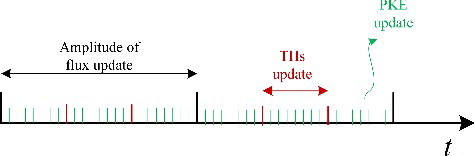
The PCIQS method factorizes the flux into the spatial shape function and the amplitude function. Different time steps can be set by its physical variation during the transients. As illustrated in Figure 2, the horizontal right arrow means time axis and the black, red and green time division represent coarse, intermediate and micro time step, respectively. One coarse time step contains several intermediate time steps and one intermediate time step covers some micro time steps. By comparison with coarse time step, the intermediate and micro time step is generally reduced by one and two orders of magnitude, respectively. The coarse time step is used to update the 3D spatial shape function in several seconds generally, since its time variation is generally slower than the changes of TH parameters and the amplitude of flux. Due to TH parameters change more slowly than neutronics parameters, the multi-channel TH solver is invoked in the intermediate time step in order to consider the feedback and update TH parameters. Finally, the time step of PKE calculation is the smallest one, which aims to capture the time variation of flux magnitude, which is driven by the prompt neutron generation time. The amplitude of flux used in the intermediate time step is calculated by interpolation based on the amplitude function at the start and endpoints of the coarse time step.

Figure 2. Illustration of PCIQS scheme.

2.5. Delayed neutron precursor drift

The MOREL2.0 code is developed for the analysis of MSRE-type MSR. The fuel salt enters the reactor core through the bottom plenum. Then, it is distributed to the individual channels and flows upward through the core. After mixed in the top collecting plenum, the fuel salt flows out of the core. So, the 1D DNP model is kept in the MOREL2.0 code, and the time derivation term in Equation (3) is discretized by BDF method at time step t_n and time step interval is defined as Δt_n=t_n − t_n-1. The discretization equation without DNP family index i is described as: (16) $$\begin{array}{c}\hfill {\displaystyle Q\left(r,t_n\right)-\zeta C(r,t_n)-\frac{\partial \left[u\left(r,t_n\right)C(r,t_n)\right]}{\partial z}=0}\end{array}$$(16) where ζis called the general decay constant of DNP and it is defined as $\zeta =\lambda +1/\phantom{1\Delta t_n}\Delta t_n$;λ is the intrinsic decay constant of DNP; Q(r, t_n) presents general DNP source that is related to both DNP source at present time step and DNP density at last time step, and it is defined as: (17) $$\begin{array}{c}\hfill Q\left(r,t_n\right)=\sum _{g^{\text{'}}=1}^G\beta \nu {\Sigma }_{f{g}^{\text{'}}}(r,t_n){\varphi }_{g^{\text{'}}}(r,t_n)+\frac{C(r,t_{n-1})}{\Delta t_n}\end{array}$$(17) where g is the specifier of energy group; G is the total number of energy of group; standard notation of neutronics is used for other symbols. And the prompt neutron flux is given by the VNM calculation in form of second order polynomials and Q(r, t_n) is expressed as: (18) $$\begin{array}{c}\hfill Q\left(r,t_n\right)=a_0\left(r,t_n\right)+a_1\left(r,t_n\right)z+a_2\left(r,t_n\right)z^2\end{array}$$(18) where a₀, a₁ and a₂ are the coefficients from the radial integration of fission source.

The neutron diffusion equation is solved only in the reactor core, but the DNP balance equation is solved for the whole primary loop. The finite difference method is employed for the solution of Equation (16)(16) $$\begin{array}{c}\hfill {\displaystyle Q\left(r,t_n\right)-\zeta C(r,t_n)-\frac{\partial \left[u\left(r,t_n\right)C(r,t_n)\right]}{\partial z}=0}\end{array}$$(16) . To guarantee the accuracy, the small mesh size of 1cm is adopted in this paper. Therefore, the axial sub-meshes are used inside the nodes for the VNM calculation.

It can be seen that the format of discretization Equation (16)(16) $$\begin{array}{c}\hfill {\displaystyle Q\left(r,t_n\right)-\zeta C(r,t_n)-\frac{\partial \left[u\left(r,t_n\right)C(r,t_n)\right]}{\partial z}=0}\end{array}$$(16) is the same with steady DNP balance equation, where the time derivation term is neglected in Equation (3)(3) $$\begin{array}{ccc}\hfill \frac{\partial C_i(r,t)}{\partial t}& =& {\beta }_i{S}_F(r,t)-{\lambda }_i{C}_i(r,t)\hfill \\ & & -\nabla \left[U(r,t)C_i(r,t)\right],i=1,2,...,I\hfill \end{array}$$(3) . Therefore, they can be solved by the same method. The external loop is also divided into a number of fine meshes along the forward direction. For the calculations in external loop, it is a pure decay problem without DNP source. The solution is easy to get in the analytical form. The DNP density in the core and external loop are obtained as:

DNP density in the core: (19) $$\begin{array}{ccc}& & C\left(x,y,z_{j+1},t_n\right)\hfill \\ & & =\left(\begin{array}{c}{\displaystyle {\int }_{z_j}^{z_{j+1}}\frac{Q\left(x,y,z^{\text{'}},t_n\right)}{u}exp\left(\frac{\zeta }{u}\left(z^{\text{'}}-z_j\right)\right)d{z}^{\text{'}}+}\hfill \\ C\left(x,y,z_j,t_n\right)\hfill \end{array}\right)\hfill \\ & & \times exp\left(-\frac{\zeta }{u}\left(z_{j+1}-z_j\right)\right)\hfill \end{array}$$(19)

DNP density in the external loop: (20) $$\begin{array}{ccc}& & C\left(x,y,z_{j+1},t_n\right)\hfill \\ & & =C\left(x,y,z_j,t_n\right)exp\left(-\frac{\zeta }{u}\left(z_{j+1}-z_j\right)\right)\hfill \end{array}$$(20) where position r is described as (x, y, z); j is the index of mesh for the one-dimensional DNP calculation. u is the axial velocity of fuel salt obtained from the TH calculation and it is assumed as constant in each mesh; other symbols has the same meaning shown in Equation (16)(16) $$\begin{array}{c}\hfill {\displaystyle Q\left(r,t_n\right)-\zeta C(r,t_n)-\frac{\partial \left[u\left(r,t_n\right)C(r,t_n)\right]}{\partial z}=0}\end{array}$$(16) .

Two boundaries are considered in the calculation of DNP distribution.

1)	The un-decayed DNPs which reenters the core is defined as: (21) $$\begin{array}{c}\hfill C_{i,in}=C_{i,out}·exp\left(-{\lambda }_i·\tau \right)\end{array}$$(21)

where C is DNP density; i is index of DNP family; in means DNP reenter the reactor core; out means DNP flow out of reactor core; τis the circulation time of fuel salt in external loop.

2)	The flow of DNP is kept constant from the core outlet to the inlet.

2.6. Thermal hydraulics

In this paper, the modeled reactors are composed of three axial regions, including the bottom and top plenum and the active core with graphite moderator. In current calculation, no fuel boiling is considered. So, in the TH model, a set of one-phase 1D equations for the liquid fuel is established.

The mass balance equation is defined as: (22) $$\begin{array}{c}\hfill \frac{\partial }{\partial t}\left(\rho \right)+\frac{\partial }{\partial z}\left(\rho v\right)=0\end{array}$$(22)

The energy balance equation is presented as: (23) $$\begin{array}{c}\hfill \frac{\partial }{\partial t}\left(\rho h\right)+\frac{\partial }{\partial z}\left(\rho vh\right)=Q^f\end{array}$$(23)

The momentum balance equation is: (24) $$\begin{array}{c}\hfill \frac{\partial }{\partial t}\left(\rho v\right)+\frac{\partial }{\partial z}\left(\rho v^2\right)+\frac{\partial P_{fric}}{\partial z}+g\rho +\frac{\partial P}{\partial z}=0\end{array}$$(24)

And, the heat conduction equation in graphite is defined as: (25) $$\begin{array}{c}\hfill {\rho }_g{c}_g\frac{\partial T_g}{\partial t}=div\left({\lambda }_{g}grad\left(T_g\right)\right)+Q^g\end{array}$$(25) where ρ, v and h are the fuel density (kg/m³), velocity (m/s) and enthalpy (J/kg), respectively; T_g is graphite temperature(K); ρ_g, c_g, λ_g are the density (kg/m³), specific heat capacity (J/kg·K) and thermal conductivity coefficient (W/m·K) of graphite, respectively; Q^f and Q^g are the volumetric heat source (W/m³) released in the fuel and graphite.

As for calculating the heat conduction in the graphite moderator, the source caused by gamma heating and fuel permeation is about 6% of the total power [5]. Several assumptions are made including: (1) the TH calculation in the external loops is ignored, (2) the heat conduction in the axial direction is ignored. And, (3) different boundary conditions are applied at the inner and outer surface of the graphite tubes as in Equation (26)(26) $$\begin{array}{c}\hfill {\left.{\lambda }_g\frac{d{T}_g\left(r\right)}{dr}\right|}_{r=R_1}=h(T_g\left(R_1\right)-T_f)\end{array}$$(26) and (27(27) $$\begin{array}{c}\hfill {\left.{\lambda }_g\frac{d{T}_g\left(r\right)}{dr}\right|}_{r=R_2}=0\end{array}$$(27) ), respectively. (26) $$\begin{array}{c}\hfill {\left.{\lambda }_g\frac{d{T}_g\left(r\right)}{dr}\right|}_{r=R_1}=h(T_g\left(R_1\right)-T_f)\end{array}$$(26) (27) $$\begin{array}{c}\hfill {\left.{\lambda }_g\frac{d{T}_g\left(r\right)}{dr}\right|}_{r=R_2}=0\end{array}$$(27) where T_g is the graphite temperature; r is the radial position in graphite channel; λ_g is the thermal conductivity coefficient; R₁, R₂ are the radii of inner surface and outer surface, respectively; T_f is the temperature of fuel salt; h means the convective heat transfer coefficient between fuel salt and graphite.

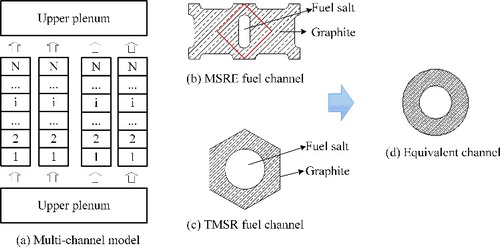
As left illustration (a) in Figure 3, the MSR filled with several parallel fuel channels is analyzed in this research, and those fuel channels are constructed by graphite in different ways shown as (b) and (c): MSRE fuel channel and TMSR fuel channel. In MSRE, groove is excavated in four sides of rectangular graphite assembly and two adjacent assemblies form one fuel channel [5]. On the contrary, one hole is excavated in each hexagonal graphite assembly in TMSR [16]. In the TH calculations, those two types of fuel channel are all approximated to a cylinder graphite with central cylinder fuel channel by equivalent hydraulic diameter [25] shown as (d) in Figure 3.

Figure 3. Multi-channel flow scheme and fuel channel geometry approximation along x–y direction.

The time-dependent mass balance equation, energy balance equation and momentum balance equation are solved by using the finite difference method for the spatial discretization. The Backward Euler method is applied for the time discretization by assuming uniform power density in each fuel channel and graphite segment. The feedback considering the average fuel and graphite temperature in each region is considered by interpolating the cross section.

In the steady-state case, the discretization scheme for Equations (22)(22) $$\begin{array}{c}\hfill \frac{\partial }{\partial t}\left(\rho \right)+\frac{\partial }{\partial z}\left(\rho v\right)=0\end{array}$$(22) through (24(24) $$\begin{array}{c}\hfill \frac{\partial }{\partial t}\left(\rho v\right)+\frac{\partial }{\partial z}\left(\rho v^2\right)+\frac{\partial P_{fric}}{\partial z}+g\rho +\frac{\partial P}{\partial z}=0\end{array}$$(24) ) are solved by coupling all with the same pressure drop in different fuel channels. The fuel temperature is then used as the boundary condition for the heat conduction in graphite. In the transient calculation, Equation (23) is first solved by using the flow distribution from the previous time step. The fuel salt temperature is calculated with the updated power at current time step. Iterations are performed to consider the updated hydraulic parameters. Then, the momentum and mass equation are solved by using the new fuel salt temperature. Also, the iterations are performed to converge the mass flow calculation by employing the same pressure drop in different fuel channels. Once the fuel temperature in each mesh is obtained, the radial dependent graphite temperature is obtained by using the effective heat transfer coefficients for the heat conduction equation in graphite [10].

2.7. Coupling scheme

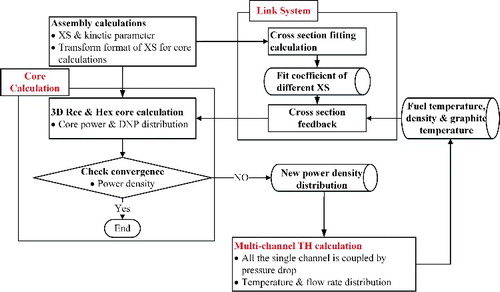
The overall iteration scheme of MOREL2.0 code is described in Figure 4. Three parts including the core calculation, cross-section interpolation and TH calculation are newly developed.

Figure 4. Calculation scheme for steady-state and transient-state calculation.

3. Numerical tests and code validation

3.1. Comparisons between MOREL and MOREL2.0

The TMSR project was proposed by Shanghai Institute of Applied Physics in China considering and TMSR is a 10-MWth thermal reactor moderated by graphite [16]. In this paper, a simplified TMSR model is established to compare the MOREL and MOREL2.0 codes. The geometry and core configuration is almost the same as that described in the previous paper [16]. Simplifications include taking away the fuel outlet in upper reflector and the control rods inside the core. Calculations are performed for both steady state and transient state. In the steady-state case, the eigenvalue, power density distribution and computational time are compared. The results are shown in Tables 1 and 2 and Figure 5. Table 1 shows that iteration number and computational time of MOREL2.0 are less than MOREL in eigenvalue calculation and that k-eff error of both two codes are all about 20 pcm in comparison with reference result. Average error E_aver, maximum error E_max and mean square error E_s for power distribution shown in Table 2 is defined as: (28) $$\begin{array}{c}\hfill E_{\mathrm{aver}}=\frac{{\sum }_{n=1}^N\left|P_n-P_{n,\mathrm{ref}}\right|}{N}\end{array}$$(28) (29) $$\begin{array}{c}\hfill E_{max}=max\left(\left|P_n-P_{n,\mathrm{ref}}\right|,n=1,2,...,N\right)\end{array}$$(29) (30) $$\begin{array}{c}\hfill E_s=\frac{\sqrt{{\sum }_{n=1}^N{\left|P_n-P_{n,\mathrm{ref}}\right|}^2}}{N}\end{array}$$(30) where P_n is nth assembly normalized power density; P_{n, ref} is nth assembly reference normalized power density; N is the total number of assembly.

Table 1. Comparison of eigenvalue, iteration number and computational time between MOREL and MOREL2.0 in steady-state case.

		Error	Iteration	Computational
Code	k-eff	(pcm)	number	time (s)
CITATION	1.10254	∼	∼	∼
MOREL	1.10274	20.0	1642	32.3
MOREL2.0	1.10275	21.0	13	19.5

Table 2. Power error of MOREL and MOREL2.0 by comparison with reference result in steady-state case.

Code	Average error (%)	Maximum error (%)	Mean square error (%)
MOREL	2.2279E-01	7.7969E-01	2.5590E-02
MOREL2.0	2.1045E-01	7.3981E-01	2.4333E-02

Figure 5. Normalized power density distribution compared between MOREL, MOREL2.0 and CITATION at steady state.

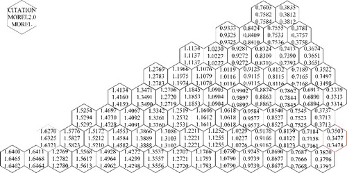
Table 2 shows that E_aver, E_max and E_s of both MOREL2.0 and MOREL are very close, which means two codes have the same accuracy. Those comparisons in Tables 1 and 2 present that accuracy of MOREL2.0 is the same with MOREL but MOREL2. 0 has better convergence and efficiency performance than MOREL.

In the transient case, a transient process for 5 s is simulated. The relative power variation and computational time are compared in Figure 6 and Table 3, respectively. Since different methods are applied in MOREL and MOREL2.0 for the time discretization, different time steps are used in the calculation. For MOREL, the time step of 0.01s is employed to ensure the accuracy. For MOREL2.0, two coarse time steps are performed and each of them is divided into 100 fine time steps. By the comparisons in Figure 6, MOREL2.0 shows good agreement with MOREL. Compared with the long computational time in MOREL calculation, MOREL2.0 reduces the computational cost by 2 orders of magnitude when adopting 1.0 s coarse time step.

Figure 6. Comparison of relative power variation for MOREL and MOREL2.0.

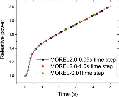
Table 3. Computational time comparison for MOREL and MOREL2.0 in transient state case.

Code	Time step (s)	Computational time (min)
MOREL	0.01	312.3
MOREL2.0	0.05	39.9
MOREL2.0	1.00	3

3.2. Code validation in comparison with experiment

The experimental data from published MSRE research report [5] is used to validate the newly updated MOREL2.0 code. The MSRE reactor is an 8-MWth liquid-fuel test reactor. The molten fluoride with temperature 922 K circulates through the graphite bar and leaves the core from the top plenum. The specification of reactor core is shown in Figure 7(a), and it is composed of 618 square stringers with the dimension of 5 cm × 5 cm × 170 cm. Four grooves are excavated in radial side of rectangular graphite assembly and two adjacent assemblies form one fuel channel as shown central top illustrations (b) in Figure 3. The moderator is graphite. The computational model is also depicted in Figure 7(b,c) with some simplification. Parts of the experimental data and TH parameters are listed in Tables 4 and 5, respectively [26,27].

Figure 7. MSRE experimental core (a) and reconstruction of MSRE core axial (b) and radial (c) cut.

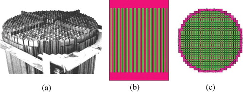
Table 4. Basic data of MSRE experimental test reactor from ORNL report.

Parameter	Value
Core diameter (m)	1.39
Core height(m)	1.63
Top and bottom plenum height (m)	0.1715
No. of square of stringers	618
Pitch of square of stringers (cm)	5.04
U235 enrichment	93%
Molar composition of fuel salt	LiF-BeF2-ZrF4--UF4 65%–29.1%–5.0%–0.9%
Total core power (MW)	8

Table 5. Thermal hydraulic parameters adopted in the MSRE simulation.

TH Parameter		Correlation/Value
The inlet fuel salt temperature (K)		908
Fuel Salt Density (g/cm^3)		ρsalt = 2.263 × (1 − 2.12 × 10^− 4 × (T(K) − 923))
Salt specific heat capacity (J/kg·K)		1868.0
Salt thermal conductivity (W/m·K)		1.4
Graphite Density (g/cm^3)		1.86
Graphite specific heat capacity (J/kg·K)		1757.3
Graphite thermal conductivity (W/m·K)		40.1
friction coefficient	Re ⩽ 2000	$f=64/\phantom{64Re}Re$
	2000 < Re ⩽ 2300	f = 0.048
	Re > 2300	$f=4\left(0.079/\phantom{0.079R{e}^{0.25}}R{e}^{0.25}\right)$
Nusselt number	Re ⩽ 2300	Nu = 4.36
	Re > 2300	Nu= 0.023Re^0.8Pr^0.4

The data collected in the European project MOST [28] are analyzed in this paper to validate the code. The data include:

1.	The loss of DNP in steady state at zero power
2.	Protected fuel pump start-up at zero power
3.	Protected fuel pump coast-down at zero power
4.	Fuel salt and graphite temperature distribution of the hottest channel at nominal power steady-state operation
5.	Fuel salt and graphite temperature coefficients and k-eff for MSRE
6.	Natural circulation simulation

The first three cases have already been simulated in the previous MOREL code. Thus, the results from both MOREL and MOREL2.0 are listed for comparison. Only MOREL2.0 can give the results for the later three cases by the fact that it requires coupling the TH calculation with the kinetics calculation.

3.2.1. The loss of DNP at steady-state operation

In MSR system, part of the DNP flow along with fuel circulation and decay outside the reactor core. As a result, the effective delayed neutron fraction β_eff is reduced. Consequently, the effective delayed neutron fraction for family i is defined as Equation (31)(31) $$\begin{array}{c}\hfill {\beta }_{\mathrm{eff}}^i=\frac{{\sum }_{g=1}^G{\int }_V{\varphi }_g^{*}\left(r\right){\chi }_{i,g}^d{\lambda }_i{C}_i\left(r\right)dv}{{\sum }_{g=1}^G{\int }_V{\varphi }_g^{*}\left(r\right){\chi }_{i,g}^d{\lambda }_i{C}_i\left(r\right)dv+\left(1-\beta \right){\sum }_{g=1}^G{\sum }_{g^{\text{'}}=1}^G{\int }_V{\varphi }_g^{*}\left(r\right){\chi }_g^p{\left(\nu {\Sigma }_f\right)}_{g^{\text{'}}}{\varphi }_{g^{\text{'}}}\left(r\right)dv}\end{array}$$(31) by introducing the ratio between total importance of delayed emissions from family i and total importance of all fission neutrons [5]. (31) $$\begin{array}{c}\hfill {\beta }_{\mathrm{eff}}^i=\frac{{\sum }_{g=1}^G{\int }_V{\varphi }_g^{*}\left(r\right){\chi }_{i,g}^d{\lambda }_i{C}_i\left(r\right)dv}{{\sum }_{g=1}^G{\int }_V{\varphi }_g^{*}\left(r\right){\chi }_{i,g}^d{\lambda }_i{C}_i\left(r\right)dv+\left(1-\beta \right){\sum }_{g=1}^G{\sum }_{g^{\text{'}}=1}^G{\int }_V{\varphi }_g^{*}\left(r\right){\chi }_g^p{\left(\nu {\Sigma }_f\right)}_{g^{\text{'}}}{\varphi }_{g^{\text{'}}}\left(r\right)dv}\end{array}$$(31) where standard notations of neutronics are used; V is all computational space; ϕ* is adjoint flux.

The loss of effective delayed neutron fraction β_loss is defined as: (32) $$\begin{array}{c}\hfill {\beta }_{\mathrm{loss}}=\sum _i{\beta }_{\mathrm{eff}}^{i,\mathrm{static}}-\sum _i{\beta }_{\mathrm{eff}}^{i,flow}\end{array}$$(32) where β^{i, static}_eff and β^{i, flow}_eff are the effective delayed neutron fraction of family i when the fuel velocity is neglected and considered, respectively

The loss of delayed neutron fraction β_loss for each DNP family is calculated for both U235 and U233 fuels in this paper. Comparison of MOREL2.0 results, MSRE experimental values and the other calculation results [29] are listed in Tables 6 and 7. FZK participates with two codes, SIMMER and SimADS: results are identified in the following with (a) and (b), respectively. MSRE and ORNL are the experimental values of MSRE and the results of calculations performed by ORNL, respectively.

Table 6. Loss of delayed neutron fraction (pcm) in steady-state operation for U-235 fuel.

	Total	Family 1	Family 2	Family 3	Family 4	Family 5	Family 6
MSRE	212
ORNL	222
BUTE	244
EDF	228.8	12.0	78.0	62.3	73.7	2.8	0.0
ENEA	259.2	14.0	90.5	71.1	80.4	3.2	0.1
FZK^a	262.2	14.1	90.8	70.9	81.9	4.1	0.3
FZK^b	212.2	12.6	77.5	52.8	62.4	5.6	0.9
FZR	253.2	13.8	89.2	68.4	77.8	3.9	0.1
POLITO	278.0	16.0	100.7	74.1	82.8	4.0	0.2
MOREL	246.3	13.6	88.8	67.7	73.6	2.5	0.0
MOREL2.0	260.2	18.5	106.8	67.3	64.8	2.5	0.0

^a Using the SIMMER code.

^b Using the SimADS code.

MSRE – the experimental data; ORNL – the numerical results from ORNL.

Table 7. Loss of delayed neutron fraction (pcm) in steady-state operation for U-233 fuel.

	Total	Family 1	Family 2	Family 3	Family 4	Family 5	Family 6
MSRE	100.5
ORNL	100.5	12.4	43.9	28.2	15.6	0.4	0.1
BUTE	85
EDF	107.8	12.4	44.1	30.8	20.0	0.5	0.0
ENEA	122.4	14.4	51.4	34.7	21.5	0.5	0.0
FZK^a	125.0	14.5	51.7	35.1	22.7	0.8	0.1
FZK^b	105.4	13.6	45.1	26.7	18.4	1.2	0.3
FZR	121.0	14.3	50.6	33.6	21.2	1.4	0.0
POLITO	134.5	16.7	57.7	36.3	22.9	0.8	0.1
MOERL	102.2	13.5	38.2	24.0	26.1	0.7	0.0
MOREL2.0	109.2	18.2	41.6	23.0	25.1	1.1	0.1

^aUsing the SIMMER code.

^bUsing the SimADS code.

MSRE – the experimental data; ORNL – the numerical results from ORNL.

The total β_loss calculated by the MOREL2.0 code is 260.2 and 109.2 pcm for the U235 fuel and U233 fuel, respectively. The results from MOREL and MOREL2.0 have slight differences due to the different diffusion equation solver, whole calculation scheme, but the difference between MOREL and MOREL2.0 is 13.9 and 7 pcm for U235 fuel and U233 fuel, respectively. The results calculated by both MOREL and MOREL2.0 are close to experiment data and other calculation results.

However, some differences between the numerical results and the experimental data can be found. For most codes, the calculated results are higher than the experimental data. The difference may come from the simplification of core geometry and different models used for evaluating the loss of delayed neutron importance.

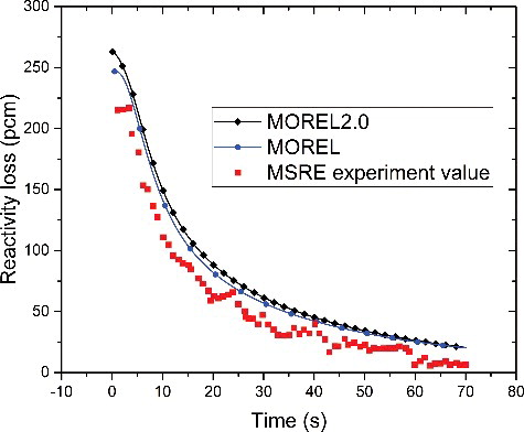
3.2.2. Reactivity loss at protected fuel pump coast-up and coast-down

DNP redistribution caused by fuel circulation lead core reactivity loss which has the same value with β_loss. As for the protected transient cases, the zero power and criticality are maintained by adjusting the control rods. In the MOREL2.0 calculations, the TH parameters are simulated by using the given inlet fuel flow depicted in Figure 8 [27]. The inlet fuel flow increases from zero to the nominal value at the start of 10 seconds for the pump start-up case. In the pump coast-down case, the fuel flow decreases from the nominal values to zero at the start of 20 seconds. The results of reactivity loss are compared in Figures 9 and 10. In the previous MOREL calculations, the uniform fuel velocity and temperature were employed. From the comparison results in Figures 9 and 10, reactivity loss calculated by MOREL2.0 and MOREL are close to each other and the maximum error between two codes is 10.1 pcm, and the calculation results of both MOREL2.0 and MOREL show good agreement with the experiment data but some differences in the amplitude of oscillations can be observed. This is probably due to the using of simplified MSRE model in MOREL2.0 calculation and a limitation on the control rods’ withdrawal speed in MSRE experiment [29].

Figure 8. MSRE inlet fuel flow curve during transient of fuel pump start-up (square) and coast-down (diamond).

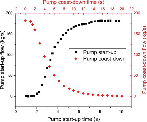
Figure 9. Reactivity compensation during the transient of pump start-up.

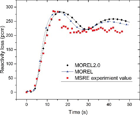
Figure 10. Reactivity compensation during the transient of pump coast-down.

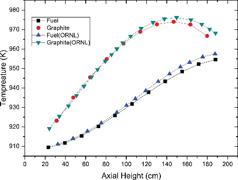
3.2.3. Neutronics and TH verification at MSRE steady state

The steady operation of MSRE with nominal power is simulated. The temperature distribution of fuel and graphite in the hottest channel is shown in Figure 11. The experimental data labeled ORNL in Figure 11 serves as the reference [30]. The numerical results show good agreement and the maximum relative error is less than 1%.

Figure 11. Fuel salt and graphite temperature distribution in the hottest channel.

Another case is calculated for the multiplication factor and reactivity coefficients of the fuel salt and graphite. In this case, the uniform fuel and graphite temperature of 923 K is adopted. The calculation results are listed in Table 8, where MSRE and ORNL indicate the experiment values of MSRE and calculation results performed by ORNL [29]. It shows that the accuracy of MOREL2.0 code is similar to the other MSR codes and the MSRE model established in this paper is appropriate for the further simulation.

Table 8. Fuel salt and graphite temperature coefficients and effective multiplication factor for MSRE.

	Institute	K-eff	Salt coefficient	Graphite coefficient	Total coefficient
U235 Fuel	MSRE		−8.5	−4.7	−13.2
	ORNL		−7.5	−7.3	−14.8
	BUTE	1.0598	−6.2	−4.8	−11.0
	ENEA	1.07513	−6.8	−4.3	−11.1
	EDF	1.06752	−7.8	−4.6	−12.4
	FZR	1.06966	−6.9	−4.0	−10.9
	POLITO	1.07060	−6.3	−3.8	−10.1
	MOREL2.0	1.06643	−7.4	−4.5	−11.9

3.2.4. Natural circulation simulation

In the MSRE experiments, the natural convection was driven by the secondary circuit, whose cooling capacity was step-wise increased [28]. The calculation is performed based on the MOST benchmark rather than the experimental report [29]. The aim of this benchmark is to compare the reactor power response. For this response calculation, the fuel salt and graphite temperature feedback coefficients are important, and these coefficients have been calculated and compared in Table 8.

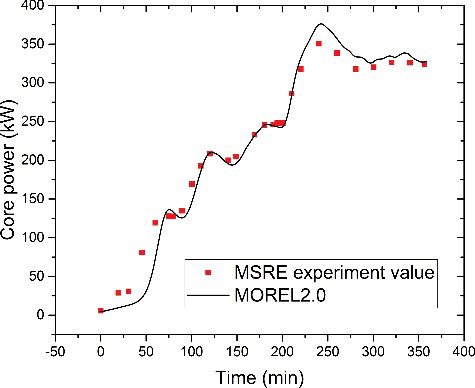
At the beginning of transient, the reactor power is stabilized at 4.1 kW with the limited fuel mass flow rate. The inlet fuel temperature is 898 K. The transient process is illustrated in Figure 12, where inlet mass flow is referred to [27] because there is no experiment data on mass flow in natural circulation. The comparison of power response during the natural circulation is shown in Figure 13. The results are in good agreement with the experimental data. In particular, different behavior at the start of transient can be noticed. It is due to the fact that the reactor is probably not in the ideal equilibrium state, which is assumed in the calculations [29].

Figure 12. Fuel mass flow rate and fuel inlet temperature calculated by MOST benchmark.

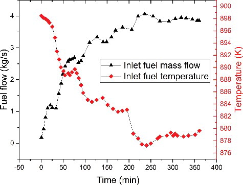
Figure 13. Power history during 360 minutes of the natural circulation experiment and comparison with the experiment results.

4. Conclusion

In this paper, the MOREL code dedicated for the MSRE analysis is updated to MOREL2.0. The new features in MOREL2.0 includes: (1) employing the PCIQS method for the kinetics model of liquid fuel in MSR, (2) coupling the multi-channel TH model to the neutronics calculation, and (3) using the VNM nodal method to solve the neutron diffusion equation.

Numerical tests have been done to assess the new MOREL2.0 code. The results prove that the new code has the same accuracy with the previous one. By using the new methods, the efficiency is significantly improved. For the steady-state calculation, the speed-up ratio is around 2. And, for the transient calculation, the computational time is reduced by 2 orders of magnitude.

By coupling with the TH calculation, the updated MOREL2.0 code is capable of doing the real transient core analysis. The experiments of MSRE are simulated to validate the code. The results from other MSR codes and the data gained from the MSRE experiments are compared. It is proved that the new code is capable of accurately modeling and simulating an MSR using the liquid fuel.

Acknowledgements

This work is financially supported by the National Science Foundation of China [grant numbers 11522544, 91226106]. The MSRE experimental data used in the article are referred to the MSRE operation reports of Oak Ridge National Laboratory

Disclosure statement

No potential conflict of interest was reported by the authors.

Additional information

Funding

National Science Foundation

References

- Pioro IL. Handbook of generation IV nuclear reactors. Cambridge (UK): Woodhead Publishing; 2016.
- John EK. Generation IV international forum: a decade of progress through international cooperation. Prog Nucl Energy. 2014;77:240–246.
- Abram T, Ion S. Generation-IV nuclear power: a review of the state of the science. Energy Policy. 2008;36:4323–4330.
- Haubenreich PN, Engel JR, Prince BE, et al. MSRE design and operations report, part III, nuclear analysis. Oak Ridge (TN): Oak Ridge National Laboratory; 1964. ( ORNL-TM-730).
- Hugo VD. Delayed neutron effectiveness in a fluidized bed fission reactor. Ann Nucl Energy. 1996;23:41–46.
- Kophazi J, Szieberth M, Feher S. MCNP-based calculation of reactivity loss in circulating fuel reactors. Proceedings of the International Conference on Nuclear Mathematical and Computational Sciences: A Century in Review-A Century Anew; 2003 April 6–10; Gatlinburg, TN.
- Serp J, Allibert M, Beneš O, et al. The molten salt reactor (MSR) in generation IV: overview and perspectives. Prog Nucl Energy. 2014;77:308–319.
- Wang S, Rineiski A, Maschek W. Molten salt related extensions of the SIMMER-III code and its application for a burner reactor. Nucl Eng Des. 2006;236:1580–1588.
- Křepel U, Grundmann J, Rohde U, et al. DYN1D MSR dynamics code for molten salt reactors. Ann Nucl Energy. 2005;32:1799–1824.
- Křepel J, Rohde U, Grundmann U, et al. DYN3D MSR spatial dynamics code for molten salt reactors. Ann Nucl Energy. 2007;34:449–462.
- Lecarpentier D, Carpentier V. A neutronics program for critical and nonequilibrium study of mobile fuel reactors: the Cinsf1D code. Nucl Sci Eng. 2003;143:33–46.
- Guo ZP, Zhou JJ, Zhang DL, et al. Coupled neutronics/thermal-hydraulics for analysis of molten salt reactor. Nucl Eng Des. 2013;258:144–156.
- Dulla S, Ravetto P, Rostagno MM. Neutron kinetics of fluid-fuel systems by the quasi-static method. Ann Nucl Energy. 2004;31:1709–1733.
- Zhang DL, Qiu SZ, Su GH, et al. Development of a steady state analysis code for a molten salt reactor. Ann Nucl Energy. 2009;36:590–603.
- Zhang DL, Qiu SZ, Su GH, et al. Analysis on the neutron kinetics for a molten salt reactor. Prog Nucl Energy. 2009; 51:624–636.
- Zhuang K, Cao LZ, Zheng YQ, et al. Studies on the molten salt reactor: code development and neutronics analysis of MSRE-type design. Nucl Sci Technol. 2014; 52:251–263.
- Li YZ. Advanced reactor core neutronics computational algorithms based on the variational nodal and nodal SP3 methods [Doctoral dissertation]. Xi'an (China): Xi'an Jiaotong University; 2012.
- Stamm'ler RJJ. HELIOS methods. In: Program manual rev. 3, program HELIOS-1.5. Waltham (MA): Studsvik Scandpower; 1998. p. IX–1.
- Shim CB, Jung YS, Joo HG, et al. Application of backward differentiation formula to spatial reactor kinetics calculation with adaptive time step control. Nucl Eng Technol. 2011; 43(6):531–546.
- Hoffman A. A time-dependent method of characteristics formulation with time derivative propagation [Doctoral dissertation]. Ann Arbor (MI): University of Michigan; 2013.
- Henry AF. Nuclear-reactor analysis. Cambridge (MA): MIT Press; 1975.
- Akcasu Z, Lellouche GS, Shotkin LM. Mathematical methods in nuclear reactor dynamics. New York (NY): Academic Press; 1971.
- Lapenta G, Ravetto P, Ritter G. Effective delayed neutron fraction for fluid-fuel systems. Ann Nucl Energy 2000;27:1523–1532.
- Dulla S, Mund E, Ravetto P. The quasi-static method revisited. Prog Nucl Energy 2008; 50:908–920.
- Hu TL, Wu HC, Cao LZ, et al. [Neutronics and thermal-hydraulics coupling analysis of molten salt reactor at steady state]. At Energy Sci Technol. 2016;50:1823–1827. Chinese.
- Prince VE, Ball SJ, Engel JR. Zero-power physics experiments on molten-salt reactor experiment. Oak Ridge (TN): Oak Ridge National Laboratory; 1968. ( ORNL-4233).
- Křepel J. Dynamics of molten salt reactors [Doctoral dissertation]. Prague (Czech Republic): Czech Technical University in Prague; 2006.
- Rosenthal MW. Molten-salt reactor program semi-annual progress report for period ending February 28 1969. Oak Ridge (TN): Oak Ridge National Laboratory; 1969. ( ORNL-4396).
- Delpech M, Dulla S, Garzenne C, et al. Benchmark of dynamic simulation tools for molten salt reactors. International Conference GLOBAL 2003; 2003 Nov; New Orleans, LA.
- Engel JR, Haubenreich PN. Temperature in the MSRE core during steady-state power operation. Oak Ridge (TN): Oak Ridge National Laboratory; 1962. ( ORNL-TM-378).