Application of dynamical system scaling method on simple gravity-driven draining process

ABSTRACT

Scaling analysis is widely used in the design of nuclear reactor passive safety systems to ensure that the scale-down test facilities can accurately capture the important phenomena in the prototypic system. In this study, the scaling distortion of a gravity-driven draining system has been analyzed with Hierarchical Two-Tiered Scaling (H2TS) method, based on the initial static characteristic values. In the draining process, however, the key parameters may vary with respect to time, leading to a certain level of scaling distortion. To evaluate the time-dependent scaling distortion, a Dynamical System Scaling (DSS) method is applied. Through comparisons of scaling results of the two scaling methods, it is concluded that the H2TS method can effectively scale the gravity-driven draining process in different geometric sizes, if the variations in the friction factor is negligible. As the draining process slows down, accompanied by an increase in the friction factor, the distortions in water level and in discharge velocity become significant, especially at the end of the draining process in a model of relatively small geometry size. This preliminary study demonstrated the process of scaling distortion analysis using the DSS identity method, and could shed light to the scaling distortion evaluation of testing programs.

KEYWORDS:

• DSS
• gravity-driven draining
• scaling distortion

1. Introduction

In recent years, the passive technology has been widely used in many industrial fields, especially in the third generation nuclear power plant design such as AP1000 [1]. Further advancement of larger pressurized water reactors like CAP1700 (with the electric power of 1700 MW), one of the Chinese National Science & Technology major projects, is in progress, based on the AP1000 passive technology [2]. The nuclear safety can be dramatically improved by adopting typical passive systems, such as the passive core cooling system and the passive containment cooling system. Here, gravity plays a key role in some accidental events. For example, the passive core makeup tank (CMT) injects the emergency coolant to the reactor core using gravitational potential in case of small-break loss of coolant accident (LOCA) as it is installed at a higher location than that of the reactor core. Thus, it is of great significance to deeply understand the mechanism of gravity-driven draining in CMT system in a comprehensive manner.

Research has been done on the gravity-driven draining process in CMT system mainly by means of experiments and numerical simulation. Sang and Hee made a gravity-driven injection experiment by using a small-scale test facility to identify the parameters affecting the gravity-driven injection, finding that the water subcooling affected greatly on the injection initiation [3]. Ji et al. also carried out experiments to investigate the gravity-draining process based on a small-scale water tank model for the AC600 Pressurized Water Reactor [4]. Peng did CMT draining experiments and the results showed that the fluid temperature distribution and the pressure response in the CMT are dependent on the initial temperature of the CMT [5]. Liao and Zhou studied the dynamic relationship between the driving force and the friction under certain accidental conditions using Relap5 code [6]. Wang et al. simulated the CMT system of China's Pressurized Water Reactor using Relap5 code based on the prototype size, showing that the CMT can effectively provide emergency core cooling [7].

The above studies revealed many useful principles on the CMT draining process. However, no detailed scaling analysis has been carried out for these experiments and simulations. The corresponding scaling analysis is essential to ensure the scale-down test facilities can accurately capture the important phenomena in the prototypic system. Several integral thermal–hydraulic test facilities consisting of the CMT component have been built to validate the performance of the passive systems used in the Generation III reactors by means of systematic scaling analysis. Yonomoto et al. conducted several integral experiments to simulate small-break LOCA utilizing the ROSA-V large-scale test facility. They concluded that the drain rates are predicted well by only considering the liquid head in the CMT and flow resistance in the discharge line after the pressure balance line is empty of liquid [8–9]. The CMT in the SPES-2 test facility with full height and full pressure is adopted as a double-shell structure in order to reduce the scaling distortion on the gravity-driven draining process [10]. On the other hand, the APEX test facility is designed with low pressure and scale-down height, which can ensure lower scaling distortion during the steam condensation in the CMT, while the draining stage under high pressure condition cannot be reproduced very well due to different system pressure [11–12]. The newly built Advanced Cooling Mechanism Experiment test facility is also an integral one with high pressure and scale-down height, which can provide validating data for China's advanced nuclear power plant CAP1400. However, a certain degree of scaling distortion still occurs in the CMT draining process due to the deviation of steam condensation [13].

Most of the above mentioned integral test facilities are designed based on the typical Hierarchical Two-Tiered Scaling (H2TS) method [14], which has been widely adopted in nuclear industry. Note that in these experiments, the characteristic parameters used for the similarity criteria are the initial values or the steady-state values. Moreover, the evaluation on the scaling distortion is also static. However, in the dynamic process such as the gravity-driven draining, the key parameters may vary with respect to time, leading to a certain level of scaling distortion. It is therefore not appropriate to evaluate a dynamic system using static parameters. In order to quantitatively assess this dynamic scaling distortion, Reyes developed a new DSS (Dynamical system scaling) method to optimize the system scaling and evaluate the scaling distortion produced in the entire transient process [15]. This method describes the physical processes as geometric objects in a normalized coordinate system and can show how the time-dependent distortion between prototype and scaled model processes can be compared quantitatively. In this paper, the DSS identity method is introduced into a simple gravity-driven draining process, and the results are compared with that obtained from the H2TS method, especially the dynamic deviation.

2. DSS methodology [15]

The integral balance equation described by Reyes is as follows: (1) $$\begin{array}{c}\hfill \frac{d}{dt}\left\{\int \int \int \psi \left(t\right)dV\right\}=\sum _{i=1}^n{\varphi }_i\end{array}$$(1) where ψ(t) is the instantaneous amount of space-integrated conserved quantity in the continuity equation, and ϕ_i is the i-agent-of-change acting to change the conserved quantity.

Defining the normalized conserved quantity as (2) $$\begin{array}{c}\hfill \beta \left(t\right)=\frac{\psi \left(t\right)}{{\psi }_0}\end{array}$$(2) where ψ₀ is a time-independent value of the integrated conserved quantity for the process.

The normalized sum of agents-of-change is defined as (3) $$\begin{array}{c}\hfill \omega \left(t\right)=\frac{1}{{\psi }_0}\sum _{i=1}^n{\varphi }_i=\sum _{i=1}^n\frac{{\varphi }_i}{{\psi }_0}\end{array}$$(3)

Substituting Equations (2)(2) $$\begin{array}{c}\hfill \beta \left(t\right)=\frac{\psi \left(t\right)}{{\psi }_0}\end{array}$$(2) and (3(3) $$\begin{array}{c}\hfill \omega \left(t\right)=\frac{1}{{\psi }_0}\sum _{i=1}^n{\varphi }_i=\sum _{i=1}^n\frac{{\varphi }_i}{{\psi }_0}\end{array}$$(3) ) into Equation (1)(1) $$\begin{array}{c}\hfill \frac{d}{dt}\left\{\int \int \int \psi \left(t\right)dV\right\}=\sum _{i=1}^n{\varphi }_i\end{array}$$(1) yields the integral balance equation: (4) $$\begin{array}{c}\hfill \frac{d\beta }{dt}=\omega \end{array}$$(4)

The process time is defined as follows: (5) $$\begin{array}{c}\hfill \tau =\frac{\beta }{\omega }\end{array}$$(5)

Differentiate the process time to the reference time, (6) $$\begin{array}{c}\hfill d\tau =(1+D)dt\end{array}$$(6)

D is the temporal displacement rate: (7) $$\begin{array}{c}\hfill D=-\frac{\beta }{{\left(\omega \right)}^2}\frac{d\omega }{dt}\end{array}$$(7)

The process time interval is obtained by integrating Equation (6)(6) $$\begin{array}{c}\hfill d\tau =(1+D)dt\end{array}$$(6) : (8) $$\begin{array}{c}\hfill {\tau }_s={\tau }_2-{\tau }_1={\int }_{t_1}^{t_2}(1+D)dt\end{array}$$(8)

The normalized coordinates and parameters are defined as (9) $$\begin{array}{c}\hfill \tilde{\Omega }=\omega {\tau }_s,\tilde{\beta }=\beta ,\tilde{t}=t/{\tau }_s,\tilde{\tau }=\tau /{\tau }_s\end{array}$$(9)

Based on identity transformation law [15], the similarity criteria are obtained as follows: (10) $$\begin{array}{c}\hfill {\tilde{\Omega }}_R=1,{\beta }_R=1,{\omega }_R=1,{\tau }_R=t_R=1\end{array}$$(10)

3. Modeling simple gravity-driven draining system

3.1. Assumptions

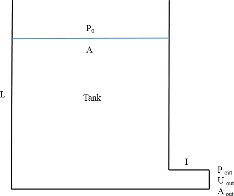
A simple water tank model is built as shown in Figure 1. The scaling analysis is performed based on several simplifying assumptions, which are given as follows:

(1)	One-dimensional flow: the fluid only flows along the axis of the tank and the pipe;
(2)	Both the top of the tank and the pipe exit are open to the atmosphere, that is, P0 = Pout;
(3)	The volume of the pipe is negligible since it is very small compared with that of the tank.

Figure 1. Sketch of gravity-driven draining system.

3.2. Conservation equations and simplified dimensionless forms

3.2.1. Continuity equation

(11) $$\begin{array}{c}\hfill \frac{\partial \rho V}{\partial t}=-W_{\mathrm{out}}\end{array}$$(11) where W_out is the mass flow rate, ρ is the fluid density, V is the fluid volume, and t is the time.

Define the characteristics time. (12) $$\begin{array}{c}\hfill {\tau }_0=\frac{m_0}{W_{\mathrm{out},0}}=\frac{\rho L_{0}A}{\rho A_{\mathrm{out}}{u}_{\mathrm{out}0}}\end{array}$$(12) where m₀ is the initial fluid quality in the tank, L₀ is the initial water level in the tank, A is the cross-section area of the tank, A_out is the cross-section area of the pipe, and u_out0 is the initial discharge velocity at the pipe exit.

Define the following parameters: L⁺ = L/L₀, t⁺ = t/τ₀, u⁺_out = u_out/u_out0, then the dimensionless equation can be obtained: (13) $$\begin{array}{c}\hfill \frac{d{L}^{+}}{d{t}^{+}}=-u_{\mathrm{out}}^{+}\end{array}$$(13)

3.2.2. Energy equation

(14) $$\begin{array}{ccc}\hfill P_0+\frac{1}{2}\rho u^2+\rho gL\left(t\right)& =& P_{\mathrm{out}}+\frac{1}{2}\rho u_{\mathrm{out}}^2+\rho g{L}_{\mathrm{out}}\hfill \\ & & +(\frac{fl}{d}+k)\frac{1}{2}\rho u_{\mathrm{out}}^2\hfill \end{array}$$(14) where u is the velocity in the tank, d is the diameter of the pipe, set L_out = 0. It is clear that u ≪ u_out. Here, we define the energy loss coefficient $F_r=\frac{fl}{d}+k$. The above equation can be simplified as (15) $$\begin{array}{c}\hfill u_{\mathrm{out}}=\sqrt{\frac{2gL\left(t\right)}{1+F_r}}\end{array}$$(15)

Ignore the effect of the fluid velocity on the energy loss coefficient, then: (16) $$\begin{array}{c}\hfill u_{\mathrm{out}}^{+}={\left(L^{+}\right)}^{1/2}\end{array}$$(16)

It can be concluded that the phenomenon similarity between the prototype and the model can be guaranteed automatically as long as the geometry similarity is satisfied.

Substitute (15(15) $$\begin{array}{c}\hfill u_{\mathrm{out}}=\sqrt{\frac{2gL\left(t\right)}{1+F_r}}\end{array}$$(15) ) into (11(11) $$\begin{array}{c}\hfill \frac{\partial \rho V}{\partial t}=-W_{\mathrm{out}}\end{array}$$(11) ), (17) $$\begin{array}{c}\hfill \frac{dL\left(t\right)}{dt}=-\left(\frac{A_{\mathrm{out}}}{A}\right)\sqrt{\frac{2gL\left(t\right)}{1+F_r}}\end{array}$$(17)

Integrate the above equation and we can obtain the solution as follows: (18) $$\begin{array}{c}\hfill L\left(t\right)=(L_0^{1/2}-\frac{c}{2}t{)}^2\end{array}$$(18)

where $c=\left(\frac{A_{\mathrm{out}}}{A}\right)\sqrt{\frac{2g}{1+F_r}}$.

Dimensionless form: (19) $$\begin{array}{c}\hfill L^{+}=(1-\frac{1}{2}{t}^{+}{)}^2\end{array}$$(19)

Equation 19(19) $$\begin{array}{c}\hfill L^{+}=(1-\frac{1}{2}{t}^{+}{)}^2\end{array}$$(19) shows that the dimensionless water level is only related to dimensionless time.

The maximum process time can be obtained from Equation (19)(19) $$\begin{array}{c}\hfill L^{+}=(1-\frac{1}{2}{t}^{+}{)}^2\end{array}$$(19) : (20) $$\begin{array}{c}\hfill t_{max}=\frac{2\sqrt{L_0}}{c}=2{\tau }_0\end{array}$$(20)

The dimensionless process curve can be figured out based on Equations (16)(16) $$\begin{array}{c}\hfill u_{\mathrm{out}}^{+}={\left(L^{+}\right)}^{1/2}\end{array}$$(16) and (19(19) $$\begin{array}{c}\hfill L^{+}=(1-\frac{1}{2}{t}^{+}{)}^2\end{array}$$(19) ), as shown in Figure 2.

Figure 2. Dimensionless process curves.

It must be noted that the above analytical solutions are obtained only by assuming F_r as constant. Actually, F_r varies with time-dependent velocity, and there may be some scaling distortion if the scaling criteria are adopted based on the above simplified equations. For convenience of contrast, the similarity criteria with the H2TS method are summarized first, and then compared with that based on the DSS identity method.

3.3. Similarity criteria with H2TS method

Define X_R = X_m/X_p, where X represents any variable, the subscript R, m, p denote the ratio, model, and prototype, respectively. The similarity criteria based on the H2TS method can be readily obtained as follows:

(1)	Geometry similarity: (21) $$\begin{array}{c}\hfill L_{0,R}=D_R=l_R=d_R;\end{array}$$(21) (22) $$\begin{array}{c}\hfill A_R=A_{\mathrm{out},R}=L_{0,R}^2;\end{array}$$(22)
(2)	Fr is kept unchanged, which can be obtained by adjusting the form loss coefficient k, (23) $$\begin{array}{c}\hfill \\ \hfill {(1+F_r)}_R=1;\end{array}$$(23)
(3)	(24) $$\begin{array}{c}\hfill u_{\mathrm{out}0,R}=L_{0,R}^{1/2};\end{array}$$(24)
(4)	(25) $$\begin{array}{c}\hfill \\ \hfill {\tau }_R=L_{0,R}^{1/2};\end{array}$$(25)
(5)	(26) $$\begin{array}{c}\hfill W_{\mathrm{out}0,R}=L_{0,R}^{5/2}.\end{array}$$(26)

Figure 3 gives the length-dependent similarity parameter groups. It is clear that the two curves, which stand for u_{out0, R} and τ_R respectively, overlap.

Figure 3. Similarity parameter curve based on H2TS method.

3.4. Results and discussions based on H2TS method

For convenience of comparison, several typical cases with different scaling sizes are provided based on the H2TS method, as shown in Table 1. For the turbulent flow, the friction coefficient f can be calculated as $f=0.316{\mathrm{R}}_e^{-0.25}=0.316{(\rho ud/\mu )}^{-0.25}$. In addition, if the water temperature is set as 20 ^oC, and consider the local resistance loss in the outlet pipe (including two conditions, the cross-section decreasing and increasing sharply), then the value of F_r can be obtained.

Table 1. Comparison of different scaling parameters with H2TS method

Parameter	Scale 1/1	Scale 1/2	Scale 1/3	Scale 1/4	Scale 1/6
L0 (m)	9	4.5	3	2.25	1.5
D (m)	3	1.5	1	0.75	0.5
l (m)	2.1	1.05	0.7	0.525	0.35
d (m)	0.21	0.105	0.07	0.0525	0.035
Fr	1.5872	1.5872	1.5872	1.5872	1.5872
uout0	8.26	5.8407	4.7689	4.13	3.3721
c	0.01349	0.01349	0.01349	0.01349	0.01349
tmax	444.7284	314.4704	256.764	222.3642	181.5596
τ	222.3642	157.2352	128.382	111.1821	90.7798

Figures 4 and 5 show the time-dependent curve of the water level and the discharge velocity based on actual friction coefficient. It is obvious that all the curves almost overlap, except some deviation at the end of the processes. Similar curves can also be captured based on ideal friction coefficient. The following discussion will then be focused on the variation of water level since both the water level and velocity have identical variation tendency.

Figure 4. Time-dependent water level based on actual friction coefficient.

Figure 5. Time-dependent discharge velocity based on actual friction coefficient.

Figure 6 gives the time-dependent water level error between the analytical values and the actual ones. Here, the analytical values are calculated based on constant energy loss coefficient F_r, and the actual ones are obtained by considering the time-dependent F_r. The corresponding error is defined as follows: (27) $$\begin{array}{c}\hfill \mathrm{Error}=\frac{L_{\mathrm{analytical}}^{+}-L_{\mathrm{actual}}^{+}}{L_{\mathrm{actual}}^{+}}\times 100\%\end{array}$$(27)

Figure 6. Time-dependent water level error between the analytical values and the actual ones.

Similar characteristics are exhibited from these curves. First, the water level deviation under all cases increases with dimensionless time during the entire period. In the time range t⁺ = 0-1.5, the error increases gradually, which corresponds to 0%–5%. However, the deviation dramatically increases as t⁺ > 1.7. Second, the negative error means that the analytical water level is always less than the actual one. It is clear that this is due to the variation of the friction loss coefficient, as shown in Figure 7. All the actual friction coefficients are greater than the analytical ones and the corresponding curves behave as similar characteristics with those in Figure 6. Furthermore, the actual friction coefficient increases with decreasing scaling size. As a result, the water level deviation in Figure 6 increases monotonically with the decreasing scaling size.

Figure 7. Time-dependent friction coefficients.

Figure 8 shows the actual water level errors between the prototype and the model. Like in the previous curves, almost no deviation can be found in the first-half period. However, in the second-half period, the water level error increases gradually with decrease of the model geometry size, especially at the end of the processes. This is mainly because the water level has dropped to lower than the height of the outlet pipe (i. e. the outlet pipe diameter), resulting in the change of the flow loss coefficients. The calculated water level errors as the water level drops to the height of the outlet pipe are 2.76% (for the scale 1/2), 4.4% (for the scale 1/3), 4.72% (for the scale 1/4), 6.09% (for the scale 1/6), respectively, and all correspond to time t⁺ = 1.48. The remaining distortion is due to idealized estimation on the local resistance loss coefficient.

Figure 8. Time-dependent water level error based on actual values.

3.5. Similarity criteria with DSS identity method

Rewrite Equation (13)(13) $$\begin{array}{c}\hfill \frac{d{L}^{+}}{d{t}^{+}}=-u_{\mathrm{out}}^{+}\end{array}$$(13) as (28) $$\begin{array}{c}\hfill \frac{d{L}^{+}}{dt}=-\frac{1}{{\tau }_0}{u}_{\mathrm{out}}^{+}\end{array}$$(28)

According to the DSS method, define (29) $$\beta =L^{+}$$(29) (30) $$\omega =-\frac{1}{{\tau }_0}{u}_{\mathrm{out}}^{+}$$(30)

Rewriting Equation (7)(7) $$\begin{array}{c}\hfill D=-\frac{\beta }{{\left(\omega \right)}^2}\frac{d\omega }{dt}\end{array}$$(7) , the temporal displacement rate: (31) $$\begin{array}{c}\hfill D=-\frac{\beta }{{\left(\omega \right)}^2}\frac{d\omega }{dt}\end{array}$$(31)

Substitute Equations (29)(29) $$\beta =L^{+}$$(29) , (30(30) $$\omega =-\frac{1}{{\tau }_0}{u}_{\mathrm{out}}^{+}$$(30) ), (16(16) $$\begin{array}{c}\hfill u_{\mathrm{out}}^{+}={\left(L^{+}\right)}^{1/2}\end{array}$$(16) ), and (19(19) $$\begin{array}{c}\hfill L^{+}=(1-\frac{1}{2}{t}^{+}{)}^2\end{array}$$(19) ) into Equation (31)(31) $$\begin{array}{c}\hfill D=-\frac{\beta }{{\left(\omega \right)}^2}\frac{d\omega }{dt}\end{array}$$(31) , then (32) $$\begin{array}{c}\hfill D=-\frac{1}{2}\end{array}$$(32)

The process time interval:

(33) $$\begin{array}{c}\hfill {\tau }_s={\tau }_2-{\tau }_1={\int }_0^{t_{max}}(1+D)dt={\tau }_0\end{array}$$(33)

Here, according to the identity transformation law (more details can be seen in reference [15]), ${\tilde{\Omega }}_R=1,{\beta }_R=1,{\omega }_R=1,{\tau }_R=t_R=1$, it then can be obtained as follows: (34) $$L_{{}^R}^{+}=1$$(34) (35) $${\tau }_{0,R}=1$$(35)

Basically, assume the geometry similarity, then (36) $$L_{0,R}=D_R=l_R=d_R$$(36) (37) $$A_R=A_{\mathrm{out},R}=L_{0,R}^2$$(37)

Based on Equation (20)(20) $$\begin{array}{c}\hfill t_{max}=\frac{2\sqrt{L_0}}{c}=2{\tau }_0\end{array}$$(20) , substitute τ₀ into Equation (35)(34) $$L_{{}^R}^{+}=1$$(34) , $$\begin{array}{ccc}\hfill {\tau }_{0,R}& =& (\frac{\sqrt{L_0}}{c}{)}_R={\left(\frac{\sqrt{L_0}}{\left(\frac{A_{\mathrm{out}}}{A}\right)\sqrt{\frac{2g}{1+F_r}}}\right)}_R\hfill \\ & =& L_{0,R}^{1/2}{(1+F_r)}_R^{1/2}=1\hfill \end{array}$$

The above equation can be introduced (38) $${(1+F_r)}_R=L_{0,R}^{-1}$$(38) (39) $$u_{\mathrm{out}0,R}=(\sqrt{\frac{2gL\left(t\right)}{1+F_r}}{)}_R=L_{0,R}$$(39)

The similarity criteria can be summarized as follows: (40) $$\begin{array}{ccc}\hfill L_{0,R}& =& D_R=l_R=d_R,A_R=A_{\mathrm{out},R}=L_{0,R}^2,\hfill \\ \hfill {(1+F_r)}_R& =& L_{0,R}^{-1},u_{\mathrm{out}0,R}=L_{0,R},W_{\mathrm{out}0,R}=L_{0,R}^3\hfill \end{array}$$(40)

Figure 9 gives the length-dependent similarity parameter groups. It can be seen that there are dramatic differences when the results in Figure 9 are compared with those in Figure 3.

Figure 9. Similarity parameters curve based on DSS identity method.

3.6. Results and discussions based on DSS identity method

The typical cases with different scaling sizes are calculated based on the DSS identity method, as shown in Table 2.

Table 2. Comparison of different scaling parameters with DSS method

Parameter	Scale 1/1	Scale 1/2	Scale 1/3	Scale 1/4	Scale 1/6
L0 (m)	9	4.5	3	2.25	1.5
D (m)	3	1.5	1	0.75	0.5
l (m)	2.1	1.05	0.7	0.525	0.35
d (m)	0.21	0.105	0.07	0.0525	0.035
Fr	1.5872	4.1744	6.7616	9.3488	14.5232
uout0	8.26	4.13	2.7533	2.065	1.3767
c	0.01349	0.00954	0.007789	0.0067457	0.0055078
tmax	444.7284	444.7284	444.7284	444.7284	444.7284
τ	222.3642	222.3642	222.3642	222.3642	222.3642

Figure 10 draws the time-dependent water level based on the DSS identity method. All the curves are similar to those based on the H2TS method. Figure 11 gives the time-dependent error of the water level. Comparing this curve with that in Figure 8, it shows that although the water level errors still increase with decreasing scaling number, these errors behave as positive ones, which means that the dimensionless water level of the prototype is always larger than that of the model. It is reasonable since the greater the friction loss coefficient, the slower the water level drops.

Figure 10. Time-dependent water level based on actual values.

Figure 11. Time-dependent water level error based on actual values.

Furthermore, Figure 12 shows the error comparison of the water level calculated with the above two methods. Except at the location near the end of the process, there is little deviation between the results obtained by the two methods. Therefore, both the scaling methods, the H2TS method and the DSS identity method, can be used to scale the gravity-driven draining process effectively. Figure 13 gives the phase curve based on conventional H2TS method. Apparently, the different process time results in different phase curves. The shorter the process time, the larger the variation range of the variable ω. It can be readily concluded that the phase curves calculated with the DSS identity method will overlap since the process time under all cases is kept constant.

Figure 12. Water level error comparisons under different scaling ratio.

Figure 13. Phase curve based on conventional H2TS method.

4. Conclusion

DSS is applied to a simple gravity-driven draining process to evaluate the time-dependent scaling distortion. The results are compared with those obtained by conventional H2TS method. It is found that:

(1)

Both the H2TS method and the DSS identity method can effectively scale the gravity-driven draining process. Except for geometry similarity, the other similarity criteria obtained from the two methods, such as the friction number, the velocity number, the characteristic time, and the mass flow number, are different. The same process time can be guaranteed under the DSS identity scaling method;

(2)

The distortion curves under the two scaling methods are basically the same. For the simple gravity-driven draining process, almost no scaling deviation can be found in the first-half period. However, in the second-half period, both the water level error and the discharge velocity error become significant, especially at the end of the process in a model of relatively small geometry size. This is mainly due to the variation of the actual friction factor.

It is noted that the process similarity for the simple gravity-driven draining can be guaranteed as long as the geometry similarity is satisfied since the corresponding equations can be solved analytically. However, this preliminary study still demonstrated the process of scaling distortion analysis using the DSS identity method, and could shed light to the scaling distortion evaluation of integral as well as separate effect testing programs. The future work will focus on the gravity-driven draining process combined with more parameters, such as upstream/downstream pressure variation, presence of non-condensable gas, heat transfer effect, and so on, in which case the analytical solution cannot be obtained and the scaling distortion based on different scaling methods will have to be shown in different ways (by experiments or numerical simulation). Then the DSS method can be evaluated more comprehensively.

Acknowledgments

This work was supported by the China Scholarship Fund; Beijing Key Laboratory of Passive Safety Technology for Nuclear Energy; and Chinese National Natural Science Foundation [grant number 71301049], [grant number 51306057].

Disclosure statement

No potential conflict of interest was reported by the authors.

Additional information

Funding

This work was supported by the China Scholarship Fund; Beijing Key Laboratory of Passive Safety Technology for Nuclear Energy; and Chinese National Natural Science Foundation [grant number 71301049], [grant number 51306057].

References

- Schulz TL. Westinghouse AP1000 advanced passive plant. Nucl Eng Des. 2006 Aug;236:1547–1557.
- Yan W, Xie H. Prospect on the LOCA analysis method on the advanced pressurized water reactor in China, In: Guanghui Su, Liangzhi Cao, Yassin A Hassan, editors. 18th International Conference on Nuclear Engineering, 2010 May 17-21, Xi'an, China, USA: ASME; 2010. p. 377–382.
- Sang IL, Hee CNO. Gravity-driven injection experiments and direct-contact condensation regime map for passive high-pressure injection system. Nucl Eng Des. 1998 Jul;183:213–234.
- Ji FY, Li CL, Zheng H, et al. Study of core make-up water experiment of AC600 make-up water tank. Nucl Power Eng. 1999 Apr;20:52–56. Chinese.
- Peng YK. Effect of initial condition on temperature distribution and steam condensation behavior during CMT drainage [dissertation]. Chongqing University; Chongqing, China, 2003. Chinese.
- Liao L, Zhou QF. CMT injection analysis on loss of normal feedwater flow accident ATWS of AP1000 NPP. Atom Energ Sci Technol. 2011 Dec;45:1462–1465.
- Wang M, Tian W, Qiu S, et al. An evaluation of designed passive core makeup tank (CMT) for China pressurized reactor. Ann Nucl Energy. 2013 Jun;56:81–86.
- Yonomoto T, Kukita Y, Anoda Y. Passive safety injection experiments with a large-scale pressurized water reactor simulator. Nucl Technol. 1995 Mar;109:338–345.
- Yonomoto T, Kondo M, Kukita Y, et al. Core makeup tank behavior observed during the ROSA-AP600 experiments. Nucl Technol. 1997 Aug;119:112–122.
- Friend MT, Wright RF, Hundal R, et al. Simulated AP600 response to small-break loss-of-coolant-accident and non-loss-of coolant accident events: analysis of SPES-2 integral test results. Nucl Technol. 1998;122:19–42.
- Wright RF. Simulated AP1000 response to design basis small-break LOCA events in APEX-1000 test facility. Nucl Eng Technol. 2007 Aug;39:287–298.
- Reyes JN, Hochreiter LE. Scaling analysis for the OSU AP600 test facility (APEX). Nucl Eng Des. 1998 Nov;186:53–109.
- Deng CC, Chang HJ, Qin BK, et al. CMT scaling analysis and distortion evaluation in passive integral test facility. Atom Energ Sci Technol. 2013 Nov;47:2027–2035. Chinese.
- Zuber N, Wilson GE, Ishii M, et al. An integrated structure and scaling methodology for severe accident technical resolution: development of methodology. Nucl Eng Des. 1998 Nov;186:1–21.
- Reyes JN. The dynamical system scaling methodology. The 16th International Topical Meeting on Nuclear Reactor Thermal Hydraulics (NURETH-16), 2015 Aug. 30-Sep, Chicago, IL; USA: ANS. 2015.