Dead time corrections on the Feynman-Y curve using the backward extrapolation method

ABSTRACT

Dead time losses in neutron detection, caused by both the detector and the electronics dead time, is a highly nonlinear effect, known to create high biasing in physical experiments as the power grows over a certain threshold. Analytic modeling of the dead time losses is a highly complicated task due to the different nature of the dead time in the different components of the monitoring system (paralyzing vs. non-paralyzing), and the stochastic nature of the fission chains. The most basic analytic models for a paralyzing dead time correction assume a non-correlated source, resulting in an exponential model for the dead time correction. While this model is often used and very useful for correcting the average count rate in low count rates, it is totally impractical in noise experiments and the so-called Feynman-α experiments. In the present study, a new technique is introduced for dead time corrections, based on backward extrapolation of the losses, created by imposing increasing artificial dead time on the data, back to zero. The method is implemented on neutron noise measurements carried out in the MINERVE reactor, demonstrating high accuracy in restoring the corrected values of the Feynman-Y variance-to-mean-ratio.

KEYWORDS:

• Dead time correction
• Feynman-Y method
• backward extrapolation method
• subcriticality
• reactor physics

1. Introduction

Dead time effect in neutron detections, caused by both the detector and the electronics dead time, is a highly nonlinear effect, known to create high biasing in physical experiments as the power, and hence the count rate, grows over a certain threshold [1,2]. For sufficiently high power, the system might be totally saturated, but even in low power levels, loses might be significant.

Analyzing neutron detector readings is perhaps one of the most basic aspects in nuclear engineering. The detector count rate is a basic observable of a nuclear core and is frequently used during reactor operation (approach to criticality experiments, the regulation system, the SCRAM system, etc.) and when conducting in-pile experiments. Therefore, quantification of the dead time losses is of utmost importance in reactor monitoring and in-pile experiments.

Mathematical modeling of dead time losses is a highly complicated task due to different nature of the dead time in the various components of the monitoring system (e.g. paralyzing vs. non-paralyzing), as well as the stochastic nature of the fission chains and the variance in the dead time itself (which might not be constant). Although analytic treatment of the dead time effect was largely studied, from early works [3,4] up to very recent studies [5,6], a full analytic treatment is still not available. Therefore, most applicable models depend on phenomenological models, where the empirical data is typically fitted on exponential models [7–9].

In the context of reactor noise experiments, such as the Feynman-α, power spectral density measurements, or Rossi-α experiments, the situation is even more acute. The common models for dead time correction are often based on a basic assumption that the waiting time between consecutive detections is exponentially decaying (or equivalently, that the detection times is not correlated). This assumption, although incorrect from a theoretical point of view, does not create large biasing when correcting the average count rate. However, when conducting reactor noise experiments, time correlations between consecutive detections (or equivalently, the second moment or the correlation function of the count distribution) is the main observable being studied. Therefore, any correction scheme that assumes that the detections are not correlated is bound to give unfavorable results.

Current treatment of dead time corrections in the Feynman-α method is very restricted. To the best of our knowledge, most commonly used methods deal with the correction of the average count rate, i.e. counts per second (CPS). This approach adequately corrects the first moment of the detector's readings essentially by multiplying the CPS by a constant scalar (larger than unity). However, this approach does not guarantee the adequate correction of the second moment of the neutron count distribution, i.e. the variance of the CPS. In most approaches aimed at correcting the variance-to-mean ratio of the CPS [10–14], the correction is achieved by essentially adding a constant value to the Feynman-Y curve so it passes through the origin in the T–Y plane.

The outline of the present study is to introduce a new method for correcting the Feynman-Y function to dead time losses. The new correction method inherently accounts for any higher moments of the CPS. The method, on the one hand, is experimental by nature, but on the other, does not demand any additional operation or measurements. The method is a generalization of the backward extrapolation (BEX) method, introduced in [15], originally aimed for dead time corrections of the average count rate.

From a theoretical point of view, the ideas in the present study are very much the same as in [15]. On the practical side, there is a great difference from [15]. First, the observable we are correcting is very different and does not depend only on the total count rate, but also on time correlations between consecutive detections. Second, unlike the work presented in [15], the correction is of a function-valued observable, i.e. the Feynman-Y curve, rather than of a scalar (the CPS). This, on the one hand, is very likely to create higher sensitivity of the method to the interpolation scheme, but, on the other, offers greater flexibility in choosing the interpolation scheme.

The performances of the method are demonstrated and evaluated by implementing it to a set of four different noise experiments performed in the MINERVE zero power reactor [16,17] during September 2014 in the framework of a tri-partite collaboration between CEA, Ben-Gurion University of the Negev, and NRCN [18,19].

The paper is arranged as follows. A brief theoretical background on detection dead time, the Feynman-α method, and the BEX method is given in Section 2; the implementation of the BEX method on the Feynman-Y curve is described in Section 3; the experimental validation of the method is presented in Section 4; and the conclusions are given in Section 5.

2. Theoretical background

2.1. Neutron detection dead time

The term dead time, in the present context, comes to describe a time period after a detection, in which the acquisition system is not operational. By acquisition system, we refer to both the physical and the electronic components. In other words, a neutron arriving at the detector during the dead time will not be recorded. In the literature, two distinctions are considered regarding the nature of the dead time: constant vs. varying and paralyzing vs. non-paralyzing [5]. In the first distinction, one separates between a dead time of a fixed duration and a dead time whose duration is a random variable. In this study, the dead time is considered to be of fixed duration since the fluctuations in its duration are weak and insignificant. The second distinction regards the following question: If a neutron arrives at the detector while the detection system is down due to a dead time inflicted by a previous detection, will it once again inflict a dead time, extending the duration in which the system is down?

To demonstrate this point, we refer the reader to Figure 1. Each point indicates an arrival time of a neutron to a detection system characterized by a dead time τ. Clearly, the second neutron arriving will not be recorded, but what about the third neutron? In the non-paralyzing model, the fact that the second neutron arrival was ‘shielded’ implies that as far as the acquisition system is concerned, it never existed, and thus the third detection is recorded. In the paralyzing model, the second arrival, recorded or not, will inflict a dead time τ and the third detection is not recorded. The term ‘paralyzing’ for describing the second model reflects the fact that in a paralyzing setting, once a certain threshold is met, further increase in the reactor power results in a decrease of the detection rate, up until the acquisition system is totally saturated with no recordings at all.

Figure 1. Paralyzing vs. non-paralyzing dead time. In the non-paralyzing model, the third detection (indicated by the black dot) is recorded, whereas in the paralyzing model it is not.

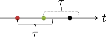
From a physical point of view, the nature of the dead time is determined by the component creating it. Typically, dead time due to the electronic components of the acquisition system is considered to be non-paralyzing, whereas dead time created by the physical process in the detector is often paralyzing.

Modeling the dead time effect on a reactor monitoring system, either operational or experimental, is a very hard theoretical challenge for two main reasons: first, the different dead time models are often too complex to be incorporated in the current mathematical models. Second, the actual dead time effect depends not only on the average count rate but also on time correlations. Therefore, a full theoretical treatment of the dead time effect must be achieved by enforcing the different dead time models on stochastic models of neutron flux. Although in recent years there have been several attempts to account for dead time effects in stochastic models, mainly in the context of neutron multiplicity counting (e.g. [5,6,20]), it is safe to state that the effect of detector dead time on the count histogram is far from being fully understood.

2.2. Reactor noise and the Feynman-α method

Reactor experiments based on sampling higher moments of the neutron count distribution or time correlations between neutrons are often referred to as reactor noise experiments [21]. Noticeable between the different noise techniques is the so-called Feynman-α method, where the variance-to-mean ratio of the number of detections in random (or consecutive) time windows is fitted with the so-called Feynman-Y function.

The Feynman-α method for determining the reactivity of a sub-critical assembly requires sampling the variance and the mean of the number of detections in consecutive (or random) time windows of duration T (T is referred to as the ‘gate’ or ‘gate width’), for varying values of T, and then fitting the sampled values (as a function of T) with the so-called Feynman-Y function.

Sampling the values the Feynman-Y function is typically done in the following manner: for a measurement of duration T_tot, choose N sub-intervals of duration T (T ≪ T_tot) and define the random variable X_i as the number of detections in the ith gate (1 ≤ i ≤ N) and define (1) $$\begin{array}{ccc}\hfill E\left(T\right)& =& \frac{1}{N}\sum _{i=1}^N{X}_i,\hfill \\ \hfill V\left(T\right)& =& \frac{1}{N-1}\sum _{i=1}^N{\left[X_i-E\left(T\right)\right]}^2,\hfill \\ \hfill Y\left(T\right)& =& \frac{V\left(T\right)}{E\left(T\right)}-1.\hfill \end{array}$$(1) In its most primal form (single energy group, no delayed neutrons point-wise model), the Feynman-Y function is given by (2) $$\begin{array}{c}\hfill Y\left(T\right)=Y_{\infty }\times \left(1-\frac{1-e^{-\alpha T}}{\alpha T}\right),\end{array}$$(2) where α is the Rossi-α decay coefficient (assumed positive according to Equation (2(2) $$\begin{array}{c}\hfill Y\left(T\right)=Y_{\infty }\times \left(1-\frac{1-e^{-\alpha T}}{\alpha T}\right),\end{array}$$(2) )) and is defined by α ≡ −ρ_p/Λ, Λ is the prompt neutron generation time, and ρ_p is the prompt reactivity (ρ_p = ρ − β_eff).

Of course, Equation (2(2) $$\begin{array}{c}\hfill Y\left(T\right)=Y_{\infty }\times \left(1-\frac{1-e^{-\alpha T}}{\alpha T}\right),\end{array}$$(2) ) neglects all dead time effects on the neutron count. Since the effect of the dead time is stronger on the second moment of the count distribution, the dead time losses are easily detected by negative values of Y(T) as T approaches zero (rather than a monotonic trend Y(T → 0) → 0) [22]. The most common correction to the Feynman-Y curve due to dead time effect is due to Müller [1], which is achieved by ‘lifting’ the Feynman-Y curve with a factor 2Rτ, where τ is the estimated dead time and R is the estimated count rate. More recent treatment to dead time effect may be found in [13,14,22].

The purpose of the present study is to propose a new method for dead time correction on the Feynman-Y curve.

2.3. Dead time correction using the BEX method

The BEX method for dead time corrections was originally introduced in the context of neutron multiplicity counting [23] and was adopted and examined for reactor monitoring in [15]. The idea behind the BEX method is very simple: consider a detection signal (3) $$\begin{array}{c}\hfill D_T=(t_1,t_2,\dots ,t_i,\cdots ,t_n),t_i<t_{i+1},\end{array}$$(3) describing the detection times in a nuclear system during an interval of duration T. D_T is, in fact, a single realization of a random process, which depends on many parameters characterizing the nuclear system, among them is the dead time of the system, which is denoted by τ₀. Since the present study focuses on the dead time, the random process is denoted by X(T, τ₀).

The measured CPS, given by $\frac{n}{T}$, is a sampling of the average count rate in the random process X(T, τ). The average count rate (including the losses due to a dead time τ) has some functional form f(τ), which depends, of course, on the average CPS. Using this simple terminology, performing a dead time correction on the CPS is nothing more than evaluating f(0) (and the dead time losses is nothing more than f(0) − f(τ)). Of course, sampling f(0) is impossible. On the other hand, for every τ > τ₀, sampling f(τ) can be achieved by artificially ‘enforcing’ a dead time τ on the detection signal D_T, simply by ‘removing’ detections which are in proximity with the previous detection.

This procedure produces a sampling of f(τ) for selected values of τ > τ₀. Then, a curve is fitted to the sampled values of f(τ), and the resulting curve is extrapolated back to zero, to obtain an approximation of f(0) (see [15] for a more detailed description).

The BEX method was tested on a set of seven measurements taken at the MINERVE zero power reactor, in seven different power levels, where the dead time losses ranged between a mere 1.5% and 30%. The method proved very accurate in correcting the CPS within a 1% error bar from the expected value.

In the present study, a generalization of the BEX method is described and implemented to perform dead time corrections to the Feynman-Y curve.

3. Implementation of the BEX method on the Feynman-Y curve

In this section, which is in many ways the main contribution of this study, the method is described in full detail. But before doing so, a short remark is in place; the procedure of imposing a dead time on a detector signal is a very simple one, and one can impose any dead time model she/he chooses, paralyzing or non-paralyzing. On the other hand, imposing a non-paralyzing dead time is bound to create a biasing due to the need to ‘revive’ detections that were never detected (see [15]). For this reason, in the present study, it is assumed that the dead time in the system is a paralyzing one. From a practical point of view, this is a very weak restriction, since, in most modern acquisition systems, the dominant dead time is indeed paralyzing. The data used for demonstration in this section is taken from detector 1 in EXP1 as described in Section 4.1

As before, consider a detection signal (4) $$\begin{array}{c}\hfill D_{T_{tot}}=(t_1,t_2,\dots ,t_i,\cdots ,t_n),t_i<t_{i+1},\end{array}$$(4) describing the detection times in a nuclear system during an interval of duration T_tot. One basic method for sampling the Feynman-Y curve for a given gate T is to divide the signal $D_{T_{tot}}$ in to N consecutive gates of duration T (with N = T_tot/T), define C_n as the number of detections in the nth gate, and then the sampled mean and variance are given by (5) $$\begin{array}{ccc}\hfill E_S\left(T\right)& =& \frac{1}{N}\sum _{n=1}^N{C}_n,\hfill \\ \hfill V_S\left(T\right)& =& \frac{1}{N-1}\sum _{n=1}^N{\left[C_n-E_S\left(T\right)\right]}^2,\hfill \\ \hfill Y_S\left(T\right)& =& \frac{V_S\left(T\right)}{E_S\left(T\right)}-1.\hfill \end{array}$$(5) The series C_n is a realization of another random variable denoted by C(T, τ) due to its dependence, among others, on the dead time. Hence, the sampled value of Y_S(T) is a sampling of a theoretical algebraic combination of the first two moments of C(T, τ), or more precisely, a sampling of (6) $$\begin{array}{c}\hfill Y(T,\tau )=\frac{E\left[C{(T,\tau )}^2\right]-E{\left[C(T,\tau )\right]}^2}{E\left[C(T,\tau )\right]}-1.\end{array}$$(6)

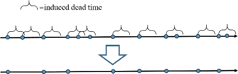
The first thing to observe is that for every τ > τ₀, Y(T, τ) can be sampled from $D_{T_{tot}}$ simply by removing all detections t_j such that t_j − t_{j − 1} < τ (see Figure 2), and then re-calculating the moments as described in Equation (5(5) $$\begin{array}{ccc}\hfill E_S\left(T\right)& =& \frac{1}{N}\sum _{n=1}^N{C}_n,\hfill \\ \hfill V_S\left(T\right)& =& \frac{1}{N-1}\sum _{n=1}^N{\left[C_n-E_S\left(T\right)\right]}^2,\hfill \\ \hfill Y_S\left(T\right)& =& \frac{V_S\left(T\right)}{E_S\left(T\right)}-1.\hfill \end{array}$$(5) ). Clearly, if τ < τ₀, then this procedure will be totally useless, since no detections will be removed. On the other hand, if the procedure is repeated for a range of values of τ, a sampling of Y(T, τ) in that range can be obtained.

Figure 2. Inducing a paralyzing dead time on the detection signal. Each dot represents a detection. If the duration between two consecutive detections is less than the dead time, the later of the two is removed.

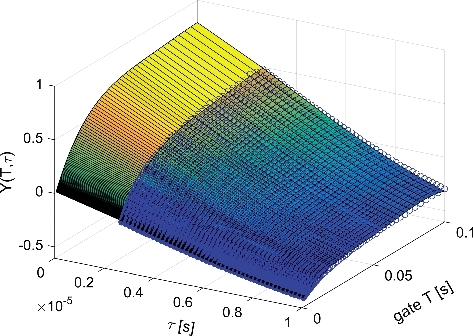
Next, under the very natural assumption that Y(T, τ) is an analytic function of τ, we can estimate the values of Y(T, 0) by fitting a 2-D surface on the sampled data of Y(T, τ), and extrapolate back to τ = 0. To demonstrate the implementation of the BEX method on the Feynman-Y curve, the reader is first referred to Figure 3.

Figure 3. A three-dimensional plot of the BEX surface Y(T, τ). The black dots indicate the τ₀ cut-off, after which the induced dead time changes the values of the variance-to-mean ratio.

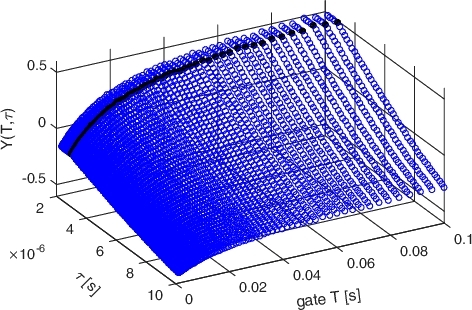
The figure is an implementation of the BEX method (as described above) on a measurement with dead time τ₀ ≈ 3 µs, showing Y(T, τ) as a function of the gate width T and the artificially induced dead time τ. As can be observed, for τ ≤ τ₀, the Feynman-Y curve does not change until the threshold value τ = τ₀ is met (indicated in Figure 3 with black solid dots). However, once the threshold is passed, a monotonic decrease in the Feynman-Y values can be seen. Then, taking only the values computed for τ ≥ τ₀, the data is fitted to a general scheme, and then extrapolated back to zero. Figure 4 represents the implementation of the BEX method to a single ‘slice’: a curve is fitted on the values of Y(T, τ) for a fixed value of T and τ ≥ τ₀. Then, the fitted curve is extrapolated back to zero, and the bisection of the fitted curve and the Y-axis is the corrected value of the Feynman-Y curve. The fit on the entire Y(T, τ) surface (rather than a single value of T) is shown in Figure 5.

Figure 4. Graphic illustration of the BEX method on a single ‘slice’ of the Feynman-Y curve. The fitted curve is second-degree one-dimensional polynomial, i.e. p₀ + p₁τ + p₂τ².

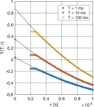
Figure 5. Graphic illustration of the BEX method on the entire Y(T, τ) surface (rather than a single value of T). The fitted surface is a fourth-degree two-dimensional polynomial, i.e. p₀₀ + p₁₀τ + p₀₁T + p₂₀τ² + p₁₁τT + p₀₂T² + p₃₀τ³ + p₂₁τ²T + p₁₂τT² + p₀₃T³ + p₄₀τ⁴ + p₃₁τ³T + p₂₂τ²T² + p₁₃τT³ + p₀₄T⁴.

As in previous implementation of the BEX method, once the fit process is complete, the corrected value of the Feynman-Y curve is obtained by extrapolating back to zero, or simply taking Y(.T|τ = 0). Graphically, the corrected Feynman-Y curve is obtained by the bisection of Y(T, τ) and the T–Y plane.

4. Experimental validation

The aim of the present section is to demonstrate a full implementation of the BEX method on an actual detection signal recorded at the MINERVE zero power reactor (ZPR) and evaluate the performance of the method. To evaluate the performance of the method, the original data recorded from the ZPR suffered a negligible dead time (less than 100 ns) and was only used (in its entirety) as a reference value, while the actual implementation of the method was done on manipulated data, on which a paralyzing dead time was inflicted.

4.1. Experimental setup

The MINERVE reactor is a pool-type (∼120 m³) reactor operating at a maximum power of 100 W with a corresponding thermal flux of 10⁹ n/cm² s [16]. The core is composed of a driver zone, which includes 40 standard highly enriched MTR-type metallic uranium alloy plate assemblies surrounded by a graphite reflector. An experimental zone, in which various UO₂ or MOX cladded fuel pins can be loaded in different lattices, reproducing various neutron spectra [16,24], is located in the center of the driver zone. During the experimental campaign, the central experimental zone was loaded with 770 UO₂ fuel rods arranged in a regular lattice, with a pitch of 1.26 cm, representative of a PWR spectrum. The ²³⁵U enrichment of the uranium is 3%. A schematic drawing of the reactor geometrical configuration during the September 2014 experiments is shown in Figure 6.

Figure 6. Schematic layout of the MINERVE zero power reactor during the noise measurements campaign in September 2014.

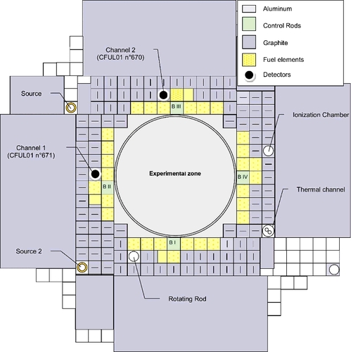
During the measurement campaign, neutron noise experiments were conducted in three reactor states; one very close to critical state (not analyzed in this study) and two different subcritical states marked as ‘EXP1’ and ‘EXP2’, with core negative reactivity of −230 and −120 pcm, respectively, measured by pre-calibrated rod-drop experiment [19]. The different criticality states were obtained by inserting one of the four control rods into the core. The reactor configuration was that of the MAESTRO program [17] (see Figure 6).

Two large fission chambers with approximately 1 g of ²³⁵U (CFUL-01, from PHOTONIS [25]) have been installed next to the driver zone and are denoted n° 670 (near control rod B III) and n° 671 (near control rod B II) in Figure 6. The fission chambers have a high efficiency (1 cps/nv) and a small deadtime (100 ns) when used in pulse mode. Each measurement was recorded by both detectors, resulting in four detection signals to be analyzed. In order to minimize flux disturbances in the detectors during measurement, reactor criticality was controlled by control rod B1, which is far from the two detectors. During the measurements, the power was regulated by an automatic piloting system that makes use of a low-efficiency rotating control rod with cadmium sectors.

The signals were acquired using fast amplifiers (Canberra ADS 7820) and CEA-developed multipurpose acquisition system X-MODE [26]. The signals were acquired in time-stamping mode with a resolution of 25 ns. Measurements EXP1 and EXP2 have been conducted at zero power with count rates around 40 and 77 kcps, respectively. With detector dead time of less than 100 ns, dead time losses and channel shifting errors are negligible. Each of the measurements lasted approximately 5500 seconds. More details on the experimental setup and acquisition systems can be found in [25,27].

For each of the original signals, the Feynman-Y curve is sampled in the interval 10⁻³ ≤ T ≤ 10⁻¹ s, to serve as a reference value. Then, the original data is used to create 12 different signals. From each of the original four signals, three new signals were created by inflicting three different values of paralyzing dead time. A summary of all 12 signals is shown in Table 1.

Table 1. Detector signals with inflicted dead time τ

Signal no.	Experiment	Detector	τ (µs)	CPS reduction
1	EXP1	1	1.37	5%
2			2.2	8%
3			2.7	10%
4		2	1.34	5%
5			2.15	8%
6			2.67	10%
7	EXP2	1	0.77	5%
8			1.2	8%
9			1.5	10%
10		2	0.72	5%
11			1.1	8%
12			1.4	10%

The BEX procedure is implemented on each of the 12 signals and the results are compared with the corresponding reference signal. For the fitting scheme, a second degree polynomial is used for each value of T. In other words, a surface fit is not used, but rather a one-dimensional fit for each ‘slice’ of the function Y(T, τ) (with fixed T).

4.2. Experimental results

The results of the implementation for all 12 signals is shown in Figures 7–10.

Figure 7. Results of the BEX method for all signals created from the first detector in EXP1.

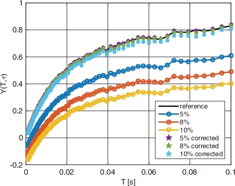
Figure 8. Results of the BEX method for all signals created from the second detector in EXP1.

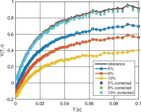
Figure 9. Results of the BEX method for all signals created from the first detector in EXP2.

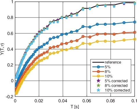
Figure 10. Results of the BEX method for all signals created from the second detector in EXP2.

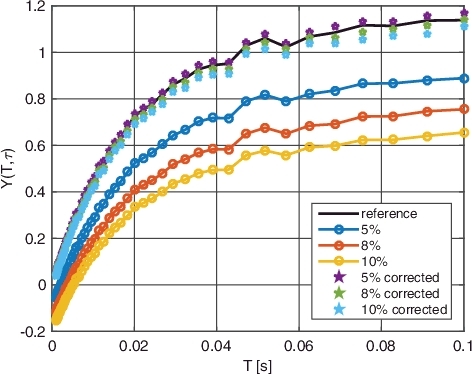
The first thing to notice is that for all 12 examples, the method has successfully ‘lifted’ the Feynman-Y curve towards the reference Feynman-Y curve (created by the original data). Notice that, as expected, the Feynman-Y curve of the manipulated data, before the correction, always obtains negative values as T approaches zero. In corrected curves, the values are ‘lifted’ and negative values no longer appear.

One possible quantification of the ‘goodness’ of the result is the average deviation of the fitted curve Y(T_k|τ → 0) from the reference curve Y(T), which we can define by (7) $$\begin{array}{c}\hfill e_Y[\%]=\frac{1}{N}\sum _{k=1}^N\left|\frac{Y\left(T_k\right)-Y\left(T_k\right|\tau \to 0)}{Y\left(T_k\right)}\right|.\end{array}$$(7) Results are given in Table 2 for different induced dead times, i.e. 5%, 8%, and 10% CPS reduction (see Table 1).

Table 2. Quantification of the goodness of the corrected curves (see Equation (7(7) $$\begin{array}{c}\hfill e_Y[\%]=\frac{1}{N}\sum _{k=1}^N\left|\frac{Y\left(T_k\right)-Y\left(T_k\right|\tau \to 0)}{Y\left(T_k\right)}\right|.\end{array}$$(7) )) for different induced dead times, i.e. 5%, 8%, and 10% CPS reduction (see Table 1)

CPS reduction		5%	8%	10%
EXP1	det. 1	1.5%	4.5%	10.7%
	det. 2	0.9%	2.1%	6.3%
EXP2	det. 1	3.8%	0.7%	3.2%
	det. 2	3.1%	3.8%	7.6%

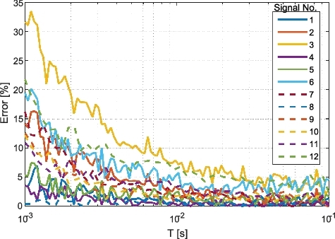
As can be seen, with a single exception, the method performed better for shorter inflicted dead times. However, Table 2 is somewhat misleading, because it does not reveal how the deviation of the Feynman-Y curve affects the reactivity estimation. Moreover, Figure 11 shows the deviation (in %) for all 12 signals as a function of the time gate T. As can be seen, the deviation clearly reduces as T increases. In particular, the deviation depends on the number and distribution of the time gates.

Figure 11. The deviation (%) of the BEX approximation from the Feynman-Y curve with respect to the control values.

A more reliable quantifier for the performance of the method is the estimated α decay constant and reactivity. For that purpose, the delayed neutron fraction was assumed ${\beta }_{\mathtt{eff}}=720$ pcm and the prompt neutron lifetime was assumed Λ = 93 µs, both with uncertainty of 2% [18,19]. Considering that the statistical uncertainty on α due to the fit process is roughly 2.5%, the overall propagated uncertainty on the reactivity, which is given by $\Delta \rho =\sqrt{{\left(\Delta \beta \right)}^2+{\left(\alpha \Delta \Lambda \right)}^2+{\left(\Lambda \Delta \alpha \right)}^2}$, is approximately ±30 pcm. Table 3 gives the reactivity and estimated decay constant for all 12 experiments.

Table 3. The evaluated decay constant and reactivity using the BEX dead time correction method. The propagated uncertainty on the reactivity is approximately ±30 pcm

	α (s^-1)		ρ (pcm)
Signal no.	Estimated	Reference	Estimated	Reference
1	99.8	100.9	−208	−220
2	100.0	100.9	−210	−220
3	100.4	100.9	−214	−220
4	99.4	98.6	−204	−197
5	98.1	98.6	−192	−197
6	97.3	98.6	−185	−197
7	93.8	90.7	−152	−123
8	92.2	90.7	−137	−123
9	89.5	90.7	−112	−123
10	93.1	93.1	−146	−145
11	89.8	93.1	−115	−145
12	88.9	93.1	−107	−145

The results in Table 3 indicate that the method performs very well. The average difference between the reference reactivity and the estimated reactivity (calculated using the BEX method) is 15 pcm, with a maximal deviation of about 40 pcm. Since the statistical uncertainty on the reactivity is estimated at 30 pcm, it is safe to state that the method is successful.

5. Conclusions

A new method for performing dead time corrections on the Feynman-Y variance-to-mean ratio is introduced. The method is based on the simple idea of imposing artificial dead time (of increasing durations) to construct the functional dependence of the Feynman-Y curve on the dead time and then extrapolate the function back to zero. This approach was previously used to perform dead time corrections on the count rate, and the present study is a natural extension to dead time correction of higher moments of the count distribution.

The method was implemented on a set of 12 signals, all created from four in-pile noise experiments signal by imposing artificial dead time.

The performances and accuracy of the method are tested with respect to two scales: deviation from the reference Feynman-Y curve, and deviation from the reference reactivity and decay constant α. Results indicate good performances and accuracy in both aspects, with an average difference between the reference and the BEX-estimated α's of 1.6% and an average difference between the reference and the BEX-estimated reactivity of 15 pcm. Since the overall propagated statistical uncertainty on the reactivity is about 30 pcm, it is safe to state that for all practical purposes, the method can successfully reconstruct the Feynman-Y curve adequately corrected for dead time.

Acknowledgments

Yael Neumeier was partially supported by the Israel Ministry of Energy [contracts number 216-11-008 and 214-11-011] and the PAZY Foundation [contract number 5100012024].

Disclosure statement

No potential conflict of interest was reported by the authors.

Additional information

Funding

Yael Neumeier was partially supported by the Israel Ministry of Energy [contracts number 216-11-008 and 214-11-011] and the PAZY Foundation [contract number 5100012024].

References

- Müller JW. Dead-time problems. Nucl Instrum Methods Phys Res A. 1973;112(1):47–57.
- Müller JW. Generalized dead times. Nucl Instrum Methods Phys Res A. 1991;301(3):543–551.
- Pacilio N. Bernoulli trials and counting correlations in nuclear particles detection. Nucl Instrum Methods Phys Res A. 1966;42(2):241–244.
- Hage W, Cifarelli DM. Correlation analysis with neutron count distribution for a paralyzing dead-time counter for the assay of spontaneous fissioning material. Nucl Sci Eng. 1992;112(2):136–158.
- Pál L, Pázsit I. On some problems in the counting statistics of nuclear particles: investigation of the dead time problems. Nucl Instrum Methods Phys Res A. 2012;693:26–50.
- Dubi C, Israelashvili I, Ridnik T. Analytic model for dead time effect in neutron multiplicity counting. Nucl Sci Eng. 2014;176(3):350–359.
- Carloni F, Corberi A, Marseguerra M, et al. Different methods of dead-time correction in nuclear particles counting distribution. Nucl Instrum Methods Phys Res A. 1969;75(1):155–158.
- Michotte C, Nonis M. Experimental comparison of different dead-time correction techniques in single-channel counting experiments. Nucl Instrum Methods Phys Res A. 2009;608(1):163–168.
- Knoll GF. Radiation detection and measurement. 3rd ed. Orlando (FL): Wiley; 2000.
- Yamane Y, Ito DI. Feynman-α formula with dead time effect for a symmetric coupled-core system. Ann Nucl Energy. 1996;23(12):981–987.
- Yamane Y, Misawa T, Shiroya S, et al. Formulation of data synthesis technique for Feynman-α method. Ann Nucl Energy. 1998;25(1):141–148.
- Degweker SB. Some variants of the Feynman-α method in critical and accelerator driven sub critical systems. Ann Nucl Energy. 2000;27(14):1245–1257.
- Hazama T. Practical correction of dead time effect in variance-to-mean ratio measurement. Ann Nucl Energy. 2003;30(5):615–631.
- Kitamura Y, Fukushima M. Correction of count-loss effect in neutron correlation methods that employ single neutron counting system for subcriticality measurement. J Nucl Sci Technol. 2014;51(6):766–782.
- Gilad E, Dubi C, Geslot B, et al. Dead time corrections using the backward extrapolation method. Nucl Instrum Methods Phys Res A. 2017;854:53–60.
- Bignan G, Fougeras P, Blaise P, et al. Reactor physics experiments on Zero Power Reactors. In: Cacuci DG, editor. Handbook of nuclear engineering. Vol. III. New York, NY: Springer; 2010. p. 2084–2096.
- Leconte P, Geslot B, Gruel A et al, . MAESTRO: an ambitious experimental programme for the improvement of nuclear data of structural, detection, moderating and absorbing materials - first results for nat V, 55Mn, 59Co and 103Rh. In: 3rd ANIMMA, 23–27 June 2013, Marseille, France; 2013. Piscataway, USA: IEEE. p. 282–290.
- Gilad E, Rivin O, Ettedgui H, et al. Experimental estimation of the delayed neutron fraction βeff of the MAESTRO core in the MINERVE zero power reactor. J Nucl Sci Technol. 2015;52(7–8):1026–1033.
- Gilad E, Geslot B, Blaise P, et al. Sensitivity of power spectral density techniques to numerical parameters in analyzing neutron noise experiments. Prog Nucl Energy. 2017. doi:https://doi.org/10.1016/j.pnucene.2017.03.019.
- Hauck DK, Croft S, Evans LG, et al. Study of a theoretical model for the measured gate moments resulting from correlated detection events and an extending dead time. Nucl Instrum Methods Phys Res A. 2013;719:57–69.
- Uhrig RE. Random noise techniques in nuclear reactor systems. New York (NY): Ronald Press Company; 1970.
- Hashimoto K, Ohya K, Yamane Y. Experimental investigations of dead-time effect on Feynman-α method. Ann Nucl Energy. 1996;23(14):1099–1104.
- Ridnik T, Dubi C, Israelashvili I, et al. LIST-mode applications for neutron multiplicity counting. Nucl Instrum Methods Phys Res A. 2014;735:53–59.
- Hudelot JP, Klann R, Fougeras P et al, . OSMOSE: an experimental program for the qualification of integral cross sections of actinides. PHYSOR 2004; 2004 April 25–29; Chicago, IL.
- Geslot B, Gruel A, Pepino A et al, . Pile noise experiment in MINERVE reactor to estimate kinetic parameters using various data processing methods. 4th ANIMMA; 2015 April 20–24; Lisbon.
- Geslot B, Jammes C, Nolibe G et al, . Multimode acquisition system dedicated to experimental neutronic physics. In: 2005 IEEE instrumentation and measurement technology conference proceedings. Vol. 2; 2005. Piscataway, USA: IEEE. p. 1465–1470.
- Perret G. Delayed neutron fraction and prompt decay constant measurement in the MINERVE reactor using the PSI instrumentation. In: 4th ANIMMA, 2015 April, Lisbon. 2015. Piscataway, USA: IEEE. p. 20–24.