The role of the eigenvalue separation in reactor dynamics and neutron noise theory

ABSTRACT

The concept of eigenvalue separation (ES) was introduced in the past for the characterisation of the space-time kinetics of reactor transients, and the stability properties of large loosely coupled cores. However, most of the investigations reported so far concern the determination of the ES itself either from static calculations, or from measurements of the flux tilt or neutron noise cross-correlations. Conclusions on system behaviour were only drawn from the properties of the static eigenfunctions, comparing non-perturbed and perturbed systems, without explicitly solving the time- or frequency-dependent problem. In this paper, we explore the role of the ES on the neutronic response of a critical core to small stochastic perturbations (neutron noise); in particular, the spatial and frequency characteristics of the arising neutron noise as a function of the ES, as well as the spatial structure of the perturbation. It is shown that for systems with small ES and non-uniform perturbations, point kinetics will not dominate even for very low frequencies. The results lend some further insight into the origin and properties of the various types of boiling water reactor instabilities.

KEYWORDS:

• Eigenvalue separation
• neutron noise
• point kinetics
• space dependence
• BWR instability

1. Introduction

The space-time properties of the response of reactor cores to various types of perturbations have been studied extensively in the past. One of these methods is based on the concept of ‘eigenvalue separation’, introduced by Stacey  [1] to characterise the space-time behaviour of reactor cores under transients, including space-dependent xenon oscillations. The expression is commonly abbreviated in text as ES, in some cases as EVS, and its quantitative value in expressions as (E.S.) or (E.S.)_n.

The ES between the static eigenfunctions φ_n and φ₀, n > 0 is defined as (1) $$\begin{array}{c}\hfill {(\text{E.S}.)}_n=\frac{1}{k_n}-\frac{1}{k_0}\ge 0\end{array}$$(1) where k_n and k₀ are the corresponding eigenvalues, k₀ being the effective multiplication factor. The case n = 1 has a special significance, hence it is often used without an index, and in many cases the term‘eigenvalue separation’ is used for this quantity: (2) $$\begin{array}{c}\hfill (\text{E.S}.)\equiv {(\text{E.S}.)}_1=\frac{1}{k_1}-\frac{1}{k_0}\ge 0.\end{array}$$(2) The potential of the concept has been investigated in the past extensively both for describing space-time behaviour under perturbations, the coupling constant of coupled cores, as well as determination of the ES from flux tilt measurements and noise correlation measurements  [2–17]. In particular, at the time of the first visit of one of the authors (I. Pázsit) to Japan in 1990, there was a strong effort at several Japanese universities and research institutes, including the host of the visit, Nagoya University, to study the properties, physical meaning, and the calculation of the ES in loosely coupled systems, as confirmed by the references given in this paper. These investigations confirmed that a small ES increases the proneness of the system to instabilities and enhances the space-dependent behaviour of the system. Systems consisting of loosely coupled regions (such as earlier breeder reactor types with highly enriched regions separated by blankets containing depleted uranium or other fertile material) have a small ES, and hence they show strongly space-dependent kinetic properties.

At the same time, it has to be noted that the objective of these studies was mostly the determination of the ES by numerical or experimental methods, nearly exclusively performed by static methods, or by measurement of the inherent neutron noise in the unperturbed system. A great deal of work was spent on studying the dependence of the magnitude of the ES on static system parameters, including the comparison of non-perturbed and perturbed static systems, without explicitly solving the time- or frequency-dependent problem. In other words, the dependence of the dynamic response of the core for a certain perturbation on the magnitude of the ES has not been a subject of study.

The main objective of this paper is to fill this gap. We shall here investigate the significance of the ES on the dynamic response of a system to small stationary perturbations, leading to what is called power reactor noise. The space-dependent character of the dynamic response of a core to perturbations, in terms of point kinetic or space-dependent behaviour, has traditionally been characterised in terms of system size and the frequency  [18]. These conclusions are drawn directly from the form of the space- and frequency-dependent Green's function of the system, without the need of calculating higher-order eigenfunctions and eigenvalues. Expressing the neutron noise in form of expansion in static eigenfunctions with frequency-dependent coefficients lends the possibility of investigating these properties in terms of the ES, and thus it gives an alternative way of description. This will also illuminate the role of the ES, and will, among others, give alternative insight into already known characteristics, such as the appearance of global and regional oscillations in boiling water reactors (BWRs) from a new angle of view.

As a side-line, it can be mentioned that although the interest in the ES gradually decayed somewhat since the early 2000s, the concept was re-invented in a different context and under a different name. An increasing interest is found in the so-called ‘Dominance Ratio’, often abbreviated as ‘DR’ [19,20], which is the ratio between the fundamental k-eigenvalue to that of the first higher-order eigenvalue k₁. Since there is a one-to-one monotonic relationship between the ES and the dominance ratio, the physical information contained in these two concepts is equivalent. This fact, however, and the knowledge gathered from the investigations of the properties of the ES, seem to have been largely overlooked by the community doing work related to the properties of the dominance ratio.

It has also to be mentioned that the use of the acronym ‘DR’ for the dominance ratio is rather confusing. Namely, another quantity, called the ‘Decay Ratio’, which has been used for the characterising of the stability of the BWRs for many decades, is also commonly abbreviated to ‘DR’  [18,21]. The decay ratio, or the decay constant, is defined as the ratio of the two consecutive peaks of the decaying oscillations of the temporal auto-correlation of the neutron noise at the resonance frequency of the core, usually 0.5 Hz. It has been introduced much earlier than the dominance ratio, and has been used for much longer time  [22–25]. Therefore, in order to avoid misunderstanding, the use of DR for the dominance ratio is strongly discouraged. Not the least since, as it will also be shown in this paper, the concept of the ES, and hence that of the dominance ratio, is useful to explain the appearance of regional oscillations, i.e. a certain type of instability phenomenon, in BWRs. This fact makes it even more justified to keep these two concepts apart, to avoid statements such as ‘a low DR (dominance ratio) leads to a high DR (decay ratio) of the regional mode’.

In this paper, first, it is shown that a general formal solution for the neutron noise in terms of the static eigenfunctions automatically leads to the appearance of the ES in the equations. The characteristics of the neutron noise will then be discussed in terms of the ES and that of the perturbation. After that the relationship between the ES and the coupling strength in a multi-region system will be illustrated in an extreme, in fact pathological, case, which is nevertheless useful to give extended insight. Finally, a quantitative investigation of the dependence of the properties of the neutron noise in a loosely coupled system on the ES will be performed and the results discussed.

2. General principles: neutron noise in terms of the ES

The ES will now be put into the context of neutron noise theory, which concerns the response of the system to small stationary perturbations. One of the basic questions in the theory of neutron noise is the spatial character of the response to a small perturbation, i.e. whether it is point kinetic or space-dependent, and how the system behaves in the limit of low frequencies.

The theory of power reactor noise is described in Ref. [18]; here only a condensed description will be given in one-group diffusion theory in a slab reactor model (one-dimensional (1D) geometry) with one group of delayed neutron precursors. As usual in noise analysis problems, the discussion in the forthcoming refers to systems which are initially critical, i.e. k₀ ≡ k = 1. The corresponding static one-group diffusion equation reads as (3) $$\begin{array}{c}\hfill \Delta {\phi }_0\left(\mathbf{r}\right)+B_0^2{\phi }_0\left(\mathbf{r}\right)=0\end{array}$$(3) with the one-group theory expression of the static buckling as (4) $$\begin{array}{c}\hfill B_0^2=\frac{\nu {\Sigma }_f-{\Sigma }_a}{D}\end{array}$$(4) The system will then be perturbed around the critical state by small stationary fluctuations of the cross sections, which will lead to a time (frequency) dependence of the neutron flux. For simplicity, it will be assumed that only the absorption cross section is fluctuating, i.e. (5) $$\begin{array}{c}\hfill {\Sigma }_a\left(\mathbf{r}\right)\to {\Sigma }_a(\mathbf{r},t)={\Sigma }_a\left(\mathbf{r}\right)+\delta {\Sigma }_a(\mathbf{r},t).\end{array}$$(5) The resulting space- and time-dependent neutron flux will also be split into a mean value (the critical flux) and fluctuations around it, i.e. (6) $$\begin{array}{c}\hfill {\phi }_0\left(\mathbf{r}\right)\to \phi (\mathbf{r},t)={\phi }_0\left(\mathbf{r}\right)+\delta \phi (\mathbf{r},t).\end{array}$$(6) After linearisation, a temporal Fourier transform and elimination of the delayed neutron precursors, the space- and frequency-dependent neutron noise will be given as the solution of the equation  [18] (7) $$\begin{array}{ccc}& & \Delta \delta \phi (\mathbf{r},\omega )+B^2\left(\omega \right)\delta \phi (\mathbf{r},\omega )\hfill \\ & & =S(\mathbf{r},\omega )=\frac{\delta {\Sigma }_a(\mathbf{r},\omega ){\phi }_0\left(\mathbf{r}\right)}{D}\hfill \end{array}$$(7) where the temporal Fourier transform $\delta \phi (\mathbf{r},\omega )$ of $\delta \phi (\mathbf{r},t)$ is defined as (8) $$\begin{array}{c}\hfill \delta \phi (\mathbf{r},\omega )={\int }_{-\infty }^{\infty }{e}^{-i\omega t}\delta \phi (\mathbf{r},t)dt,\end{array}$$(8) and similarly for $\delta {\Sigma }_a(\mathbf{r},\omega )$. The frequency-dependent buckling B²(ω) is given as (9) $$\begin{array}{ccc}\hfill B^2\left(\omega \right)& =& B_0^2\left(1-\frac{\nu {\Sigma }_f}{(\nu {\Sigma }_f-{\Sigma }_a)G_0\left(\omega \right)}\right)\hfill \\ & =& B_0^2-\frac{\nu {\Sigma }_f}{D{G}_0\left(\omega \right)}=B_0^2\left(1-\frac{1}{{\rho }_{\infty }{G}_0\left(\omega \right)}\right)\hfill \end{array}$$(9) with G₀(ω) being the zero power reactor transfer function (10) $$\begin{array}{c}\hfill G_0\left(\omega \right)=\frac{1}{i\omega \left(\Lambda +\frac{\beta }{i\omega +\lambda }\right)};\Lambda =\frac{1}{v\nu {\Sigma }_f}\end{array}$$(10) and (11) $$\begin{array}{c}\hfill {\rho }_{\infty }=1-\frac{1}{k_{\infty }}=\frac{\nu {\Sigma }_f-{\Sigma }_a}{\nu {\Sigma }_f}\end{array}$$(11) being the infinite system reactivity.

The usual discussion on the properties of the system response is based on the solution for the Green's function of Equation (7(7) $$\begin{array}{ccc}& & \Delta \delta \phi (\mathbf{r},\omega )+B^2\left(\omega \right)\delta \phi (\mathbf{r},\omega )\hfill \\ & & =S(\mathbf{r},\omega )=\frac{\delta {\Sigma }_a(\mathbf{r},\omega ){\phi }_0\left(\mathbf{r}\right)}{D}\hfill \end{array}$$(7) ), obeying the equation (12) $$\begin{array}{c}\hfill {\Delta }_{\mathbf{r}}G(\mathbf{r},{\mathbf{r}}^{\text{'}},\omega )+B^2\left(\omega \right)G(\mathbf{r},{\mathbf{r}}^{\text{'}},\omega )=\delta (\mathbf{r}-{\mathbf{r}}^{\text{'}}).\end{array}$$(12) For homogeneous systems, B²(ω) is space-independent, and the Green's function can be given analytically. Its properties can then be analysed in terms of the dependence of B²(ω) on the system size (related to ρ_∞) and the frequency (through G₀(ω)). The analysis readily shows that for perturbations having a non-zero reactivity effect, in the limit of small frequency or small system size, the system behaves in a point kinetic manner, with the amplitude of the response diverging when ω → 0.

The discussion of the same properties in terms of the ES is based on the representation of the space- and frequency-dependent neutron noise in the form of a series expansion by the static spatial eigenfunctions multiplied by frequency-dependent amplitudes. The first term in such a series is the point kinetic component of the noise, whereas the rest represents the space-dependent component. For this, we define the higher-order eigenfunctions as (13) $$\begin{array}{c}\hfill \Delta {\phi }_n\left(\mathbf{r}\right)+B_n^2{\phi }_n\left(\mathbf{r}\right)=0\end{array}$$(13) where now (14) $$\begin{array}{c}\hfill B_n^2=\frac{\frac{\nu {\Sigma }_f}{k_n}-{\Sigma }_a}{D}\end{array}$$(14) Formally, Equation (14(14) $$\begin{array}{c}\hfill B_n^2=\frac{\frac{\nu {\Sigma }_f}{k_n}-{\Sigma }_a}{D}\end{array}$$(14) ) is valid also for the fundamental mode, i.e. for n = 0, with k₀ = 1, since the unperturbed system is critical.

It can be added that expansion of the space-time (space-frequency) dependent flux into other type of complete orthonormal set of spatial eigenfunctions is also possible  [22]. The above choice has the advantage that the equations for the frequency-dependent expansion coefficients will decouple, and the leading term of the expansion is the point kinetic component of the neutron noise.

The solution of Equation (7(7) $$\begin{array}{ccc}& & \Delta \delta \phi (\mathbf{r},\omega )+B^2\left(\omega \right)\delta \phi (\mathbf{r},\omega )\hfill \\ & & =S(\mathbf{r},\omega )=\frac{\delta {\Sigma }_a(\mathbf{r},\omega ){\phi }_0\left(\mathbf{r}\right)}{D}\hfill \end{array}$$(7) ) is now constructed by an expansion into the spatial eigenfunctions ${\phi }_n\left(\mathbf{r}\right)$ with frequency-dependent coefficients: (15) $$\begin{array}{ccc}\hfill \delta \phi (\mathbf{r},\omega )& =& \sum _{n=0}^{\infty }{a}_n\left(\omega \right){\phi }_n\left(\mathbf{r}\right)\hfill \\ & =& a_0\left(\omega \right){\phi }_0\left(\mathbf{r}\right)+\sum _{n=1}^{\infty }{a}_n\left(\omega \right){\phi }_n\left(\mathbf{r}\right)\hfill \end{array}$$(15) Here, the splitting of the sum by separating its first term is only made because it is equal to the point kinetic component of the noise. Similar expansions of the perturbed flux, although for static cases, were considered in connection with the ES in  [2,5,10].

Substituting Equation (15(15) $$\begin{array}{ccc}\hfill \delta \phi (\mathbf{r},\omega )& =& \sum _{n=0}^{\infty }{a}_n\left(\omega \right){\phi }_n\left(\mathbf{r}\right)\hfill \\ & =& a_0\left(\omega \right){\phi }_0\left(\mathbf{r}\right)+\sum _{n=1}^{\infty }{a}_n\left(\omega \right){\phi }_n\left(\mathbf{r}\right)\hfill \end{array}$$(15) ) into Equation (7(7) $$\begin{array}{ccc}& & \Delta \delta \phi (\mathbf{r},\omega )+B^2\left(\omega \right)\delta \phi (\mathbf{r},\omega )\hfill \\ & & =S(\mathbf{r},\omega )=\frac{\delta {\Sigma }_a(\mathbf{r},\omega ){\phi }_0\left(\mathbf{r}\right)}{D}\hfill \end{array}$$(7) ), and using Equation (13(13) $$\begin{array}{c}\hfill \Delta {\phi }_n\left(\mathbf{r}\right)+B_n^2{\phi }_n\left(\mathbf{r}\right)=0\end{array}$$(13) ) for ${\phi }_n\left(\mathbf{r}\right)$ yield (16) $$\begin{array}{ccc}& & \sum _{n=0}^{\infty }{a}_n\left(\omega \right)\left[-B_n^2+B^2\left(\omega \right)\right]{\phi }_n\left(\mathbf{r}\right)=\frac{\delta {\Sigma }_a(\mathbf{r},\omega ){\phi }_0\left(\mathbf{r}\right)}{D}\hfill \end{array}$$(16) Using the definition of the eigenvalue separation (1(1) $$\begin{array}{c}\hfill {(\text{E.S}.)}_n=\frac{1}{k_n}-\frac{1}{k_0}\ge 0\end{array}$$(1) ) and the form of B²(ω) and B²₀ given by Equations (4(4) $$\begin{array}{c}\hfill B_0^2=\frac{\nu {\Sigma }_f-{\Sigma }_a}{D}\end{array}$$(4) ), (9(9) $$\begin{array}{ccc}\hfill B^2\left(\omega \right)& =& B_0^2\left(1-\frac{\nu {\Sigma }_f}{(\nu {\Sigma }_f-{\Sigma }_a)G_0\left(\omega \right)}\right)\hfill \\ & =& B_0^2-\frac{\nu {\Sigma }_f}{D{G}_0\left(\omega \right)}=B_0^2\left(1-\frac{1}{{\rho }_{\infty }{G}_0\left(\omega \right)}\right)\hfill \end{array}$$(9) ), and (14(14) $$\begin{array}{c}\hfill B_n^2=\frac{\frac{\nu {\Sigma }_f}{k_n}-{\Sigma }_a}{D}\end{array}$$(14) ), one finds readily that (17) $$\begin{array}{c}\hfill D\left[-B_n^2+B^2\left(\omega \right)\right]=-\nu {\Sigma }_f\left[{(\text{E.S}.)}_n+G_0^{-1}\left(\omega \right)\right],\end{array}$$(17) where, obviously (E.S.)₀ = 0. Hence, Equation (16(16) $$\begin{array}{ccc}& & \sum _{n=0}^{\infty }{a}_n\left(\omega \right)\left[-B_n^2+B^2\left(\omega \right)\right]{\phi }_n\left(\mathbf{r}\right)=\frac{\delta {\Sigma }_a(\mathbf{r},\omega ){\phi }_0\left(\mathbf{r}\right)}{D}\hfill \end{array}$$(16) ) can be re-written in the form (18) $$\begin{array}{ccc}& & -\sum _{n=0}^{\infty }{a}_n\left(\omega \right)\nu {\Sigma }_f\left[{(\text{E.S}.)}_n+G_0^{-1}\left(\omega \right)\right]{\phi }_n\left(\mathbf{r}\right)\hfill \\ & & =\delta {\Sigma }_a(\mathbf{r},\omega ){\phi }_0\left(\mathbf{r}\right)\hfill \end{array}$$(18) For a homogeneous system, i.e. when B²(ω) is space-independent, the equations for the a_n(ω) for different values of n decouple, due to the orthogonality relations of the static eigenfunctions ${\phi }_n\left(\mathbf{r}\right)$. Hence, multiplying Equation (18(18) $$\begin{array}{ccc}& & -\sum _{n=0}^{\infty }{a}_n\left(\omega \right)\nu {\Sigma }_f\left[{(\text{E.S}.)}_n+G_0^{-1}\left(\omega \right)\right]{\phi }_n\left(\mathbf{r}\right)\hfill \\ & & =\delta {\Sigma }_a(\mathbf{r},\omega ){\phi }_0\left(\mathbf{r}\right)\hfill \end{array}$$(18) ) by ${\phi }_k\left(\mathbf{r}\right)$, integrating over the reactor volume V_R, and also utilising Equations (9(9) $$\begin{array}{ccc}\hfill B^2\left(\omega \right)& =& B_0^2\left(1-\frac{\nu {\Sigma }_f}{(\nu {\Sigma }_f-{\Sigma }_a)G_0\left(\omega \right)}\right)\hfill \\ & =& B_0^2-\frac{\nu {\Sigma }_f}{D{G}_0\left(\omega \right)}=B_0^2\left(1-\frac{1}{{\rho }_{\infty }{G}_0\left(\omega \right)}\right)\hfill \end{array}$$(9) ), (13(13) $$\begin{array}{c}\hfill \Delta {\phi }_n\left(\mathbf{r}\right)+B_n^2{\phi }_n\left(\mathbf{r}\right)=0\end{array}$$(13) ), and (14(14) $$\begin{array}{c}\hfill B_n^2=\frac{\frac{\nu {\Sigma }_f}{k_n}-{\Sigma }_a}{D}\end{array}$$(14) ), one obtains (19) $$\begin{array}{ccc}\hfill a_k\left(\omega \right)& =& -\frac{{\int }_{V_R}\delta {\Sigma }_a(\mathbf{r},\omega ){\phi }_0\left(\mathbf{r}\right){\phi }_k\left(\mathbf{r}\right)d\mathbf{r}}{\nu {\Sigma }_f\left[{(\text{E.S}.)}_n+G_0^{-1}\left(\omega \right)\right]{\int }_{V_R}{\phi }_k^2\left(\mathbf{r}\right)d\mathbf{r}};\hfill \\ \hfill k& =& 0,1,2\cdots \hfill \end{array}$$(19) Using this in Equation (15(15) $$\begin{array}{ccc}\hfill \delta \phi (\mathbf{r},\omega )& =& \sum _{n=0}^{\infty }{a}_n\left(\omega \right){\phi }_n\left(\mathbf{r}\right)\hfill \\ & =& a_0\left(\omega \right){\phi }_0\left(\mathbf{r}\right)+\sum _{n=1}^{\infty }{a}_n\left(\omega \right){\phi }_n\left(\mathbf{r}\right)\hfill \end{array}$$(15) ) and also by recalling the perturbation formula of calculating the reactivity in first order of the perturbation yields (20) $$\begin{array}{ccc}\hfill \delta \phi (\mathbf{r},\omega )& =& \rho \left(\omega \right)G_0\left(\omega \right){\phi }_0\left(\mathbf{r}\right)\hfill \\ & & +\sum _{n=1}^{\infty }\frac{\delta {\rho }_n\left(\omega \right)}{\left[{(\text{E.S}.)}_n+G_0^{-1}\left(\omega \right)\right]}{\phi }_n\left(\mathbf{r}\right)\hfill \end{array}$$(20)

Here, the definition (21) $$\begin{array}{ccc}\hfill \delta {\rho }_n\left(\omega \right)& =& \frac{-{\int }_{V_R}\delta {\Sigma }_a(\mathbf{r},\omega ){\phi }_0\left(\mathbf{r}\right){\phi }_n\left(\mathbf{r}\right)d\mathbf{r}}{\nu {\Sigma }_f{\int }_{V_R}{\phi }_n^2\left(\mathbf{r}\right)d\mathbf{r}};\hfill \\ \hfill n& =& 0,1,2,\cdots \hfill \end{array}$$(21) was introduced. It is to be stressed that δρ_n(ω) has nothing to do with the static higher-order reactivity ρ_n = 1 − 1/k_n, which is a property of the unperturbed system; rather, it stands for the higher-order reactivity effect of the perturbation which excites the nth higher-order mode in the response of the system¹ [2]. It is also a special case of the expression ρ^F_mn of Ref. [22] for m = 0. In other words, δρ_n(ω) can be considered as the generalisation of the conventional perturbation theory formula for the reactivity. In analogy with the conventional reactivity ρ(ω) ≡ δρ₀(ω), which is the projection of the perturbation $S(\mathbf{r},\omega )$ to the fundamental mode ${\phi }_0\left(\mathbf{r}\right)$ and which excites the fundamental mode (i.e. the point kinetic or ‘reactivity’ component of the noise), for n ≥ 1, the term δρ_n(ω) can be interpreted as the projection of the perturbation to the nth higher harmonic, and which thus excites the nth higher-order eigenfunction.

From Equation (20(20) $$\begin{array}{ccc}\hfill \delta \phi (\mathbf{r},\omega )& =& \rho \left(\omega \right)G_0\left(\omega \right){\phi }_0\left(\mathbf{r}\right)\hfill \\ & & +\sum _{n=1}^{\infty }\frac{\delta {\rho }_n\left(\omega \right)}{\left[{(\text{E.S}.)}_n+G_0^{-1}\left(\omega \right)\right]}{\phi }_n\left(\mathbf{r}\right)\hfill \end{array}$$(20) ), an analysis of the induced reactor noise, similar to the one based on the analytic solution for the Green's function mentioned earlier, can be made as follows:

(1)	For ω → 0, G0(ω) → ∞. Since (E.S.)0 = 0, whereas (E.S.)n > 0 for n ≥ 1, if ρ(ω) ≠ 0, the first term will dominate, and point kinetic behaviour will prevail.
(2)	If the perturbation is spatially homogeneous (space-independent), i.e. $\delta {\Sigma }_a(\mathbf{r},\omega )=\delta {\Sigma }_a\left(\omega \right)$, then, due to the orthogonality relationships between φ0 and φn for n > 0 in Equation (21(21) $$\begin{array}{ccc}\hfill \delta {\rho }_n\left(\omega \right)& =& \frac{-{\int }_{V_R}\delta {\Sigma }_a(\mathbf{r},\omega ){\phi }_0\left(\mathbf{r}\right){\phi }_n\left(\mathbf{r}\right)d\mathbf{r}}{\nu {\Sigma }_f{\int }_{V_R}{\phi }_n^2\left(\mathbf{r}\right)d\mathbf{r}};\hfill \\ \hfill n& =& 0,1,2,\cdots \hfill \end{array}$$(21) ), δρn(ω) = 0 and hence an(ω) = 0 for n ≥ 1. Thus, point-reactor behaviour exists for any ω (i.e. even for arbitrarily high frequencies).
(3)	If $\delta {\Sigma }_a(\mathbf{r},\omega )$ is an odd (asymmetric) function of $\mathbf{r}$, or better to say in any case when (22) $$\begin{array}{c}\hfill {\int }_{V_R}\delta {\Sigma }_a(\mathbf{r},\omega ){\phi }_0^2\left(\mathbf{r}\right)d\mathbf{r}=0,\end{array}$$(22) one has ρ(ω) = 0, and hence the reactivity term (point-reactor term) equals zero. That is, in such cases, point-reactor behaviour never exists, not even for very low frequencies.

These remarks will now be complemented with further aspects which are related to the ES. Assume now that in Equation (20(20) $$\begin{array}{ccc}\hfill \delta \phi (\mathbf{r},\omega )& =& \rho \left(\omega \right)G_0\left(\omega \right){\phi }_0\left(\mathbf{r}\right)\hfill \\ & & +\sum _{n=1}^{\infty }\frac{\delta {\rho }_n\left(\omega \right)}{\left[{(\text{E.S}.)}_n+G_0^{-1}\left(\omega \right)\right]}{\phi }_n\left(\mathbf{r}\right)\hfill \end{array}$$(20) ), one has (E.S.)₁ ≡ (E.S.) = ϵ < <1, more concretely ϵ < <β, which implies k₁ ≈ k₀. We will also assume that (E.S.)_n > >(E.S.), and for the sake of the argument also that (E.S.)_n > β for n ≥ 2. Then, separating out the first term of the sum in Equation (20(20) $$\begin{array}{ccc}\hfill \delta \phi (\mathbf{r},\omega )& =& \rho \left(\omega \right)G_0\left(\omega \right){\phi }_0\left(\mathbf{r}\right)\hfill \\ & & +\sum _{n=1}^{\infty }\frac{\delta {\rho }_n\left(\omega \right)}{\left[{(\text{E.S}.)}_n+G_0^{-1}\left(\omega \right)\right]}{\phi }_n\left(\mathbf{r}\right)\hfill \end{array}$$(20) ), one can write (23) $$\begin{array}{ccc}\hfill \delta \phi (\mathbf{r},\omega )& =& \rho \left(\omega \right)G_0\left(\omega \right){\phi }_0\left(\mathbf{r}\right)+\frac{\delta {\rho }_1\left(\omega \right)}{\epsilon +G_0^{-1}\left(\omega \right)}{\phi }_1\left(\mathbf{r}\right)\hfill \\ & & +\sum _{n=2}^{\infty }\frac{\delta {\rho }_n\left(\omega \right)}{\left[{(E.S.)}_n+G_0^{-1}\left(\omega \right)\right]}{\phi }_n\left(\mathbf{r}\right)\hfill \end{array}$$(23)

Since at the plateau frequencies λ ≤ ω ≤ β/Λ the amplitude of the zero power transfer function is |G₀(ω)| ≈ 1/β, with the earlier assumptions (and provided that all the ρ_n are larger than zero and of comparable order of amplitude), at the plateau frequencies, on the right hand side (r.h.s.) of Equation (23(23) $$\begin{array}{ccc}\hfill \delta \phi (\mathbf{r},\omega )& =& \rho \left(\omega \right)G_0\left(\omega \right){\phi }_0\left(\mathbf{r}\right)+\frac{\delta {\rho }_1\left(\omega \right)}{\epsilon +G_0^{-1}\left(\omega \right)}{\phi }_1\left(\mathbf{r}\right)\hfill \\ & & +\sum _{n=2}^{\infty }\frac{\delta {\rho }_n\left(\omega \right)}{\left[{(E.S.)}_n+G_0^{-1}\left(\omega \right)\right]}{\phi }_n\left(\mathbf{r}\right)\hfill \end{array}$$(23) ) the first two terms dominate over the rest. Thus, for plateau frequencies one can write (24) $$\begin{array}{c}\hfill \delta \phi (\mathbf{r},\omega )\approx \rho \left(\omega \right)G_0\left(\omega \right){\phi }_0\left(\mathbf{r}\right)+\delta {\rho }_1\left(\omega \right)G_0\left(\omega \right){\phi }_1\left(\mathbf{r}\right)\end{array}$$(24) This form is of course only valid at plateau frequencies and below, but only until |G₀(ω)| < 1/ϵ. For any given value of (E.S.) = ϵ, in the limit ω → 0, if ω is sufficiently small, eventually the first term (the point kinetic term) on the r.h.s. of Equation (23(23) $$\begin{array}{ccc}\hfill \delta \phi (\mathbf{r},\omega )& =& \rho \left(\omega \right)G_0\left(\omega \right){\phi }_0\left(\mathbf{r}\right)+\frac{\delta {\rho }_1\left(\omega \right)}{\epsilon +G_0^{-1}\left(\omega \right)}{\phi }_1\left(\mathbf{r}\right)\hfill \\ & & +\sum _{n=2}^{\infty }\frac{\delta {\rho }_n\left(\omega \right)}{\left[{(E.S.)}_n+G_0^{-1}\left(\omega \right)\right]}{\phi }_n\left(\mathbf{r}\right)\hfill \end{array}$$(23) ) or Equation (24(24) $$\begin{array}{c}\hfill \delta \phi (\mathbf{r},\omega )\approx \rho \left(\omega \right)G_0\left(\omega \right){\phi }_0\left(\mathbf{r}\right)+\delta {\rho }_1\left(\omega \right)G_0\left(\omega \right){\phi }_1\left(\mathbf{r}\right)\end{array}$$(24) ) will dominate. However, if ϵ is sufficiently small, this will happen only at very low frequencies. That is, the form (23(23) $$\begin{array}{ccc}\hfill \delta \phi (\mathbf{r},\omega )& =& \rho \left(\omega \right)G_0\left(\omega \right){\phi }_0\left(\mathbf{r}\right)+\frac{\delta {\rho }_1\left(\omega \right)}{\epsilon +G_0^{-1}\left(\omega \right)}{\phi }_1\left(\mathbf{r}\right)\hfill \\ & & +\sum _{n=2}^{\infty }\frac{\delta {\rho }_n\left(\omega \right)}{\left[{(E.S.)}_n+G_0^{-1}\left(\omega \right)\right]}{\phi }_n\left(\mathbf{r}\right)\hfill \end{array}$$(23) ) will remain valid, with its second term being comparable to the point kinetic term, and if |δρ₁(ω)| > |ρ(ω)|, it will even dominate over it, even for frequencies far below the plateau region. This means that space-dependent behaviour, i.e. deviation from the point kinetic behaviour, will prevail for much lower frequencies than usual.

The above is of course a consequence of the fact that in this case even the first harmonic is ‘close to critical’. A non-zero, but sufficiently small ES means, according to the above analysis, that space-dependent behaviour will be sustained even for low frequencies, way below the plateau frequencies, and also the amplitude of the space-dependent part of the response can be rather high. In the hypothetical case of (E.S.) = 0 (such an extreme case will be discussed in the forthcoming), a perturbation which can excite the first higher-order mode will lead to a diverging amplitude for ω → 0, for exactly the same reasons as for the point kinetic term in the cases when ρ(ω) ≠ 0.

The influence of the ES on the stability of the system can thus be refined in view of the above analysis. Let us define a stable system as one characterised with a small amplitude response to a certain perturbation and an unstable system as one with a large amplitude response to the same perturbation. Then, one can say that systems with a large ES are unstable for perturbations with a reactivity effect at low frequencies, but are stable for perturbations without (or with a very small) reactivity effect. Systems with a very small ES are still unstable for perturbations with a reactivity effect at low frequencies, but they will be also unstable for perturbations without a reactivity effect, as long as δρ₁(ω) ≠ 0. Since, in reality, many perturbations are of local character (moving of an individual control rod, fuel, or control rod vibrations in a pressurized water reactor (PWR), local channel blockage in a BWR, etc.), for these cases it is valid that |δρ₁(ω)| ≈ |ρ(ω)|. For an asymmetric perturbation, for which Equation (22(22) $$\begin{array}{c}\hfill {\int }_{V_R}\delta {\Sigma }_a(\mathbf{r},\omega ){\phi }_0^2\left(\mathbf{r}\right)d\mathbf{r}=0,\end{array}$$(22) ) holds exactly or approximately, one has even |δρ₁(ω)| > >|ρ(ω)|. For such perturbations, a system will become unstable for low frequencies if it has a small ES, despite that there is no reactivity perturbation. This is for instance the case of regional (out-of-phase) BWR oscillations [22–25].

One drawback of the discussion so far, which makes it somewhat trivial, is that the formulae are only valid for homogeneous systems. For homogeneous systems, the only way of achieving a small (E.S.) is to have a large system size. In that case, not only the fundamental (E.S.) but all the higher-order (E.S.)_n will be small, and the separation of the first higher eigenfunction as in Equation (23(23) $$\begin{array}{ccc}\hfill \delta \phi (\mathbf{r},\omega )& =& \rho \left(\omega \right)G_0\left(\omega \right){\phi }_0\left(\mathbf{r}\right)+\frac{\delta {\rho }_1\left(\omega \right)}{\epsilon +G_0^{-1}\left(\omega \right)}{\phi }_1\left(\mathbf{r}\right)\hfill \\ & & +\sum _{n=2}^{\infty }\frac{\delta {\rho }_n\left(\omega \right)}{\left[{(E.S.)}_n+G_0^{-1}\left(\omega \right)\right]}{\phi }_n\left(\mathbf{r}\right)\hfill \end{array}$$(23) ) is not justified. Physically, this means that generally, many modes will be excited simultaneously. A localised perturbation will hence lead to a space-dependent response, in which a large number of higher-order modes coexist (such as in a localised response), and the first harmonic is not favoured over the others in general.

To have a small (E.S.) but much larger (E.S.)_n for n > 1, one needs a loosely coupled core, i.e. an inhomogeneous system. A typical, and for the practical applications, most relevant case is a piecewise homogeneous system, in which high multiplication areas (the fissile regions) are separated by low multiplication regions (breeding blanket regions). For such systems, in which νΣ_f, and hence the prompt neutron generation time 1/(v νΣ_f) are different for the different regions, the corresponding frequency-dependent functions of the respective regions, which are analogous in frequency dependence to the traditional G₀(ω), will also be different for the different regions in Equation (18(18) $$\begin{array}{ccc}& & -\sum _{n=0}^{\infty }{a}_n\left(\omega \right)\nu {\Sigma }_f\left[{(\text{E.S}.)}_n+G_0^{-1}\left(\omega \right)\right]{\phi }_n\left(\mathbf{r}\right)\hfill \\ & & =\delta {\Sigma }_a(\mathbf{r},\omega ){\phi }_0\left(\mathbf{r}\right)\hfill \end{array}$$(18) ) (c.f. Equation (10(10) $$\begin{array}{c}\hfill G_0\left(\omega \right)=\frac{1}{i\omega \left(\Lambda +\frac{\beta }{i\omega +\lambda }\right)};\Lambda =\frac{1}{v\nu {\Sigma }_f}\end{array}$$(10) )).

Because of this, the orthogonality relations separating the equations for the a_n(ω) are not valid any longer. Thus, the equations for the a_i(ω) for different i values will not decouple, and their determination becomes cumbersome. Although, then, the conclusions drawn in the previous derivations related to homogeneous systems on the asymptotic behaviour of the a_i(ω) are not directly transferable to inhomogeneous systems, on physical grounds it can be expected (and our quantitative studies in Section 5 will confirm it) that the solution can still be approximated by the first two terms as (25) $$\begin{array}{c}\hfill \delta \phi (\mathbf{r},\omega )\approx a_0\left(\omega \right){\phi }_0\left(\mathbf{r}\right)+a_1\left(\omega \right){\phi }_1\left(\mathbf{r}\right),\end{array}$$(25) although the quantities a₀ and a₁ will not be simply expressible with the reactivities δρ_n(ω), and the zero power reactor transfer function G₀(ω) of the full system.

On the other hand, in a simple 1D system of two homogeneous coupled cores separated with a homogeneous region of low or no multiplication, analytical solutions can be obtained for the full space-frequency dependent case by constructing closed form analytical solutions in each region, with coefficients that are determined from the interface and boundary conditions. From the full solution, the frequency-dependent coefficients of the various modes can be extracted by projection of the full solution to the respective eigenfunctions, and their frequency dependence investigated quantitatively. Such a case will be considered in Section 5. Before turning to such a realistic case, we will consider an extreme model case with exactly zero ES, because it will give insight into the properties of the ES and its influence on the system behaviour.

3. Illustration in a simple extreme case

In the continuation, we shall discuss a simple, although somewhat extreme example which will serve to illustrate the fact how the ES can be zero, and how in such a coupled core system a space-dependent instability can occur even for a perturbation without a reactivity effect.

The system to be considered is admittedly pathological, because it will consist of two cores completely separated from each other by, e.g. a ‘black’ absorbing material. This means that there is no neutronic coupling between the two cores. Of course, in practice there is no reason why one should treat two independent cores as one system. However, they can be considered as the limiting case of two loosely coupled systems, in which the coupling strength tends to zero, and hence it is an extreme (unrealistic) limit of a realistic case.

We will use a 1D one-group model, the two cores lying symmetrically around the origin with an extrapolated thickness H each, with the extrapolated boundaries of the outer edges of the two cores lying at x = ±a. By having no coupling, both cores can be critical, supercritical, or subcritical individually, and the compound system is critical, supercritical, or subcritical if, asymptotically, the flux is constant at least in one of the systems and not diverging in the other, or diverging at least in one of the cores, or vanishes in both cores, respectively. For simplicity, we chose the same material for both cores, hence they will be critical, subcritical, or supercritical simultaneously, and we will consider the initial system as critical. That means that one has (26) $$\begin{array}{c}\hfill B_0=\frac{\pi }{H}\end{array}$$(26) and k₀ = 1. An important point is that the k_n eigenvalues refer to the aggregate system (for the two cores together as one system), i.e. no different k_n or B²_n values are permitted separately for the two cores. 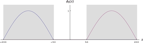The corresponding fundamental mode flux, φ₀(x) is equal to (27) $$\begin{array}{ccc}\hfill {\phi }_0\left(x\right)& =& A_{0}sin\left[B_0(x+a)\right]\hfill \\ & & \text{for}-a<x<-a+H;\hfill \\ \hfill {\phi }_0\left(x\right)& =& A_{0}sin\left[B_0(x-a+H)\right]\hfill \\ & & \text{for}a-H<x<a;\hfill \\ \hfill {\phi }_0\left(x\right)& =& 0\text{otherwise}.\hfill \end{array}$$(27) with A₀ > 0. An illustration for the case a = 200, H = 150, and A₀ = 1 is given in Figure 1.

Figure 1. The fundamental mode φ₀(x) in the system of two decoupled cores.

Actually, the amplitudes in the left and right cores do not necessarily need to be equal; they were here chosen to be equal for convenience. However, if there exists a homogeneous absorbing material between the two cores, the two amplitudes will be equal. So if one treats a decoupled system as a limit of a previously loosely coupled system, the choice of the symmetric amplitudes is plausible.

The interesting aspect comes when we want to determine the first harmonic solution φ₁(x) in this system. We find that a solution which is orthogonal to φ₀(x), and hence is an independent solution, is given as (28) $$\begin{array}{ccc}\hfill {\phi }_1\left(x\right)& =& -A_{1}sin\left[B_0(x+a)\right]\hfill \\ & & \text{for}-a<x<-a+H;\hfill \\ \hfill {\phi }_1\left(x\right)& =& A_{1}sin\left[B_0(x-a+H)\right]\hfill \\ & & \text{for}a-H<x<a;\hfill \\ \hfill {\phi }_1\left(x\right)& =& 0\text{otherwise}.\hfill \end{array}$$(28) This case is illustrated in Figure 2, with A₁ = 1.

Figure 2. The first higher-order eigenfunction φ₁(x) in the system of two decoupled cores.

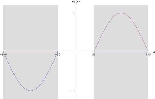
The fact that the buckling appearing in expression (28(28) $$\begin{array}{ccc}\hfill {\phi }_1\left(x\right)& =& -A_{1}sin\left[B_0(x+a)\right]\hfill \\ & & \text{for}-a<x<-a+H;\hfill \\ \hfill {\phi }_1\left(x\right)& =& A_{1}sin\left[B_0(x-a+H)\right]\hfill \\ & & \text{for}a-H<x<a;\hfill \\ \hfill {\phi }_1\left(x\right)& =& 0\text{otherwise}.\hfill \end{array}$$(28) ) is the same as the critical buckling B₀ yields that k₁ = k₀ = 1, and hence one has the case of (E.S.) = 0. It is also easy to confirm that for n > 1, one has (E.S.)_n ≥ 0.

It is now straightforward to interpret how a divergent space-dependent noise arises (or the fact that point kinetic behaviour does not become dominating) in such a pathological system for ω → 0. Assume now a frequency-independent (white noise) localised perturbation of the variable absorber type at the centre of the r.h.s. core²: (29) $$\begin{array}{c}\hfill \delta {\Sigma }_a(x,\omega )=\gamma \delta (x-a+H/2)\end{array}$$(29) The position of the perturbation is indicated with a thick vertical line at x = 125 cm in Figure 3, which shows both the fundamental mode φ₀(x) and the first harmonic φ₁(x) together. In the r.h.s. core, i.e. from x = 50 to x = 200 cm, φ₀(x) completely overlaps with φ₁(x).

Figure 3. The first two lowest order eigenfunctions φ₀(x) and φ₁(x) of the decoupled system, together with the indication of a localised perturbation. In the right hand side core, φ₀(x) and φ₁(x) are identical.

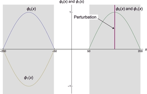
Assume now for simplicity of the reasoning equal amplitudes of the two eigenfunctions, i.e. A₀ = A₁, which corresponds to how the figure is plotted. (It can be shown that the final conclusion of the forthcoming discussion does not depend on the equality of the flux amplitudes.) Then, from the perturbation formula one obtains that ρ(ω) = δρ₁(ω) = const ≡ ρ. Letting now ω → 0, the last term on the r.h.s. of Equation (23(23) $$\begin{array}{ccc}\hfill \delta \phi (\mathbf{r},\omega )& =& \rho \left(\omega \right)G_0\left(\omega \right){\phi }_0\left(\mathbf{r}\right)+\frac{\delta {\rho }_1\left(\omega \right)}{\epsilon +G_0^{-1}\left(\omega \right)}{\phi }_1\left(\mathbf{r}\right)\hfill \\ & & +\sum _{n=2}^{\infty }\frac{\delta {\rho }_n\left(\omega \right)}{\left[{(E.S.)}_n+G_0^{-1}\left(\omega \right)\right]}{\phi }_n\left(\mathbf{r}\right)\hfill \end{array}$$(23) ) can be neglected in comparison to the first and second terms, yielding (30) $$\begin{array}{c}\hfill \delta \phi (x,\omega )\approx \rho G_0\left(\omega \right)[{\phi }_0\left(x\right)+{\phi }_1\left(x\right)]\end{array}$$(30) As it is also seen in Figure 3, the sum of the two eigenfunctions is zero in the left hand side slab, and is equal to 2φ₀(x) in the r.h.s. slab. As is obvious, this behaviour is neither point kinetic, nor fully space-dependent (i.e. without a point kinetic term); it has equal contributions from both the fundamental mode (point kinetic component) and the first higher-order mode (a full space dependent component).

This is of course a somewhat artificial result which considers simultaneously two cores that are not connected. The same result could be obtained in a simpler way, by noting that if only one of two decoupled cores is perturbed, then only that core can have any response, so the fact that there will be no response in the other core, and which we derived in the foregoing as a result of the cancellation of two quantities of opposite sign, will be trivial if we treat the two cores separately. (On the other hand, the fact that we got the correct result, verifiable by other means, shows the correctness of the first harmonic φ₁(x), whose construction might have felt artificial.) If we only consider the perturbed core, then of course the response in that core will be point kinetic at low frequencies. Even quantitatively, we obtain the same result; Equation (30(30) $$\begin{array}{c}\hfill \delta \phi (x,\omega )\approx \rho G_0\left(\omega \right)[{\phi }_0\left(x\right)+{\phi }_1\left(x\right)]\end{array}$$(30) ) will yield for the noise in ‘core II’ (the r.h.s. slab) the result (31) $$\begin{array}{c}\hfill \delta \phi (x,\omega )\approx \rho G_0\left(\omega \right)2sin\left[B_0(x-a+H)\right].\end{array}$$(31) This is the same result as what we obtain by only considering core II. For this case, one will have (32) $$\begin{array}{c}\hfill {\phi }_0\left(x\right)=sin\left[B_0(x-a+H)\right]\end{array}$$(32) and (33) $$\begin{array}{c}\hfill {\phi }_1\left(x\right)=sin\left[2B_0(x-a+H)\right]\end{array}$$(33) That is, B₁ = 2B₀, hence k₁ ≠ k₀ and (E.S.) ≠ 0. Therefore, the second term of Equation (24(23) $$\begin{array}{ccc}\hfill \delta \phi (\mathbf{r},\omega )& =& \rho \left(\omega \right)G_0\left(\omega \right){\phi }_0\left(\mathbf{r}\right)+\frac{\delta {\rho }_1\left(\omega \right)}{\epsilon +G_0^{-1}\left(\omega \right)}{\phi }_1\left(\mathbf{r}\right)\hfill \\ & & +\sum _{n=2}^{\infty }\frac{\delta {\rho }_n\left(\omega \right)}{\left[{(E.S.)}_n+G_0^{-1}\left(\omega \right)\right]}{\phi }_n\left(\mathbf{r}\right)\hfill \end{array}$$(23) ) can be neglected, and Equations (30(30) $$\begin{array}{c}\hfill \delta \phi (x,\omega )\approx \rho G_0\left(\omega \right)[{\phi }_0\left(x\right)+{\phi }_1\left(x\right)]\end{array}$$(30) ) and (31(31) $$\begin{array}{c}\hfill \delta \phi (x,\omega )\approx \rho G_0\left(\omega \right)2sin\left[B_0(x-a+H)\right].\end{array}$$(31) ) will hence take the form (34) $$\begin{array}{c}\hfill \delta \phi (x,\omega )\approx {\rho }_{1\text{core}}{G}_0\left(\omega \right)sin\left[B_0(x-a+H)\right]\end{array}$$(34) where ρ_1core is the reactivity effect of the perturbation if only one core is considered. This is naturally larger than the reactivity effect in the two-core system. One has (35) $$\begin{array}{c}\hfill {\rho }_{1\text{core}}=2\rho \end{array}$$(35) because (36) $$\begin{array}{c}\hfill {\int }_{V_{2\text{cores}}}{\phi }_0^2\left(x\right)dx=2{\int }_{V_{1\text{core}}}{\phi }_0^2\left(x\right)dx\end{array}$$(36) (cf. also Equation (21(21) $$\begin{array}{ccc}\hfill \delta {\rho }_n\left(\omega \right)& =& \frac{-{\int }_{V_R}\delta {\Sigma }_a(\mathbf{r},\omega ){\phi }_0\left(\mathbf{r}\right){\phi }_n\left(\mathbf{r}\right)d\mathbf{r}}{\nu {\Sigma }_f{\int }_{V_R}{\phi }_n^2\left(\mathbf{r}\right)d\mathbf{r}};\hfill \\ \hfill n& =& 0,1,2,\cdots \hfill \end{array}$$(21) )). This shows that we get exactly the same result as when considering a system of two cores simultaneously, which shows that the results obtained from the latter are justified.

One can even go one step further and consider the aggregate effect of two perturbations, by adding another localised perturbation in the middle of core I, i.e. the left hand side one, to the previous one, Equation (29(29) $$\begin{array}{c}\hfill \delta {\Sigma }_a(x,\omega )=\gamma \delta (x-a+H/2)\end{array}$$(29) ) representing an absorber of variable strength, but fluctuating in opposite phase. The absorption cross section fluctuation will then have the form (37) $$\begin{array}{c}\hfill \delta {\Sigma }_a(x,\omega )=-\gamma \delta (x+a-H/2)+\gamma \delta (x-a+H/2)\end{array}$$(37) As it is also easy to see intuitively, the total reactivity effect of this perturbation is zero, i.e. ρ(ω) = 0 whereas δρ₁(ω) ≠ 0. Trivially, δρ₁(ω) will be twice as big as in the previous case, when it was equal to ρ, i.e. it was equal to the reactivity effect of the perturbation when the two cores were considered as one system. So we write (38) $$\begin{array}{c}\hfill \delta {\rho }_1\left(\omega \right)=2\rho \end{array}$$(38) where we shall remember that ρ stands for the reactivity effect of the previous perturbation. In view of the fact that the reactivity in the present case is zero, the noise can be approximated for low frequencies as (39) $$\begin{array}{c}\hfill \delta \phi (x,\omega )\approx 2\rho G_0\left(\omega \right){\phi }_1\left(x\right)\end{array}$$(39) It is seen from Equation (30(30) $$\begin{array}{c}\hfill \delta \phi (x,\omega )\approx \rho G_0\left(\omega \right)[{\phi }_0\left(x\right)+{\phi }_1\left(x\right)]\end{array}$$(30) ) or Equation (31(31) $$\begin{array}{c}\hfill \delta \phi (x,\omega )\approx \rho G_0\left(\omega \right)2sin\left[B_0(x-a+H)\right].\end{array}$$(31) ) that the result is that in core II the response will be exactly the same as before, which is expected, since a perturbation in core I cannot influence what happens in core II. The response in core I will, on the other hand, have the same magnitude and space dependence as in core II, but oscillating in opposite phase. Considering the two cores separately, both show a point kinetic behaviour, which is expected, since as individual cores, their ES is not zero and the reactivity effect of the perturbation is not zero, hence their behaviour is point kinetic at low frequencies. Considering the two cores together, their ES is zero, the reactivity effect of the perturbation is zero, hence they show pure space-dependent behaviour, with a noise amplitude which diverges for vanishing frequencies.

So far, it was only demonstrated that in the case of considering two completely decoupled cores, the ES will become zero and the noise component proportional to the first higher eigenfunction will have the same asymptotic properties with vanishing frequencies as the point kinetic component in strongly coupled systems, i.e. it will diverge for ω → 0. This example may appear as artificial and only interesting conceptually. However, one can consider a case when the two cores are not completely decoupled, only very loosely coupled. This case is by no means pathological, rather it can occur in realistic cases. One such case is the old design of breeder reactors, where highly enriched concentric regions in the core were separated by fertile material. Examples are the breeder experiments Zero Power Physics Reactor (ZPPR) in Idaho Nat Lab [26]. Another case is the core loadings, usually in a BWR, with a control rod pattern which separates the core into loosely coupled quadrants. It is usually claimed in the literature that such a core is more prone to BWR instabilities; and in particular for regional (out-of-phase) or local instabilities [27–29].

For loosely coupled cores, the ES will not be zero, but will be small, and hence much of the reasoning and interpretation of the previous artificial case will still hold qualitatively. For instance, the shape of the fundamental mode and the first harmonic will look like the one in Figure 1 of Ref. [15]. Obviously, the space-dependent component will not diverge for low frequencies, but can increase parallel with the point kinetic component down to quite low frequencies, preventing point kinetic behaviour even long below plateau frequencies. Another consequence of a small ES is that the amplitude of the system response to a localised perturbation with small reactivity effect can be still high at low frequencies. If the space dependence of the perturbation is orthogonal to the fundamental mode, the first higher-order harmonics will be driven with a high amplitude, which is the case in regional BWR oscillations with control rod patterns which separate the two halves of the core.

4. Eigenvalue separation and dynamic behaviour in a coupled core system

4.1. General derivation

We will now turn to the more realistic case of a 1D system consisting of two multiplying cores separated with a depleted region (blanket). By changing the properties of the blanket region, one can change the system properties from strongly coupled to loosely coupled and investigate the system behaviour quantitatively. As mentioned before, in such a system both the static and the dynamic equations can be solved analytically. The static eigenfunctions and the ES were investigated in such systems in several works in the past [10,11,15,16].

The system extrapolated boundaries will lie at x₁ and x₄, with the fuel-blanket interfaces being situated at x₂ and x₃. Hence, the fuel regions are situated in (x₁, x₂) and (x₃, x₄), whereas the blanket region lies between (x₂, x₃). The two fuel regions have the same material properties. The strength of the coupling will be controlled by the absorption properties of the blanket region. The static eigenvalue equation reads as (40) $$\begin{array}{c}\hfill D^{\left(i\right)}\frac{d^2}{d{x}^2}{\phi }_j^{\left(i\right)}\left(x\right)+\left(\frac{\nu {\Sigma }_f^{\left(i\right)}\left(x\right)}{k_j}-{\Sigma }_a^{\left(i\right)}\left(x\right)\right){\phi }_j^{\left(i\right)}\left(x\right)=0,\end{array}$$(40) where (i) denotes the region number, i = 1,2,3, j stands for the mode number, and the coefficients are piecewise constant functions, i.e. D⁽ⁱ⁾, νΣ⁽ⁱ⁾_f, and Σ⁽ⁱ⁾_a are constant in each region. Vacuum boundary conditions are assumed with vanishing of the flux at the extrapolated boundaries, and continuity of the flux and the current at the interfaces between the three regions. In each region, the general solution can be given in an analytical form with unknown coefficients for each eigenfunction, and the coefficients are determined from the boundary and interface conditions. The procedure is standard  [30], and no details are necessary to give here.

The dynamic case will be solved in a similar manner for the Green's function of the system. The equation for the Green's function (by neglecting the notation on the region number) reads as (41) $$\begin{array}{c}\hfill \frac{{\partial }^2}{\partial x^2}G(x,x^{\text{'}},\omega )+B^2\left(\omega \right)G(x,x^{\text{'}},\omega )=\frac{\delta (x-x^{\text{'}})}{D},\end{array}$$(41) Here again, B²(ω) and D are piecewise constant functions of space. The position x′ will lie in one of the fuel regions, and we shall assume that x₁ < x′ < x₂. An analytical solution can be obtained by designating x′ as an interface point, and specifying the continuity of the Green's function and the discontinuity of its derivative, arising from the delta function r.h.s. of Equation (41(41) $$\begin{array}{c}\hfill \frac{{\partial }^2}{\partial x^2}G(x,x^{\text{'}},\omega )+B^2\left(\omega \right)G(x,x^{\text{'}},\omega )=\frac{\delta (x-x^{\text{'}})}{D},\end{array}$$(41) ). General solutions in closed analytical form can be obtained for the Green's function in each region, and the coefficients of the basic solutions can be determined from the boundary and interface solutions by a numerical inversion of the matrix equation for the frequency-dependent coefficients. This procedure was employed in Ref.  [30].

As is known, the Green's function G(x, x_p, ω) is proportional to the neutron noise induced by an absorber of variable strength located at the position x_p, hence in the continuation the Green's function will be interpreted as the neutron noise with regards to its space and frequency dependence: (42) $$\begin{array}{c}\hfill \delta \phi (x,\omega )=c·G(x,x_p,\omega )\end{array}$$(42) with c = γ φ₀(x_p), where γ stands for the (frequency-independent) amplitude of the strength variations of the absorber.

Our goal now is to derive expressions for a₀(ω) and a₁(ω), for which the obvious procedure would be to apply the expansion of the noise (Green's function) into the spatial eigenfunctions. However, this would constitute a considerably complicated task. Partly, because the determination of each individual eigenfunction is quite involved, and the solution is semi-analytical due to the numerical step in the determination of the frequency-dependent coefficients of the spatial solutions in each region. Partly, because unlike for a homogeneous system, where direct (decoupled) equations for the a_i(ω) could be obtained, here an infinite system of complicated coupled equations should be solved. This could be achieved only by applying a closure condition at a high order of the eigenfunctions, i.e. replacing the infinite sum with a finite one, and solving the resulting finite set of equations, again numerically. In other words, one needs to determine all a_i(ω) for a large value of i, even if one is only interested in the first two of these.

A more straightforward way of determining the quantities a₀(ω) and a₁(ω) is to utilise the relative ease with which the full solution can be obtained, as follows. From the full solution δφ(x, ω) obtained as described earlier, the frequency-dependent mode amplitudes a_k(ω) from the expansion (15(15) $$\begin{array}{ccc}\hfill \delta \phi (\mathbf{r},\omega )& =& \sum _{n=0}^{\infty }{a}_n\left(\omega \right){\phi }_n\left(\mathbf{r}\right)\hfill \\ & =& a_0\left(\omega \right){\phi }_0\left(\mathbf{r}\right)+\sum _{n=1}^{\infty }{a}_n\left(\omega \right){\phi }_n\left(\mathbf{r}\right)\hfill \end{array}$$(15) ), which is reproduced here for convenience as (43) $$\begin{array}{c}\hfill \delta \phi (x,\omega )=\sum _{k=0}^{\infty }{a}_k\left(\omega \right){\phi }_k\left(x\right),\end{array}$$(43) can be obtained by using the orthogonality properties of the various eigenfunctions. These are readily obtained from Equation (40(40) $$\begin{array}{c}\hfill D^{\left(i\right)}\frac{d^2}{d{x}^2}{\phi }_j^{\left(i\right)}\left(x\right)+\left(\frac{\nu {\Sigma }_f^{\left(i\right)}\left(x\right)}{k_j}-{\Sigma }_a^{\left(i\right)}\left(x\right)\right){\phi }_j^{\left(i\right)}\left(x\right)=0,\end{array}$$(40) ) as (44) $$\begin{array}{c}\hfill {\int }_{x_1}^{x_4}{\phi }_k\left(x\right)\nu {\Sigma }_f\left(x\right){\phi }_j\left(x\right)dx={\delta }_{kj}{\int }_{x_1}^{x_4}{\phi }_j^2\left(x\right)\nu {\Sigma }_f\left(x\right)dx.\end{array}$$(44) Accounting for the orthogonality property from Equation (43(43) $$\begin{array}{c}\hfill \delta \phi (x,\omega )=\sum _{k=0}^{\infty }{a}_k\left(\omega \right){\phi }_k\left(x\right),\end{array}$$(43) ), the fundamental and first higher-order mode frequency-dependent coefficients are obtained as (45) $$\begin{array}{c}\hfill a_0\left(\omega \right)=\frac{{\int }_{x_1}^{x_4}\delta \phi (x,\omega )\nu {\Sigma }_f\left(x\right){\phi }_0\left(x\right)dx}{{\int }_{x_1}^{x_4}{\phi }_0^2\left(x\right)\nu {\Sigma }_f\left(x\right)dx},\end{array}$$(45) (46) $$\begin{array}{c}\hfill a_1\left(\omega \right)=\frac{{\int }_{x_1}^{x_4}\delta \phi (x,\omega )\nu {\Sigma }_f\left(x\right){\phi }_1\left(x\right)dx}{{\int }_{x_1}^{x_4}{\phi }_1^2\left(x\right)\nu {\Sigma }_f\left(x\right)dx}.\end{array}$$(46)

The behaviour of the coefficients a₀(ω) and a₁(ω) will be investigated quantitatively in the next section.

5. Quantitative analysis

Quantitative studies were performed on three different systems with different coupling properties of the blanket region with the parameters given in Tables 1 and 2. Table 2 shows the parameters for the different blanket regions and also the corresponding values of the ES. In the loosely coupled system the (E.S.) is significantly lower than in the other two systems.

Table 1. Parameters for the reference system (given for each spatial reactor region separately)

Parameter	Value used
a (cm)	180
H = 2a (cm)	360
x1 = −a (cm)	−180
x2 (cm)	−60
x3 (cm)	60
x4 = a (cm)	180
Σ^0tr1 (cm^−1)	0.15
Σ^0tr2 (cm^−1)	0.15
Σ^0tr3 (cm^−1)	0.15
D^01 (cm)	$\frac{1}{3{\Sigma }_{tr1}^0}$
D^02 (cm)	$\frac{1}{3{\Sigma }_{tr2}^0}$
D^03 (cm)	$\frac{1}{3{\Sigma }_{tr3}^0}$
Σ^0a, 1 (cm^−1)	0.01
Σ^0a, 2 (cm^−1)	0.0005
Σ^0a, 3 (cm^−1)	0.01
k∞	1.01
νΣ^0f, 1 (cm^−1)	Σa, 1 × k∞
νΣ^0f, 2 (cm^−1)	0
νΣ^0f, 3 (cm^−1)	Σa, 3 × k∞
λ1 (s^−1)	0.1
λ3 (s^−1)	0.1
β1	0.0065
β3	0.0065
v1 (cm/s)	1.755 × 10^7
v2 (cm/s)	1.755 × 10^7
v3 (cm/s)	1.755 × 10^7

Table 2. Parameters for the systems with different coupling properties

	Loosely coupled	Reference	Strongly coupled
Parameter	system	system	system
Σ^0a, 2 (cm^−1)	6 × 10^−3	5 × 10^−4	5 × 10^−5
k0 = keff	0.90597	0.945	0.969
k1	0.90580	0.928	0.934
(E.S.)0	0	0	0
(E.S.)1	0.00021	0.0193	0.0387

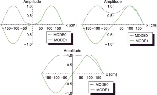
The space dependence of the static fluxes, showing the fundamental mode and the first higher-order mode is shown in Figure 4 for the three systems, starting with the loosely coupled system on to the strongly coupled system. These figures are in correspondence with similar results such as those in  [10,11,15,16].

Figure 4. Space dependence of the fundamental and first modes for the systems with various coupling properties (obtained by modifying Σ_{a, 2} in the second reactor region): loosely coupled (upper left figure), reference (upper right figure) and strongly coupled (bottom figure).

The frequency dependence of the corresponding modes is shown in Figure 5. The figure shows that, as expected, the amplitude of the fundamental mode, which is equal to the point kinetic component, diverges with decreasing frequencies. The behaviour of this mode is the same for all three systems. This is the generic behaviour in all critical systems subjected to a perturbation with a non-zero reactivity effect.

Figure 5. Frequency dependence of the amplitude of the fundamental and first mode components of the neutron noise for the systems with different coupling properties: loosely coupled (upper left figure), reference (upper right figure) and strongly coupled (bottom figure) (x = −120 cm, x_p = −150 cm).

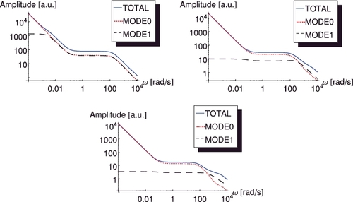
The behaviour of the first higher mode, on the other hand, is quite different in the loosely coupled system from that in the other two systems. In the reference and the strongly coupled systems, its amplitude is essentially constant below the plateau frequency, having actually the same value as at the plateau frequencies. In these systems, therefore, point kinetic behaviour is established quickly below the plateau frequency (in the strongly coupled system, actually the point kinetic component dominates even at plateau frequencies). For the loosely coupled system, on the other hand, the amplitude of the first mode shows the same increasing trend with decreasing frequency as the point reactor component over two orders of magnitude of the frequency below the plateau. In other words, such a system remains deeply space-dependent, with the first mode having comparable amplitude to that of the fundamental mode. Choosing an asymmetric perturbation with much smaller reactivity effect would even lead to the dominance of the first mode in such a system down to rather low frequencies.

It is also seen from the figures that the fundamental and first mode together make up for the total noise, and hence the contribution from the higher-order modes is negligible. Thus, it is seen that in a loosely coupled system with two coupled cores, the response essentially consists of the first two modes, and the contribution of the first higher-order mode to the system response is significant down to very low frequencies.

6. Conclusions

The simple considerations offered in this paper serve to illuminate the role of the ES in reactor dynamics and neutron noise theory. Through a simple example, it was shown how in a system of loosely coupled cores the smallness of the ES enhances the weight of the first higher-order mode in the system response which prevents the dominance of point kinetic behaviour down to very low frequencies. These considerations are in agreement with, and hence serve as confirmation of the origin and the characteristics of regional oscillations in a BWR.

Acknowledgements

One of the authors (I. Pázsit) wants to acknowledge valuable discussions with Prof. Kojiro Nishina of Nagoya University, who introduced him to the subject on his first visit to Japan in 1990. The authors are also greatly indebted to Prof. Yoshihiro Yamane for his valuable comments and advice on the manuscript. Financial support from JSPS for the visit of I. Pázsit is also highly appreciated (Grant No. JSPS/EP1/902S). This work was financially supported by the Ringhals power plant (Grant No. 663628-054).

Disclosure statement

No potential conflict of interest was reported by the authors.

Additional information

Funding

Financial support from JSPS for the visit of I. Pázsit is also highly appreciated (Grant No. JSPS/EP1/902S). This work was financially supported by the Ringhals power plant (Grant No. 663628-054).

Notes

1. Actually, for full consistency, ρ(ω) should also be denoted as δρ₀(ω). However, the zero index and the prefix δ was dropped because the notation ρ(ω) has been widely used for the traditional reactivity effect of a stationary perturbation. Hopefully this will not lead to any confusion.

2. For a spatial Dirac-delta type perturbation, the induced noise has a discontinuous space derivative in the point of perturbation. Thus, in general, a series expansion in terms of the static unperturbed eigenfunctions is not effective, due to slow convergence. However, even for such a case, at low frequencies, all higher order modes will be negligible compared to the first two modes.

References

- Stacey WM Jr.. Space-time nuclear reactor kinetics. New York (NY): Academic Press, Inc.; 1969.
- Rydin RA, Burke A, Moore WE, et al. Noise and transient kinetics experiments and calculations for loosely coupled cores. Nucl Sci Eng. 1971;46:179–196.
- Ebert DD, Clement J, Stacey WM Jr.. Investigation of the space- and energy-dependent coherence function in zero-power coupled-core reactors. Nucl Sci Eng. 1974;55:368–379.
- Ebert DD, Clement J, Stacey WM Jr.. Interpretation of coherence function measurements in zero-power coupled-core reactors. Nucl Sci Eng. 1974;55:380–386.
- Beckner WD, Rydin RA. Higher-order relationship between static power tilts and eigenvalue separation in nuclear-reactors. Nucl Sci Eng. 1975;56:131–141.
- Brumbach SB, Goin RW, Carpenter SG. Spatial kinetics studies in liquid-metal fast breeder reactor critical assemblies. Nucl Sci Eng. 1988;98:103–117.
- Sanda T. Interpretation of noise coherence function measurements in liquid-metal fast breeder reactor critical assemblies. Nucl Sci Eng. 1990;104:135–144.
- Hashimoto K, Ohsawa T, Miki R, et al. A practical formula for inferring eigenvalue separation from flux tilt measurements in nuclear-reactors. Ann Nucl Energy. 1991;18(3):131–140.
- Hashimoto K, Ohsawa T, Miki R, et al. Derivation of consistent reactivity worth and eigenvalue separation from space-dependent rod worths on the basis of modal approach. Ann Nucl Energy. 1991;18(6):317–325.
- Hashimoto K. Decoupling-phenomena, analyses of large nuclear reactor cores by the method of spatial higher harmonics [dissertation], Nagoya: Graduate School of Nuclear Engineering, Nagoya University; 1995, Japanese.
- Nishina K, Tokashiki M. Verification of more general correspondence between eigenvalue separation and coupling coefficient. Prog Nucl Energy. 1996;30:277–286.
- Andoh M, Misawa T, Nishina K, et al. Measurement of flux tilt and eigenvalue separation in axially decoupled core. J Nucl Sci Technol. 1997;34:445–453.
- Kato Y, Yamamoto T, Kitada T, et al. Analysis of first-harmonic eigenvalue separation experiments on KUCA coupled-core. J Nucl Sci Technol. 1998;35(3):216–225.
- Ishitani K, Yamane Y, Uritani A, et al. Measurement of eigenvalue separation by using position sensitive proportional counter. Ann Nucl Energy. 1998;25(10):721–732.
- Kobayashi K. A relation of the coupling coefficient to the eigenvalue separation in the coupled reactors theory. Ann Nucl Energy. 1998;25:189–201.
- Pyeon CH, Misawa S, Shiroya S, et al. Relationship between flux tilt in two-energy-group and eigenvalue separation. Ann Nucl Energy. 2001;28:1625–1641.
- Taninaka H, Hashimoto K, Pyeon CH, et al. Determination of lambda-mode eigenvalue separation of a thermal accelerator-driven system from pulsed neutron experiment. J Nucl Sci Technol. 2010;47(4):376–383.
- . In: Pázsit I, Demazière C. Cacuci DG. Noise techniques in nuclear systems, editor. Handbook of nuclear engineering. Vol. 3. New York (NY): Springer; 2010. p. 1631–1737.
- Dumonteil E, Courau T. Dominance ratio assessment and Monte Carlo criticality simulations: dealing with high dominance ratio systems. Nucl Technol. 2010;172:120–131.
- Kepisty G, Cetnar J. Dominance ratio evolution in large thermal reactors. Ann Nucl Energy. 2017;102:85–90.
- Pázsit I. Determination of reactor stability in case of dual oscillations. Ann Nucl Energy. 1995;22:377–387.
- Hashimoto K. Linear modal analysis of out-of-phase instability in boiling water reactor cores. Ann Nucl Energy. 1993;20:789–797.
- Hashimoto K, Hotta A, Takeda T. Neutronic model for modal multichannel analysis of out-of-phase instability in boiling water reactor cores. Ann Nucl Energy. 1997;24:99–111.
- Hotta A, Ninokata H, Takeuchi H, et al. Regional instability evaluation of Ringhals unit 1 based on extended frequency domain model. Nucl Eng Design. 2000;200:201–220.
- Ikeda H, Ama T, Hashimoto K, et al. Nonlinear behavior under regional neutron flux oscillations in BWR cores. J Nucl Sci Technol. 2001;38:312–323.
- McFarlane HF, Carpenter SG, Collins PJ, et al. Experimental studies of radially heterogeneous liquid-metal fast breeder reactor critical assemblies at the zero-power plutonium reactor. Nucl Sci Eng. 1984;87:204–232.
- Gialdi E, Grifoni S, Parmeggiani C, et al. Core stability in operating BWR: operational experience. Prog Nucl Energy. 1985;15:447–459.
- Vanderhagen THJJ, Pázsit I, Thomson O, et al. Methods for the determination of the in-phase and out-of-phase stability characteristics of a boiling water-reactor. Nucl Technol. 1994;107:193–214.
- Karlsson JKH, Pázsit I. Localisation of a channel instability in the Forsmark-1 boiling water reactor. Ann Nucl Energy. 1999;26:1183–1204.
- Pázsit I. Two-group theory of noise in reflected reactors with application to vibrating absorbers. Ann Nucl Energy. 1978;5:185–196.