Development of one-dimensional two-fluid model with consideration of void fraction covariance effect

ABSTRACT

Accurate evaluation of gas-liquid two-phase flow behavior within rod bundle geometry is crucial for the safety assessment of the nuclear power plants. In safety assessment codes, two-phase flow in rod bundle geometry has been treated as a one-dimensional flow. In order to obtain the reliable one-dimensional two-fluid model, it is essential to utilize proper area-averaged models for governing equations and constitutive relations. The area-averaged interfacial drag term utilized to evaluate two-phase interfacial drag force is typically given by the drift-flux parameters which consider the velocity profile in two-phase flow fields. However, in a rigorous sense, the covariance due to void fraction profile is ignored in traditional formulations. In this paper, the rigorous formulation of one-dimensional momentum equation was derived by taking consideration of void fraction covariance, and a new set of one-dimensional momentum equation and constitutive relations for interfacial drag was proposed. The newly obtained set of formulations was embedded into TRAC-BF1 code and numerical simulation was performed to compare against the traditional model without covariance. It was found that effect of covariance was almost negligible for steady-state adiabatic conditions, but for high void fraction condition with added perturbation, the traditional model underpredicted the damping ratio at around 8%.

KEYWORDS:

• 1D two-fluid model
• covariance
• momentum equation
• void fraction
• rod bundle

1. Introduction

In order to perform best-estimate safety evaluation for nuclear power plants, guidelines such as CSAU [1], V&V [2,3], and EMDAP [4] have been proposed to require (1) proper model selection, (2) reliability of the models, and (3) quantification of the model uncertainties utilized in numerical simulation codes [5]. Since coolant water also acts as a neutron moderator in the light-water reactor, to properly evaluate the safety of nuclear reactor, it is essential to develop thermal-hydraulic calculation models that were validated under the guidelines such as V&V.

In general, prediction of void fraction is categorized as one of the most important factors for the safety evaluation of nuclear reactors at a variety of scenarios and conditions. Especially for boiling-water reactor (BWR), two-phase flow behavior highly influences critical plant parameters such as core thermal power output, coolant pressure, core flow rate distribution, and so on. For example, significant parameters for the reactor safety evaluation such as Minimum Critical Power Ratio, maximum pressure value at pressure-boundary, Maximum Linear Heat Generation Rate, two-phase water level, and core stability damping ratio (DR), are highly sensitive to void fraction, and they are categorized as High-Rank in Phenomena Identification Ranking and Table.

In the two-fluid model utilized in one-dimensional system analysis code, momentum equation for each phase governs the phase velocity fields and they highly influence the void fraction prediction. Among the constitutive relations necessary for momentum equation closure, interfacial drag term has high sensitivity towards void fraction prediction. For the safety evaluation code for nuclear power plants such as TRACE [6], RELAP5 [7], and TRAC-BF1 [8], interfacial drag term proposed by Anderson and Chu [9] relates interfacial drag term with drift-flux parameters such as distribution parameter and drift velocity. In other words, interfacial drag expression is obtained by adapting the similar concept to the drift-flux model, which takes into consideration velocity distribution and void fraction distribution. Distribution parameter is defined based on spatial distribution of flow velocity and void fraction, and it is mainly influenced by the flow channel geometry. Ishii [10] developed the distribution parameter model for circular and rectangular channels, but for thermal-hydraulic analysis of reactor fuel assembly, the proper constitutive relation for rod bundle geometry is necessary. Ozaki and Hibiki [11,12] developed the drift-flux model for one-dimensional two-fluid model code based on the void fraction experimental database obtained at prototypic rod bundle geometry at actual range of operation condition. Hence, for drift-flux parameters, a reasonable prediction for core thermal-hydraulics should be possible by utilizing this model.

Interfacial drag term is derived from the force balance with respect to buoyancy force. However, to embed the term into one-dimensional system analysis code, covariance term due to void fraction distribution is necessary [13,14]. In traditional one-dimensional two-fluid model approach, covariance term is completely ignored in the area-averaged relative velocity term, as was presented by Ishii and Mishima [15]. Brooks et al. [14] pointed out that the area-averaged relative velocity without the covariance, namely Ishii and Mishima's formulation, may underestimate the area-averaged relative velocity considerably. Due to the necessity of accurate modeling for area-averaged relative velocity, Hibiki and Ozaki [16] developed the covariance model applicable for one-dimensional two-fluid model code based on the void fraction measurement data obtained at pipe flow under the scaled pressure condition based on prototypic PWR condition. Ozaki and Hibiki [17] also developed the covariance model based on the void fraction distribution measurement within prototypic rod bundle geometry. By merging the interfacial drag term with covariance effect into the one-dimensional two-fluid model, it is expected that more accurate and rigorous thermal-hydraulic analysis will be possible. However, the effect of the developed covariance models on thermal-hydraulic parameters such as void fraction has not been tested using a code.

As was shown, necessary constitutive relations for nuclear thermal-hydraulic simulation have been developed by various authors. In this paper, (1) modeling and modification of the momentum equation necessary for embedding new constitutive relations (related to void fraction covariance model proposed by Ozaki and Hibiki [17]) into one-dimensional two-fluid model, (2) comparison on code simulation results between models with and without covariance effect, and (3) evaluation of code performance in steady-state and transient conditions will be the main scope. It should be noted here that the covariance term is expected to affect the interfacial drag force, which may influence the damping of sudden flow parameter change.

2. Momentum equation in one-dimensional two-fluid model

Thermal-hydraulics in rod bundle geometry has been a challenging issue due to its geometrical complexity, difficulty in obtaining local constitutive formulations and validating the obtained experimental database. Hence, the problem has been treated as one-dimensional flow using area-averaged models and constitutive relations. For the numerical simulation in large-scale and complex flow geometry, it is necessary to conduct efficient calculation by optimizing the computational cost. Hence, the one-dimensional momentum equation utilized in system analysis code is obtained by area-averaging local momentum equation, and is given as follows [18]: (1) $$\begin{array}{ccc}& & ⟨{\alpha }_k⟩{\rho }_k\frac{\partial ⟨⟨v_k⟩⟩}{\partial t}+⟨{\alpha }_k⟩{\rho }_k⟨⟨v_k⟩⟩\frac{\partial ⟨⟨v_k⟩⟩}{\partial z}\hfill \\ & & =-⟨{\alpha }_k⟩\frac{\partial p}{\partial z}+⟨{\alpha }_k⟩⟨M_{\tau k}⟩-⟨{\alpha }_k⟩{\rho }_{k}g\hfill \\ & & +⟨M_{ik}⟩-\frac{4{\alpha }_{kw}{\tau }_{kw}}{D_h}\hfill \end{array}$$(1)

Here, subscript k denotes gas or liquid phase, and α_k, ρ_k, v_k, t, z, p, M_τk, g, M_ik, τ_kw, α_kw, and D_h, respectively, are the kth phase void fraction, density, velocity, time, axial position, pressure, viscous and turbulent shear stress, gravitational acceleration, interfacial drag, wall shear stress, void fraction near the wall, and hydraulic diameter. The symbols ⟨⟩ and ⟨⟨⟩⟩ are the area-averaging and void-weighted averaging operators.

2.1. Closure relations considering void fraction distribution

In order to close Equation (1)(1) $$\begin{array}{ccc}& & ⟨{\alpha }_k⟩{\rho }_k\frac{\partial ⟨⟨v_k⟩⟩}{\partial t}+⟨{\alpha }_k⟩{\rho }_k⟨⟨v_k⟩⟩\frac{\partial ⟨⟨v_k⟩⟩}{\partial z}\hfill \\ & & =-⟨{\alpha }_k⟩\frac{\partial p}{\partial z}+⟨{\alpha }_k⟩⟨M_{\tau k}⟩-⟨{\alpha }_k⟩{\rho }_{k}g\hfill \\ & & +⟨M_{ik}⟩-\frac{4{\alpha }_{kw}{\tau }_{kw}}{D_h}\hfill \end{array}$$(1) , constitutive relations are necessary for viscous and turbulent shear stress, interfacial drag and wall shear stress terms, respectively. Interfacial drag is obtained by the force balance with respect to buoyancy force, as shown in Equation (2)(2) $$\begin{array}{c}\hfill M_{ig}=-M_{if}=-{\alpha }_g{\alpha }_f\Delta \rho g\end{array}$$(2) (see Appendix). (2) $$\begin{array}{c}\hfill M_{ig}=-M_{if}=-{\alpha }_g{\alpha }_f\Delta \rho g\end{array}$$(2)

By area-averaging Equation (2)(2) $$\begin{array}{c}\hfill M_{ig}=-M_{if}=-{\alpha }_g{\alpha }_f\Delta \rho g\end{array}$$(2) , one obtains (3) $$\begin{array}{c}\hfill ⟨M_{ig}⟩=-⟨M_{if}⟩=-⟨{\alpha }_g⟩\left(1-C_{\alpha }⟨{\alpha }_g⟩\right)\Delta \rho g\end{array}$$(3)

Here, C_α is the covariance arose by area averaging void fraction, and is defined as shown in the following equation: (4) $$\begin{array}{c}\hfill C_{\alpha }\equiv \frac{〈{\alpha }_g^2〉}{⟨{\alpha }_g⟩⟨{\alpha }_g⟩}\end{array}$$(4)

The interfacial drag term is alternatively expressed in terms of the relative velocity between two phases (v_r), as shown in the following equation: (5) $$\begin{array}{c}\hfill M_{ig}=-M_{if}=-C_i\left|v_r\right|v_r\end{array}$$(5)

Here, C_i is the drag coefficient. Assuming uniform relative velocity profile across the flow channel, one obtains (6) $$\begin{array}{c}\hfill ⟨M_{ig}⟩=-⟨C_i⟩\left|⟨v_r⟩\right|⟨v_r⟩\end{array}$$(6)

From the relationship between Equations (3)(3) $$\begin{array}{c}\hfill ⟨M_{ig}⟩=-⟨M_{if}⟩=-⟨{\alpha }_g⟩\left(1-C_{\alpha }⟨{\alpha }_g⟩\right)\Delta \rho g\end{array}$$(3) and (6(6) $$\begin{array}{c}\hfill ⟨M_{ig}⟩=-⟨C_i⟩\left|⟨v_r⟩\right|⟨v_r⟩\end{array}$$(6) ), the drag coefficient is formulated as shown in the following equation: (7) $$\begin{array}{c}\hfill ⟨C_i⟩=\frac{⟨{\alpha }_g⟩\left(1-C_{\alpha }⟨{\alpha }_g⟩\right)\Delta \rho g}{{⟨v_r⟩}^2}\end{array}$$(7)

The area-averaged relative velocity term shown in the denominator of Equation (7)(7) $$\begin{array}{c}\hfill ⟨C_i⟩=\frac{⟨{\alpha }_g⟩\left(1-C_{\alpha }⟨{\alpha }_g⟩\right)\Delta \rho g}{{⟨v_r⟩}^2}\end{array}$$(7) can be re-expressed using drift velocity (v_gj) as follows [13,14]: (8) $$\begin{array}{c}\hfill ⟨v_r⟩=\frac{⟨⟨v_{gj}⟩⟩}{1-C_{\alpha }⟨{\alpha }_g⟩}\end{array}$$(8)

In addition, to express momentum coupling between two-phases, interfacial drag term should be related to phase velocity. Hence, the area-averaged relative velocity defined in Equation (9)(9) $$⟨v_r⟩=C_{\alpha }^{\text{'}}\left(\frac{1-C_0⟨{\alpha }_g⟩}{⟨{\alpha }_f⟩}⟨⟨v_g⟩⟩-C_0⟨⟨v_f⟩⟩\right)$$(9) will be substituted into the momentum equation [13,14]. (9) $$⟨v_r⟩=C_{\alpha }^{\text{'}}\left(\frac{1-C_0⟨{\alpha }_g⟩}{⟨{\alpha }_f⟩}⟨⟨v_g⟩⟩-C_0⟨⟨v_f⟩⟩\right)$$(9) (10) $$C_{\alpha }^{\text{'}}\equiv \frac{⟨{\alpha }_f⟩}{1-C_{\alpha }⟨{\alpha }_g⟩}$$(10)

Note that C₀ is the distribution parameter.

Substituting Equation (8)(8) $$\begin{array}{c}\hfill ⟨v_r⟩=\frac{⟨⟨v_{gj}⟩⟩}{1-C_{\alpha }⟨{\alpha }_g⟩}\end{array}$$(8) into Equation (7)(7) $$\begin{array}{c}\hfill ⟨C_i⟩=\frac{⟨{\alpha }_g⟩\left(1-C_{\alpha }⟨{\alpha }_g⟩\right)\Delta \rho g}{{⟨v_r⟩}^2}\end{array}$$(7) leads to the expression of the drag coefficient as follows: (11) $$\begin{array}{c}\hfill ⟨C_i⟩=\frac{⟨{\alpha }_g⟩{\left(1-C_{\alpha }⟨{\alpha }_g⟩\right)}^3\Delta \rho g}{{⟨⟨v_{gj}⟩⟩}^2}=\frac{1}{{{C^{\text{'}}}_{\alpha }}^3}\frac{⟨{\alpha }_g⟩{⟨{\alpha }_f⟩}^3\Delta \rho g}{{⟨⟨v_{gj}⟩⟩}^2}\end{array}$$(11)

Substituting the drag coefficient and Equation (9)(9) $$⟨v_r⟩=C_{\alpha }^{\text{'}}\left(\frac{1-C_0⟨{\alpha }_g⟩}{⟨{\alpha }_f⟩}⟨⟨v_g⟩⟩-C_0⟨⟨v_f⟩⟩\right)$$(9) into Equation (6)(6) $$\begin{array}{c}\hfill ⟨M_{ig}⟩=-⟨C_i⟩\left|⟨v_r⟩\right|⟨v_r⟩\end{array}$$(6) , one obtains the expression for area-averaged interfacial drag term as follows: (12) $$\begin{array}{ccc}\hfill ⟨M_{ig}⟩& =& -\frac{1}{{C^{\text{'}}}_{\alpha }}\frac{⟨{\alpha }_g⟩{⟨{\alpha }_f⟩}^3\Delta \rho g}{{⟨⟨v_{gj}⟩⟩}^2}\left(\frac{1-C_0⟨{\alpha }_g⟩}{⟨{\alpha }_f⟩}⟨⟨v_g⟩⟩-C_0⟨⟨v_f⟩⟩\right)\hfill \\ & & \times \left|\left(\frac{1-C_0⟨{\alpha }_g⟩}{⟨{\alpha }_f⟩}⟨⟨v_g⟩⟩-C_0⟨⟨v_f⟩⟩\right)\right|\hfill \end{array}$$(12)

Equation (12)(12) $$\begin{array}{ccc}\hfill ⟨M_{ig}⟩& =& -\frac{1}{{C^{\text{'}}}_{\alpha }}\frac{⟨{\alpha }_g⟩{⟨{\alpha }_f⟩}^3\Delta \rho g}{{⟨⟨v_{gj}⟩⟩}^2}\left(\frac{1-C_0⟨{\alpha }_g⟩}{⟨{\alpha }_f⟩}⟨⟨v_g⟩⟩-C_0⟨⟨v_f⟩⟩\right)\hfill \\ & & \times \left|\left(\frac{1-C_0⟨{\alpha }_g⟩}{⟨{\alpha }_f⟩}⟨⟨v_g⟩⟩-C_0⟨⟨v_f⟩⟩\right)\right|\hfill \end{array}$$(12) can be embedded into momentum equation along with the constitutive relations for distribution parameter, drift velocity, and covariance due to void fraction distribution.

Next, constitutive relations for viscous and turbulent shear stress will be discussed. Consider, non-accelerating steady-state two-phase flow condition, left-hand side of Equation (1)(1) $$\begin{array}{ccc}& & ⟨{\alpha }_k⟩{\rho }_k\frac{\partial ⟨⟨v_k⟩⟩}{\partial t}+⟨{\alpha }_k⟩{\rho }_k⟨⟨v_k⟩⟩\frac{\partial ⟨⟨v_k⟩⟩}{\partial z}\hfill \\ & & =-⟨{\alpha }_k⟩\frac{\partial p}{\partial z}+⟨{\alpha }_k⟩⟨M_{\tau k}⟩-⟨{\alpha }_k⟩{\rho }_{k}g\hfill \\ & & +⟨M_{ik}⟩-\frac{4{\alpha }_{kw}{\tau }_{kw}}{D_h}\hfill \end{array}$$(1) becomes zero. (13) $$\begin{array}{ccc}& & -⟨{\alpha }_g⟩\frac{\partial p}{\partial z}+⟨{\alpha }_g⟩⟨M_{\tau g}⟩-⟨{\alpha }_g⟩{\rho }_{g}g+⟨M_{ig}⟩\hfill \\ & & -\frac{4{\alpha }_{gw}{\tau }_{gw}}{D_h}=0\hfill \end{array}$$(13) (14) $$\begin{array}{ccc}& & -⟨{\alpha }_f⟩\frac{\partial p}{\partial z}+⟨{\alpha }_f⟩⟨M_{\tau f}⟩-⟨{\alpha }_f⟩{\rho }_{f}g-⟨M_{ig}⟩\hfill \\ & & -\frac{4{\alpha }_{fw}{\tau }_{fw}}{D_h}=0\hfill \end{array}$$(14)

Summation of Equations (13)(13) $$\begin{array}{ccc}& & -⟨{\alpha }_g⟩\frac{\partial p}{\partial z}+⟨{\alpha }_g⟩⟨M_{\tau g}⟩-⟨{\alpha }_g⟩{\rho }_{g}g+⟨M_{ig}⟩\hfill \\ & & -\frac{4{\alpha }_{gw}{\tau }_{gw}}{D_h}=0\hfill \end{array}$$(13) and (14(14) $$\begin{array}{ccc}& & -⟨{\alpha }_f⟩\frac{\partial p}{\partial z}+⟨{\alpha }_f⟩⟨M_{\tau f}⟩-⟨{\alpha }_f⟩{\rho }_{f}g-⟨M_{ig}⟩\hfill \\ & & -\frac{4{\alpha }_{fw}{\tau }_{fw}}{D_h}=0\hfill \end{array}$$(14) ) yields (15) $$\begin{array}{ccc}& & -\frac{\partial p}{\partial z}-{\rho }_{m}g+\left(⟨{\alpha }_g⟩⟨M_{\tau g}⟩-\frac{4{\alpha }_{gw}{\tau }_{gw}}{D_h}\right)\hfill \\ & & +\left(⟨{\alpha }_f⟩⟨M_{\tau f}⟩-\frac{4{\alpha }_{fw}{\tau }_{fw}}{D_h}\right)=0\hfill \end{array}$$(15)

Here, mixture density is defined as ρ_m = ⟨α_g⟩ρ_g + ⟨α_f⟩ρ_f. The two-phase pressure drop ($\partial p/\phantom{\partial p\partial z}\partial z$) term is obtained by adding wall friction and gravitational components, and the accelerational term can be assumed to be negligible. Then, Equation (16)(16) $$\begin{array}{ccc}& & \left(⟨{\alpha }_g⟩⟨M_{\tau g}⟩-\frac{4{\alpha }_{gw}{\tau }_{gw}}{D_h}\right)\hfill \\ & & +\left(⟨{\alpha }_f⟩⟨M_{\tau f}⟩-\frac{4{\alpha }_{fw}{\tau }_{fw}}{D_h}\right)=-F_w\hfill \end{array}$$(16) can be obtained which accounts for the viscous and turbulent shear stress, and wall shear stress terms. (16) $$\begin{array}{ccc}& & \left(⟨{\alpha }_g⟩⟨M_{\tau g}⟩-\frac{4{\alpha }_{gw}{\tau }_{gw}}{D_h}\right)\hfill \\ & & +\left(⟨{\alpha }_f⟩⟨M_{\tau f}⟩-\frac{4{\alpha }_{fw}{\tau }_{fw}}{D_h}\right)=-F_w\hfill \end{array}$$(16)

Here, F_w accounts for the pressure drop component due to two-phase wall frictional loss, and typically, it is given by the constitutive relations of single-phase friction factor and two-phase multiplier. On the other hand, Equation (17)(17) $$\begin{array}{ccc}& & ⟨{\alpha }_f⟩\left(⟨{\alpha }_g⟩⟨M_{\tau g}⟩-\frac{4{\alpha }_{gw}{\tau }_{gw}}{D_h}\right)\hfill \\ & & -⟨{\alpha }_g⟩\left(⟨{\alpha }_f⟩⟨M_{\tau f}⟩-\frac{4{\alpha }_{fw}{\tau }_{fw}}{D_h}\right)\hfill \\ & & ={⟨{\alpha }_g⟩}^2\Delta \rho g\left(1-C_{\alpha }\right)\hfill \end{array}$$(17) is obtained by eliminating pressure gradient term in Equations (13)(13) $$\begin{array}{ccc}& & -⟨{\alpha }_g⟩\frac{\partial p}{\partial z}+⟨{\alpha }_g⟩⟨M_{\tau g}⟩-⟨{\alpha }_g⟩{\rho }_{g}g+⟨M_{ig}⟩\hfill \\ & & -\frac{4{\alpha }_{gw}{\tau }_{gw}}{D_h}=0\hfill \end{array}$$(13) and (14(14) $$\begin{array}{ccc}& & -⟨{\alpha }_f⟩\frac{\partial p}{\partial z}+⟨{\alpha }_f⟩⟨M_{\tau f}⟩-⟨{\alpha }_f⟩{\rho }_{f}g-⟨M_{ig}⟩\hfill \\ & & -\frac{4{\alpha }_{fw}{\tau }_{fw}}{D_h}=0\hfill \end{array}$$(14) ). (17) $$\begin{array}{ccc}& & ⟨{\alpha }_f⟩\left(⟨{\alpha }_g⟩⟨M_{\tau g}⟩-\frac{4{\alpha }_{gw}{\tau }_{gw}}{D_h}\right)\hfill \\ & & -⟨{\alpha }_g⟩\left(⟨{\alpha }_f⟩⟨M_{\tau f}⟩-\frac{4{\alpha }_{fw}{\tau }_{fw}}{D_h}\right)\hfill \\ & & ={⟨{\alpha }_g⟩}^2\Delta \rho g\left(1-C_{\alpha }\right)\hfill \end{array}$$(17)

Here, Equation (3)(3) $$\begin{array}{c}\hfill ⟨M_{ig}⟩=-⟨M_{if}⟩=-⟨{\alpha }_g⟩\left(1-C_{\alpha }⟨{\alpha }_g⟩\right)\Delta \rho g\end{array}$$(3) was used for the interfacial drag term. Based on Equations (16)(16) $$\begin{array}{ccc}& & \left(⟨{\alpha }_g⟩⟨M_{\tau g}⟩-\frac{4{\alpha }_{gw}{\tau }_{gw}}{D_h}\right)\hfill \\ & & +\left(⟨{\alpha }_f⟩⟨M_{\tau f}⟩-\frac{4{\alpha }_{fw}{\tau }_{fw}}{D_h}\right)=-F_w\hfill \end{array}$$(16) and (17(17) $$\begin{array}{ccc}& & ⟨{\alpha }_f⟩\left(⟨{\alpha }_g⟩⟨M_{\tau g}⟩-\frac{4{\alpha }_{gw}{\tau }_{gw}}{D_h}\right)\hfill \\ & & -⟨{\alpha }_g⟩\left(⟨{\alpha }_f⟩⟨M_{\tau f}⟩-\frac{4{\alpha }_{fw}{\tau }_{fw}}{D_h}\right)\hfill \\ & & ={⟨{\alpha }_g⟩}^2\Delta \rho g\left(1-C_{\alpha }\right)\hfill \end{array}$$(17) ), viscous and turbulent shear stress, and wall shear stress terms can be derived as shown in Equations (18)(18) $$\begin{array}{ccc}& & \left(⟨{\alpha }_g⟩⟨M_{\tau g}⟩-\frac{4{\alpha }_{gw}{\tau }_{gw}}{D_h}\right)\hfill \\ & & =-⟨{\alpha }_g⟩F_w+{⟨{\alpha }_g⟩}^2\left(1-C_{\alpha }\right)\Delta \rho g\hfill \end{array}$$(18) and (19(19) $$\begin{array}{ccc}& & \left(⟨{\alpha }_f⟩⟨M_{\tau f}⟩-\frac{4{\alpha }_{fw}{\tau }_{fw}}{D_h}\right)\hfill \\ & & =-⟨{\alpha }_f⟩F_w-{⟨{\alpha }_g⟩}^2\left(1-C_{\alpha }\right)\Delta \rho g\hfill \end{array}$$(19) ). (18) $$\begin{array}{ccc}& & \left(⟨{\alpha }_g⟩⟨M_{\tau g}⟩-\frac{4{\alpha }_{gw}{\tau }_{gw}}{D_h}\right)\hfill \\ & & =-⟨{\alpha }_g⟩F_w+{⟨{\alpha }_g⟩}^2\left(1-C_{\alpha }\right)\Delta \rho g\hfill \end{array}$$(18) (19) $$\begin{array}{ccc}& & \left(⟨{\alpha }_f⟩⟨M_{\tau f}⟩-\frac{4{\alpha }_{fw}{\tau }_{fw}}{D_h}\right)\hfill \\ & & =-⟨{\alpha }_f⟩F_w-{⟨{\alpha }_g⟩}^2\left(1-C_{\alpha }\right)\Delta \rho g\hfill \end{array}$$(19)

Hence, closure relations for the momentum equation are completed by utilizing,

(1)

Viscous and turbulent shear stress, and wall shear stress terms that are obtained by substituting Equations (18)(18) $$\begin{array}{ccc}& & \left(⟨{\alpha }_g⟩⟨M_{\tau g}⟩-\frac{4{\alpha }_{gw}{\tau }_{gw}}{D_h}\right)\hfill \\ & & =-⟨{\alpha }_g⟩F_w+{⟨{\alpha }_g⟩}^2\left(1-C_{\alpha }\right)\Delta \rho g\hfill \end{array}$$(18) and (19(19) $$\begin{array}{ccc}& & \left(⟨{\alpha }_f⟩⟨M_{\tau f}⟩-\frac{4{\alpha }_{fw}{\tau }_{fw}}{D_h}\right)\hfill \\ & & =-⟨{\alpha }_f⟩F_w-{⟨{\alpha }_g⟩}^2\left(1-C_{\alpha }\right)\Delta \rho g\hfill \end{array}$$(19) ) into Equation (1)(1) $$\begin{array}{ccc}& & ⟨{\alpha }_k⟩{\rho }_k\frac{\partial ⟨⟨v_k⟩⟩}{\partial t}+⟨{\alpha }_k⟩{\rho }_k⟨⟨v_k⟩⟩\frac{\partial ⟨⟨v_k⟩⟩}{\partial z}\hfill \\ & & =-⟨{\alpha }_k⟩\frac{\partial p}{\partial z}+⟨{\alpha }_k⟩⟨M_{\tau k}⟩-⟨{\alpha }_k⟩{\rho }_{k}g\hfill \\ & & +⟨M_{ik}⟩-\frac{4{\alpha }_{kw}{\tau }_{kw}}{D_h}\hfill \end{array}$$(1) , and

(2)

Interfacial drag term defined in Equation (12)(12) $$\begin{array}{ccc}\hfill ⟨M_{ig}⟩& =& -\frac{1}{{C^{\text{'}}}_{\alpha }}\frac{⟨{\alpha }_g⟩{⟨{\alpha }_f⟩}^3\Delta \rho g}{{⟨⟨v_{gj}⟩⟩}^2}\left(\frac{1-C_0⟨{\alpha }_g⟩}{⟨{\alpha }_f⟩}⟨⟨v_g⟩⟩-C_0⟨⟨v_f⟩⟩\right)\hfill \\ & & \times \left|\left(\frac{1-C_0⟨{\alpha }_g⟩}{⟨{\alpha }_f⟩}⟨⟨v_g⟩⟩-C_0⟨⟨v_f⟩⟩\right)\right|\hfill \end{array}$$(12) .

Constitutive correlations in the present study are detailed in Section 3.1.1.

2.2. Closure relations for uniform void fraction assumption

Area averaging the interfacial drag term defined in Equation (2)(2) $$\begin{array}{c}\hfill M_{ig}=-M_{if}=-{\alpha }_g{\alpha }_f\Delta \rho g\end{array}$$(2) assuming uniform void fraction distribution leads to the expression shown in the following equation: (20) $$\begin{array}{c}\hfill ⟨M_{ig}⟩=-⟨M_{if}⟩=-⟨{\alpha }_g⟩⟨{\alpha }_f⟩\Delta \rho g\end{array}$$(20)

As was shown in Section 2.1, utilizing Equation (6)(6) $$\begin{array}{c}\hfill ⟨M_{ig}⟩=-⟨C_i⟩\left|⟨v_r⟩\right|⟨v_r⟩\end{array}$$(6) for the relationship between interfacial drag and relative velocity, drag coefficient under uniform void profile assumption is derived as (21) $$\begin{array}{c}\hfill ⟨C_i⟩=\frac{⟨{\alpha }_g⟩⟨{\alpha }_f⟩\Delta \rho g}{{⟨v_r⟩}^2}\end{array}$$(21)

In contrast to Equation (8)(8) $$\begin{array}{c}\hfill ⟨v_r⟩=\frac{⟨⟨v_{gj}⟩⟩}{1-C_{\alpha }⟨{\alpha }_g⟩}\end{array}$$(8) , the relationship between relative velocity and drift velocity is given as (22) $$\begin{array}{c}\hfill ⟨v_r⟩=\frac{⟨⟨v_{gj}⟩⟩}{⟨{\alpha }_f⟩}\end{array}$$(22)

The relationship between relative velocity and field velocity, which corresponds to Equation (9)(9) $$⟨v_r⟩=C_{\alpha }^{\text{'}}\left(\frac{1-C_0⟨{\alpha }_g⟩}{⟨{\alpha }_f⟩}⟨⟨v_g⟩⟩-C_0⟨⟨v_f⟩⟩\right)$$(9) , is given as (23) $$\begin{array}{c}\hfill ⟨v_r⟩=\frac{1-C_0⟨{\alpha }_g⟩}{⟨{\alpha }_f⟩}⟨⟨v_g⟩⟩-C_0⟨⟨v_f⟩⟩\end{array}$$(23)

Hence, for the uniform void profile assumption, area-averaged interfacial drag term defined in Equation (12)(12) $$\begin{array}{ccc}\hfill ⟨M_{ig}⟩& =& -\frac{1}{{C^{\text{'}}}_{\alpha }}\frac{⟨{\alpha }_g⟩{⟨{\alpha }_f⟩}^3\Delta \rho g}{{⟨⟨v_{gj}⟩⟩}^2}\left(\frac{1-C_0⟨{\alpha }_g⟩}{⟨{\alpha }_f⟩}⟨⟨v_g⟩⟩-C_0⟨⟨v_f⟩⟩\right)\hfill \\ & & \times \left|\left(\frac{1-C_0⟨{\alpha }_g⟩}{⟨{\alpha }_f⟩}⟨⟨v_g⟩⟩-C_0⟨⟨v_f⟩⟩\right)\right|\hfill \end{array}$$(12) can be expressed as (24) $$\begin{array}{ccc}\hfill ⟨M_{ig}⟩& =& -\frac{⟨{\alpha }_g⟩{⟨{\alpha }_f⟩}^3\Delta \rho g}{{⟨⟨v_{gj}⟩⟩}^2}\left|\frac{1-C_0⟨{\alpha }_g⟩}{⟨{\alpha }_f⟩}⟨⟨v_g⟩⟩-C_0⟨⟨v_f⟩⟩\right|\hfill \\ & & \times \left(\frac{1-C_0⟨{\alpha }_g⟩}{⟨{\alpha }_f⟩}⟨⟨v_g⟩⟩-C_0⟨⟨v_f⟩⟩\right)\hfill \end{array}$$(24)

As shown in Equation (23)(23) $$\begin{array}{c}\hfill ⟨v_r⟩=\frac{1-C_0⟨{\alpha }_g⟩}{⟨{\alpha }_f⟩}⟨⟨v_g⟩⟩-C_0⟨⟨v_f⟩⟩\end{array}$$(23) , it is obtained by simplifying Equation (9)(9) $$⟨v_r⟩=C_{\alpha }^{\text{'}}\left(\frac{1-C_0⟨{\alpha }_g⟩}{⟨{\alpha }_f⟩}⟨⟨v_g⟩⟩-C_0⟨⟨v_f⟩⟩\right)$$(9) with C_α = 1 assumption. Similarly, C₀ should be ideally equal to 1 for the uniform void profile assumption, but as is the case for the simulation code, it is given by the constitutive relation. It is worthy of note that while emphasizing the importance of void profile distribution, setting C_α = 1 largely contradicts the problem-solving approach and lacks consistency.

For viscous and turbulent stress terms, and wall shear stress term, Equations (15)(15) $$\begin{array}{ccc}& & -\frac{\partial p}{\partial z}-{\rho }_{m}g+\left(⟨{\alpha }_g⟩⟨M_{\tau g}⟩-\frac{4{\alpha }_{gw}{\tau }_{gw}}{D_h}\right)\hfill \\ & & +\left(⟨{\alpha }_f⟩⟨M_{\tau f}⟩-\frac{4{\alpha }_{fw}{\tau }_{fw}}{D_h}\right)=0\hfill \end{array}$$(15) and (16(16) $$\begin{array}{ccc}& & \left(⟨{\alpha }_g⟩⟨M_{\tau g}⟩-\frac{4{\alpha }_{gw}{\tau }_{gw}}{D_h}\right)\hfill \\ & & +\left(⟨{\alpha }_f⟩⟨M_{\tau f}⟩-\frac{4{\alpha }_{fw}{\tau }_{fw}}{D_h}\right)=-F_w\hfill \end{array}$$(16) ) still hold for uniform void profile assumption with a non-accelerating steady-state condition. On the other hand, for Equation (17)(17) $$\begin{array}{ccc}& & ⟨{\alpha }_f⟩\left(⟨{\alpha }_g⟩⟨M_{\tau g}⟩-\frac{4{\alpha }_{gw}{\tau }_{gw}}{D_h}\right)\hfill \\ & & -⟨{\alpha }_g⟩\left(⟨{\alpha }_f⟩⟨M_{\tau f}⟩-\frac{4{\alpha }_{fw}{\tau }_{fw}}{D_h}\right)\hfill \\ & & ={⟨{\alpha }_g⟩}^2\Delta \rho g\left(1-C_{\alpha }\right)\hfill \end{array}$$(17) , Equation (25)(25) $$\begin{array}{ccc}& & ⟨{\alpha }_f⟩\left(⟨{\alpha }_g⟩⟨M_{\tau g}⟩-\frac{4{\alpha }_{gw}{\tau }_{gw}}{D_h}\right)\hfill \\ & & -⟨{\alpha }_g⟩\left(⟨{\alpha }_f⟩⟨M_{\tau f}⟩-\frac{4{\alpha }_{fw}{\tau }_{fw}}{D_h}\right)=0\hfill \end{array}$$(25) is obtained by substituting interfacial drag term defined in Equation (20)(20) $$\begin{array}{c}\hfill ⟨M_{ig}⟩=-⟨M_{if}⟩=-⟨{\alpha }_g⟩⟨{\alpha }_f⟩\Delta \rho g\end{array}$$(20) . (25) $$\begin{array}{ccc}& & ⟨{\alpha }_f⟩\left(⟨{\alpha }_g⟩⟨M_{\tau g}⟩-\frac{4{\alpha }_{gw}{\tau }_{gw}}{D_h}\right)\hfill \\ & & -⟨{\alpha }_g⟩\left(⟨{\alpha }_f⟩⟨M_{\tau f}⟩-\frac{4{\alpha }_{fw}{\tau }_{fw}}{D_h}\right)=0\hfill \end{array}$$(25)

Hence, for uniform void profile assumption, viscous and turbulent stresses and wall shear stress terms for gas and liquid phases are given as follows: (26) $$\begin{array}{c}\hfill \left(⟨{\alpha }_g⟩⟨M_{\tau g}⟩-\frac{4{\alpha }_{gw}{\tau }_{gw}}{D_h}\right)=-⟨{\alpha }_g⟩F_w\end{array}$$(26) (27) $$\begin{array}{c}\hfill \left(⟨{\alpha }_f⟩⟨M_{\tau f}⟩-\frac{4{\alpha }_{fw}{\tau }_{fw}}{D_h}\right)=-⟨{\alpha }_f⟩F_w\end{array}$$(27)

As was shown, uniform void profile assumption lacks consistency, since it still utilizes distribution parameter which put emphasize on the relative velocity and void fraction distributions.

It should be noted here that the interfacial drag force model is formulated by the drift-flux correlation developed under steady-state conditions. Since a bubbly in water reaches its terminal velocity within a few ten milliseconds [19], the steady-state assumption is acceptable for simulation slow transient phenomena. However, the applicability of the code with the interfacial drag force model for transient conditions should be validated.

3. Effect on code calculation due to approximations

For one-dimensional system analysis code such as TRACE and TRAC-BF1, momentum equation derived under uniform void profile assumption (Section 2.2) is commonly utilized, and the expression deviates from the rigorous and detailed formulation with void fraction covariance (Section 2.1). In addition, void fraction covariance has an effect on area-averaged relative velocity term, but the current system analysis code still assumes uniform void distribution. When considering the effect of void distribution, it is necessary to supply covariance term. Due to the advancement of the instrumentations, such as conductivity probe for local void fraction measurement [20–24], void fraction distribution measurement using X-ray CT scanner [25], and so on, development of the covariance model for the void profile is now possible [13,14,16,17]. For the safety assessment of the nuclear power plant, validity of the thermal-hydraulic simulation at reactor core region becomes crucial. Hence, in the following chapter, thermal-hydraulic analysis within fuel rod bundle using TRAC-BF1 code will be demonstrated to evaluate the effect on uniform void distribution assumption.

3.1. Code model (constitutive relations) and calculation conditions

3.1.1. Constitutive relations

In order to close the momentum equation, it is necessary to supply constitutive relations for (1) distribution parameter, (2) drift velocity, (3) void fraction covariance and, (4) wall frictional pressure loss, are necessary. In this paper, appropriateness of fore mentioned constitutive relations that are related to void distribution will be assessed. They are tabulated in Table 1, and each category is summarized in the following:

(1)	Distribution parameter model

Table 1. Constitutive equations implemented in TRAC-BF1 code

Item	Model
Distribution parameter, C0	$C_0=1.1-0.1\sqrt{\frac{{\rho }_g}{{\rho }_f}},\mathrm{for}\mathrm{bulk}\mathrm{boiling}\mathrm{condition}$ [11, 12]
	$C_0=\left(1.1-0.1\sqrt{\frac{{\rho }_g}{{\rho }_f}}\right)\left(1-e^{-12.1{⟨{\alpha }_g⟩}^{0.701}}\right),\mathrm{for}\mathrm{sub}\text{-}\mathrm{cooled}\mathrm{boiling}\mathrm{condition}$ [17]
Drift velocity, ⟨⟨vgj⟩⟩	$\begin{array}{c}⟨⟨V_{gj}^{+}⟩⟩+⟨⟨V_{gj,B}^{+}⟩⟩exp\left(-1.39⟨J_g^{+}⟩\right)+⟨V_{gj,P}^{+}⟩\left\{1-exp\left(-1.39⟨J_g^{+}⟩\right)\right\}\hfill \end{array}\left[26\right]$
	$⟨V_{gj,B}^{+}⟩=\sqrt{2}{\left(1-⟨\alpha ⟩\right)}^{1.75}\left[10\right]$
	$\begin{array}{c}\mathrm{when}{N}_{uf}\le 2.25\times {10}^{-8}\hfill \\ ⟨⟨V_{gj,P}^{+}⟩⟩=0.0019{\left(D_H^{+}\right)}^{0.809}{\left(\frac{{\rho }_g}{{\rho }_f}\right)}^{-0.157}{N}_{\mu f}^{-0.562}for{D}_H^{+}\le 30\hfill \\ ⟨⟨V_{gj,P}^{+}⟩⟩=0.030{\left(\frac{{\rho }_g}{{\rho }_f}\right)}^{-0.562}{N}_{\mu f}^{-0.562}for{D}_H^{+}\ge 30\hfill \\ \mathrm{when}{N}_{\mu f}\ge 2.25\times {10}^{-3}\hfill \\ ⟨⟨V_{gj,P}^{+}⟩⟩=0.92{\left(\frac{{\rho }_g}{{\rho }_f}\right)}^{-0.157}\mathrm{for}{D}_H^{+}\ge 30\left[27\right]\hfill \end{array}$
	$⟨⟨V_{gj}^{+}⟩⟩=\frac{⟨⟨v_{gj}⟩⟩}{{\left(\frac{\sigma g\Delta \rho }{{\rho }_f^2}\right)}^{1/4}},⟨j_g^{+}⟩=\frac{⟨j_g⟩}{{\left(\frac{\sigma g\Delta \rho }{{\rho }_f^2}\right)}^{1/4}},D_H^{+}=\frac{D_H}{\sqrt{\frac{\sigma }{g\Delta \rho }}},N_{\mu f}=\frac{{\mu }_f}{{\left({\rho }_f\sigma \sqrt{\frac{\sigma }{g\Delta \rho }}\right)}^{1/2}}$
Void fraction covariance, Cα	$C_{\alpha ,\mathrm{BB}}=1+\left\{9.38{\left(⟨{\alpha }_g⟩-0.5\right)}^4+0.414\right\}\left\{1-{\left(\frac{{\rho }_g}{{\rho }_f}\right)}^2\right\}⟨{\alpha }_f⟩$ [17]
	$C_{\alpha ,\mathrm{SB}}=\frac{0.190}{{⟨{\alpha }_g⟩}^{0.855}}$ [17]
	Cα(⟨αg⟩) = max (Cα, SB, Cα, BB)for⟨αcrit⟩ > ⟨αg⟩
	$C_{\alpha }\left(⟨{\alpha }_g⟩\right)=\frac{1-C_{\alpha }\left(⟨{\alpha }_{\mathrm{crit}}⟩\right)}{1-\left(⟨{\alpha }_{\mathrm{crit}}⟩\right)}\left(⟨{\alpha }_g⟩-1\right)+1\mathrm{for}⟨{\alpha }_{\mathrm{crit}}⟩\le ⟨{\alpha }_g⟩$
	⟨αcrit⟩ = 0.84

The distribution parameter model proposed by Ozaki and Hibiki [11,12] is utilized. This model was developed based on the void fraction database obtained at rod bundle geometry under prototypic BWR operation condition. Additionally, Ozaki and Hibiki's [17] model was developed using bubble layer thickness model, which is applicable for sub-cooled flow boiling case. Hence, one of the advantages to use this model is that numerical discontinuity between sub-cooled and bulk boiling can be avoided.

• (2) Drift velocity model

For the drift velocity model, Hibiki–Ishii model [26] is utilized. The model was developed based on the Ishii's [10] drift velocity model under bubbly flow condition, and Kataoka and Ishii's [27] model under pool and large-diameter pipe flow conditions. The model is applicable for rod bundle geometry [11,12].

• (3) Covariance model for void fraction distribution

Ozaki and Hibiki's model [17] is utilized for void fraction distribution covariance. Since covariance is affected by wall conditions as well as the distribution parameter, it is necessary to utilize the model that was developed under void fraction database on rod bundle geometry. Ozaki and Hibiki [17] developed covariance model for bulk boiling condition based on the void fraction distribution database using X-ray CT scanner obtained at NUPEC's rod bundle geometry [25,28,29]. In addition, covariance model under sub-cooled boiling condition was also developed by adopting bubble-layer-thickness model; hence, it can cover wide range of void fraction under sub-cooled to bulk boiling conditions. The relationship between void fraction and covariance obtained using Ozakin and Hibiki [17] is depicted in Figure 1. As shown in the plot, the condition C_α ⩾ 1 is satisfied for entire void fraction range, but at high void fraction value close to churn-annular flow transition region, covariance approaches to large value. Hence, it can be said that effect of void fraction distribution becomes noticeable at high void fraction region close to churn-annular flow transition region.

• (4) Wall frictional pressure loss

The constitutive correlation based on Moody diagram [30] is used for calculating single-phase wall frictional pressure loss, whereas the constitutive correlation based on Martinelli–Nelson model [31] is adopted for calculating two-phase wall frictional pressure loss. It should be noted here that the pressure losses due to space grids is not considered in code calculations because reference void fraction is computed under hypothetical bundle without space grids.

Figure 1. Void fraction covariance and relative velocity covariance calculated by Ozaki and Hibiki [17] model at a pressure of 7 MPa.

3.1.2. Calculation condition

As can be seen from the derivations shown in the previous section, the interfacial drag model and calculated area-averaged void fraction value are highly related to one another. Hence, in this paper, an effect of void distribution treatments (with and without covariance) on the area-averaged void fraction in rod bundle geometry is investigated.

Figure 2 shows the calculation domain used in the TRAC-BF1 analysis. As shown in the figure, CHAN component which utilizes constitutive relations for rod bundle geometry was used to simulate the 8 × 8 rod bundle two-phase flow. The overall length of CHAN component was set to 5 m and they were evenly divided into 50 cells. The upstream 2.4 m segment of CHAN component was set to uniform-heat generation cell, and two-phase flow condition was simulated with vapor generated via wall-heating. Note that the upstream component that acts as an inlet cell was set to an adiabatic condition. The downstream 25 cells with an overall length of 2.5 m were set to adiabatic condition, and steady-state two-phase flow condition without phase change was simulated.

Figure 2. Calculation model and nodalization of TRAC-BF1 for rod bundle under two-phase flow (steady-state simulation case).

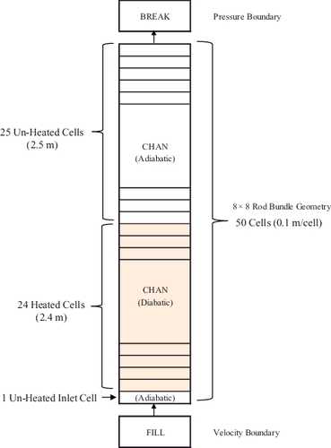
The downstream of CHAN component was connected to BREAK component, which sets a pressure boundary value, and BWR's operation condition of 7 MPa was assigned. In addition, upstream of the CHAN component was connected to FILL component, which sets flow rate and temperature boundary value, and inlet sub-cooling was set to about 50 kJ/kg. The thermal power output for the uniform heating section was calculated by solving for the corresponding void fraction value. By defining the void fraction value as ⟨α_g⟩_target, exit flow quality at heating section ⟨x_f⟩_exit can be calculated using drift-flux model [32] using following relation: (28) $$\begin{array}{c}\hfill {⟨{\alpha }_g⟩}_{\mathrm{target}}=\frac{{⟨x_f⟩}_{\mathrm{exit}}}{C_0\left[{⟨x_f⟩}_{\mathrm{exit}}+\left(1-{⟨x_f⟩}_{\mathrm{exit}}\right)\frac{{\rho }_g}{{\rho }_f}\right]+\frac{{\rho }_g⟨⟨v_{gj}⟩⟩}{G}}\end{array}$$(28)

Here, G represents mass flux. If saturation condition was assumed at the exit of heating section, flow quality becomes identical to thermal equilibrium quality. Therefore, required heat generation value can be obtained from⟨α_g⟩_target and inlet enthalpy value. As can be seen from Figure 1, since covariance tends to be larger at high area-averaged void fraction region, ⟨α_g⟩_target was set to high value and effect of void fraction covariance was investigated.

4. Results and discussions

4.1. Steady-state condition

For the steady-state analysis, void fraction calculation results for rod bundle geometry was obtained once by setting inlet and outlet boundary conditions and bundle power output value as constant. The target void fraction value was set to 0.8, and nine inlet conditions with inlet flow rate ranging from 1.5 to 15 kg/s were considered. For the exit condition, the drift-flux model was utilized to obtain exit void fraction value equivalent to ⟨α_g⟩_target. Inlet and outlet boundary conditions and bundle power output values are tabulated in Table 2.

Table 2. Boundary conditions of inlet flow rate, outlet pressure and bundle power conditions for steady-state simulations

Run	Inlet mass	Mass flux in	Outlet pressure	Bundle power
no.	flow rate (kg/s)	bundle (kg/m^2s)	(MPa)	(MW)
1	1.5	154	7.0	1.5
2	2.0	205	7.0	1.7
3	2.5	256	7.0	1.9
4	3.0	308	7.0	2.1
5	3.5	359	7.0	2.3
6	4.0	410	7.0	2.5
7	5.0	513	7.0	2.9
8	10.0	1025	7.0	4.9
9	15.0	1538	7.0	6.9

Figure 3 shows the area-averaged void fraction calculated at the non-heated section with the inlet flow conditions of 5, 10, 15 kg/s (Run 7, 8, and 9). Calculation results of two cases, with uniform void fraction distribution (without covariance) and void fraction covariance (with covariance), are plotted in the figure.

Figure 3. Comparisons of axial void fraction profiles for steady-state simulation cases at targeted void fraction of 0.8 and mass flow rate of (a) 5, (b) 10, and (c) 15 kg/s.

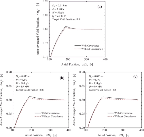
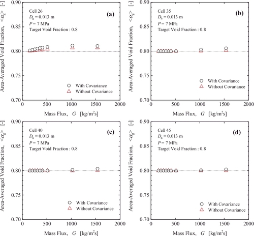
As can be seen from the figure, area-averaged void fraction value tends to increase with vapor generation in the heated region. Due to the vapor generation and diffusion terms, the exit void fraction value at the heated region overestimated targeted void fraction value of 0.8, but it approaches targeted void fraction value near the exit of rod bundle section. Such void fraction overestimation tends to be larger at downstream of heated region, but it quickly reaches the targeted void fraction value in the case of low mass flow rate condition. On the other hand, at high mass flow rate condition, longer distance requires approaching targeted void fraction value because of large convection effect. In order to compare calculated results against targeted void fraction value, the relationship between area-averaged void fraction and mass flux was plotted in Figure 4 for the downstream of heated-segment (cell #, 26, 35, 40, and 45). As can be seen from the plot, for both of void distribution treatments, calculation results obtained by the two-fluid model code is close to the targeted void fraction value obtained by the drift-flux model. Comparing the area-averaged void fraction values for both cases, a very small difference was confirmed (within 1%). For the case of void fraction covariance, void fraction overestimation at the exit of heated-region tends to be larger compared to the case with uniform void distribution. Summation of the source terms in right-hand-side of momentum equation matches for both cases, and interfacial drag term tends to be smaller for the void fraction covariance case, as shown in Equations (12)(12) $$\begin{array}{ccc}\hfill ⟨M_{ig}⟩& =& -\frac{1}{{C^{\text{'}}}_{\alpha }}\frac{⟨{\alpha }_g⟩{⟨{\alpha }_f⟩}^3\Delta \rho g}{{⟨⟨v_{gj}⟩⟩}^2}\left(\frac{1-C_0⟨{\alpha }_g⟩}{⟨{\alpha }_f⟩}⟨⟨v_g⟩⟩-C_0⟨⟨v_f⟩⟩\right)\hfill \\ & & \times \left|\left(\frac{1-C_0⟨{\alpha }_g⟩}{⟨{\alpha }_f⟩}⟨⟨v_g⟩⟩-C_0⟨⟨v_f⟩⟩\right)\right|\hfill \end{array}$$(12) and (24(24) $$\begin{array}{ccc}\hfill ⟨M_{ig}⟩& =& -\frac{⟨{\alpha }_g⟩{⟨{\alpha }_f⟩}^3\Delta \rho g}{{⟨⟨v_{gj}⟩⟩}^2}\left|\frac{1-C_0⟨{\alpha }_g⟩}{⟨{\alpha }_f⟩}⟨⟨v_g⟩⟩-C_0⟨⟨v_f⟩⟩\right|\hfill \\ & & \times \left(\frac{1-C_0⟨{\alpha }_g⟩}{⟨{\alpha }_f⟩}⟨⟨v_g⟩⟩-C_0⟨⟨v_f⟩⟩\right)\hfill \end{array}$$(24) ). Hence, due to the weak binding of phase velocity for covariance case, additional distance is required to fully recover the void fraction overestimation.

Figure 4. Comparisons of the void fraction at (a) 26th cell, (b) 35th cell, (c) 40th cell, and (d) 45th cell from the inlet of CHAN component with the conditions of mass flux.

4.2. Transient condition

As was shown in Chapter 2, the case with void fraction covariance tends to weaken the momentum coupling between gas–liquid two phases. For non-accelerating steady-state condition, the results of two cases were found to be identical, as was shown in Section 4.1. However, for a transient condition, a weakly coupled two-phase formulation may result in the difference in area-averaged void fraction calculation. For the transient condition, two-phase stability problem will be focused in the current study. It is well known that two-phase instability phenomenon arises when an external disturbance is added to the flow channel of constant hydraulic head [33]. As shown in Figure 5, inlet boundary was changed to BREAK component, and both upstream and downstream pressure values were set to create a constant hydraulic-head condition. Under such boundary conditions, bundle power output of CHAN component was adjusted, and change in area-averaged void fraction and inlet flow rate with respect to time was assessed for the two cases. The upstream and downstream boundary conditions and initial conditions are tabulated in Table 3. Figure 6 depicts the rated power behavior with respect to time. Here, the differential pressure between upstream and downstream is adjusted to set 10 kg/s mass flow rate in an initial state. Also, since covariance term is highly dependent on void fraction value, several calculation cases with different initial void fraction condition were considered in this analysis. The ramp rate such as 1.4 times increase during the period from 1 to 3 s is determined to maximize the covariance effect on the void fraction in the code calculation.

Figure 5. Calculation model and nodalization of TRAC-BF1 for rod bundle under two-phase flow (transient simulation case).

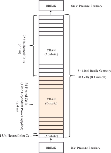
Table 3. Pressure boundary conditions and initial power and void fraction conditions for transient simulations

Run	Inlet pressure	Outlet pressure	Initial bundle	Initial targeted outlet
no.	(MPa)	(MPa)	power (MW)	void fraction (-)
10	7.04	7.0	1.15	0.4
11	7.04	7.0	1.50	0.5
12	7.04	7.0	2.03	0.6
13	7.05	7.0	2.95	0.7

Figure 6. Bundle power perturbation applied for transient simulation case.

Change in an area-averaged void fraction with respect to time at 45th cell counting from the upstream of CHAN component is plotted in Figure 7, and change in mass flow rate with respect to time at the first cell from the upstream of CHAN component is plotted in Figure 8. Initial void fraction and inlet flow rate were set to 0.7, and 10 kg/s, respectively, and it is identical to the steady-state condition until the perturbation is added to the system. As shown in Figure 6, bundle power perturbation is added after 1 s, and void fraction and two-phase pressure drop within rod bundle tend to increase. This results in a decrease in inlet flow rate at constant differential pressure condition. Following the decrease in power output after 2 s, void fraction tends to decrease. Similarly, inlet flow rate tends to increase, but it overshoots the initial condition, and oscillatory behavior is initiated. As shown in the figures, similar behaviors were observed for both cases with and without covariance, but the oscillation decays much faster for the uniform void distribution case. The drag coefficient for the case without the covariance is smaller than that for the case with the covariance. The interfacial drag force stabilizes the oscillation. Therefore, the smaller drag coefficient for the case without the covariance results in the larger amplitude and the longer period of the oscillation. In order to evaluate such oscillatory behaviors, DR is now introduced for the analysis. (29) $$\begin{array}{c}\hfill \mathrm{DR}=\frac{X_{+4}-X_{\mathrm{steady}}}{X_{+3}-X_{\mathrm{steady}}}\end{array}$$(29)

Figure 7. Comparison of area-averaged void fraction trend at the 45th cell from the inlet of CHAN component.

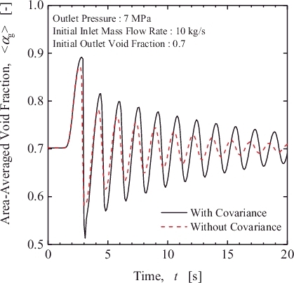
Figure 8. Comparison of inlet flow rate of CHAN component.

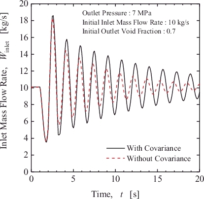
Here, X is the parameter of interest, such as void fraction or inlet flow rate, and subscript +4, +3, and steady are the fourth positive peak, third positive peak, and steady-state condition, respectively. The time of positive second peaks, about 3.5 s shown in Figures 7 and 8, are close to the time of the end of power perturbation, 3 s. Therefore, this external initial disturbance may affect the amplitude of the positive second peaks. Consequently, third and fourth peaks are selected for the representative peak values since these peaks are not affected by the initial disturbance.

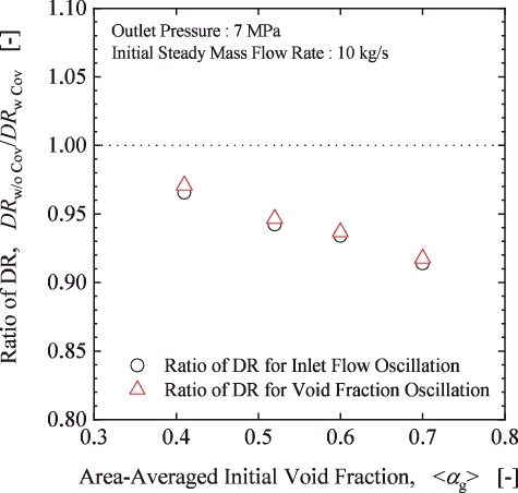
Figure 9 shows the calculation results from the conditions shown in Table 3. For each condition, DR was obtained at given void fraction and inlet flow rate, and it was compared for both cases with and without covariance. The dumping behavior is affected by the magnitude of interfacial drag term expressed by Equation (12)(12) $$\begin{array}{ccc}\hfill ⟨M_{ig}⟩& =& -\frac{1}{{C^{\text{'}}}_{\alpha }}\frac{⟨{\alpha }_g⟩{⟨{\alpha }_f⟩}^3\Delta \rho g}{{⟨⟨v_{gj}⟩⟩}^2}\left(\frac{1-C_0⟨{\alpha }_g⟩}{⟨{\alpha }_f⟩}⟨⟨v_g⟩⟩-C_0⟨⟨v_f⟩⟩\right)\hfill \\ & & \times \left|\left(\frac{1-C_0⟨{\alpha }_g⟩}{⟨{\alpha }_f⟩}⟨⟨v_g⟩⟩-C_0⟨⟨v_f⟩⟩\right)\right|\hfill \end{array}$$(12) . The drag term is inversely proportional to a relative velocity covariance, C′_α, whose dependency on void fraction is shown in Figure 2. As can be seen from Figure 9, DR value is underestimated at high void fraction region for uniform void distribution case, namely without covariance case. For the initial void fraction of 0.7, DR of without covariance case is underestimated around 8% compared to DR with covariance case. The ratio of DR almost linearly decreases as the decrease of the area-averaged initial void fraction. This tendency is in accordance with the trend of relative velocity covariance. The underestimation of DR for the case without covariance is thus expected to be less than about 3% compared to DR with covariance case at the void fraction lower than 0.4. For the uniform void distribution case (without covariance case), underestimation of DR is caused by the excessive drag coefficient value which results in increased velocity coupling. For the case with covariance, the drag coefficient under more rigorous formulation is utilized as was shown in the previous section. Hence, for the transient two-phase flow analysis, the methodology suggested in this paper is recommended.

Figure 9. Comparisons of dumping ratio for inlet flow rate and void fraction oscillation.

5. Conclusions

In this paper, the effect of void fraction covariance for momentum equation in the one-dimensional two-fluid model was discussed. For the system analysis code that utilizes one-dimensional two-fluid model, such as TRACE, RELAP5, and TRAC-BF1, interfacial drag term in momentum equation is given by the drift-flux parameters. Purpose of such approach is to include the void and flux distribution effect on the area-averaged one-dimensional model. However, uniform void fraction distribution is assumed by setting covariance as a unity for the source terms in momentum equation, which is not a consistent treatment. For the complete and rigorous formulation to assess void fraction distribution, the constitutive relation for void fraction covariance is essential. The covariance is affected by the phase distribution and flow channel geometry. Ozaki and Hibiki [17] developed covariance model applicable for BWR's rod bundle geometry. By embedding the model into the two-fluid model, a rigorous and complete set of momentum equation and constitutive relations with void distribution effect can be obtained. In this paper, the difference in two cases, void distribution with and without covariance, was assessed using numerical simulation. For the steady-state analysis, the difference in these two cases can be summarized as follows:

• Vapor generation is almost non-existent at downstream of heated region, and the void fraction values for two cases match with the calculated results using drift-flux model. Hence, for under non-accelerating steady-state condition, both cases show same calculation results.

• At heated region, slightly larger void fraction value was obtained for the case with covariance. At the downstream of heated region, overestimation of void fraction value from the drift-flux model was seen for the case with covariance. This arises by the smaller drag coefficient for the case with covariance, which results in smaller momentum coupling between two phases compared to the uniform void distribution case.

Next, for the transient condition, external perturbation was added to evaluate the system stability, by setting the constant pressure values at inlet and outlet, and oscillatory behaviors for two cases were analyzed. Following results, which highlight the difference in two cases, were obtained.

• For the oscillatory behavior arose by the external perturbation, DR is larger for the case with covariance compared to the uniform void distribution assumption. A decrease in momentum coupling between two phases is related to the system stability.

• Underestimation of the DR for uniform void distribution case tends to increase with respect to void fraction value. At the initial void fraction of 0.7, DR was underestimated at around 8%.

In this paper, a new set of momentum equation and constitutive relations on interfacial drag term for the one-dimensional two-fluid model in rod bundle geometry was proposed. Traditional approach ignores the covariance effect, by treating it as a unity, but it still utilizes drift-flux parameters which consider distributions of void fraction and volumetric flux. Such approach for the void distribution treatment is highly inconsistent. The newly proposed equation set resolves such problem, and effect of void fraction distribution on momentum equation is rigorously treated. Hence, utilization of the present set of an equation is recommended for the system analysis code that utilizes one-dimensional two-fluid model.

Nomenclature
C0	=	Distribution parameter
Ci	=	Drag coefficient
Cα	=	void fraction covariance
C′α	=	Relative velocity covariance
Dh	=	Hydraulic diameter
DR	=	Dumping ratio
F w	=	Pressure drop due to wall friction
G	=	Mass flux
g	=	Gravitational acceleration
j	=	Mixture volumetric flux
jf	=	Liquid superficial velocity
jg	=	Gas superficial velocity
Mi	=	Interfacial drag force
Mτ	=	Gradient of normal components of stress tensor in axial direction
Nμf	=	Viscous number
p	=	Pressure
Q	=	Bundle power
t	=	Time
V+gj, P	=	Drift velocity for pool flow
V+gj, B	=	Drift velocity for bubbly flow
v	=	Velocity
vgj	=	Drift velocity
vr	=	Relative velocity between phases
W	=	Mass flow rate
X+ 3	=	Specific value of positive third peak
X+ 4	=	Specific value of positive fourth peak
Xsteady	=	Specific value at an initial steady-state condition
⟨xf⟩exit	=	Area-averaged flow quality at the exit of heated region
z	=	Axial position

Greek
α	=	Volumetric fraction
⟨αcrit⟩	=	Critical area-averaged void fraction
⟨αg⟩target	=	Target void fraction predicted by drift-flux model
Δρ	=	Density difference between phases
ρ	=	Density
σ	=	Surface tension
τw	=	Wall shear stress

Subscript
BB	=	Bulk boiling
SB	=	Sub-cooled boiling
f	=	Liquid phase
g	=	Gas phase
init	=	initial value
k	=	Gas or liquid phase
m	=	Mixture
w	=	Value at wall
w cov	=	With covariance
w/o cov	=	Without covariance

Superscript
+	=	Non-dimensional value

Mathematical symbols
⟨⟩	=	Area-averaged value
⟨⟨⟩⟩	=	Void fraction weighted mean area-averaged value

Disclosure statement

No potential conflict of interest was reported by the authors.

Appendix

Under steady state conditions, the local gas and liquid momentum conservation equations in an infinite media are given by (A1) $$\begin{array}{c}\hfill {\alpha }_g\frac{\partial p}{\partial z}-{\alpha }_g{\rho }_{g}g+M_{ig}=0\end{array}$$(A1) (A2) $$\begin{array}{c}\hfill {\alpha }_f\frac{\partial p}{\partial z}-{\alpha }_f{\rho }_{f}g-M_{ig}=0\end{array}$$(A2)

Eliminating the pressure gradient using Equations (A1)(A1) $$\begin{array}{c}\hfill {\alpha }_g\frac{\partial p}{\partial z}-{\alpha }_g{\rho }_{g}g+M_{ig}=0\end{array}$$(A1) and (A2(A2) $$\begin{array}{c}\hfill {\alpha }_f\frac{\partial p}{\partial z}-{\alpha }_f{\rho }_{f}g-M_{ig}=0\end{array}$$(A2) ) yields (A3) $$\begin{array}{c}\hfill M_{ig}=-{\alpha }_g{\alpha }_f\Delta \rho g\end{array}$$(A3) which indicates that the interfacial drag force is balanced with the buoyancy force.

References

- Boyack B, Duffey R, Griffith P, et al. Quantifying reactor safety margins: application of code scaling, applicability, and uncertainty evaluation methodology to a large-break, loss-of-coolant accident. Washington (DC): US NRC; 1989. (NUREG/CR-5249/EGG-2552).
- American Society of Mechanical Engineers. Standard for verification and validation in computational fluid dynamics and heat transfer. New York (NY): ASME; 2009. ( V&V 20-2009).
- Atomic Energy Society of Japan. Guideline for credibility assessment of nuclear simulations: 2015. Tokyo: AESJ; 2016. ( AESJ-SC-A008:2015). Japanese.
- US Nuclear Regulation Committee. Transient and accident analysis methods. Washington (DC): US NRC; 2005. ( US NRC Regulatory Guide 1.203).
- Atomic Energy Society of Japan. Standard method for safety evaluation using best estimate code based on uncertainty and scaling analyses with statistical approach: 2008. Tokyo: AESJ; 2009. ( AESJ-SC-S001:2008). Japanese.
- US Nuclear Regulation Committee. TRACE/V5.0 theory manual; Field equations, solutions methods, and physical models. Washington (DC): US NRC; 2008.
- Information System Laboratories. RELAP5/MOD3.3 code manual volume IV: models and correlations. Washington (DC): US NRC; 2001. (NUREG/CR-5535/Rev 1-Vol.IV).
- Borkowski JA., Wade NL. TRAC-BF1/MOD1 models and correlations. Washington (DC): US NRC; 1992. (NUREG/CR-4391/EGG-2680R4).
- Andersen JGM, Chu KH. BWR refill-reflood program constitutive correlations for shear and heat transfer for the BWR version of TRAC. Washington (DC): US NRC; 1983. (NURG/CR-2134/GEAP-24940).
- Ishii M. One-dimensional drift-flux model and constitutive relations for relative motion between phases in various two-phase flow regimes. Argonne (IL): ANL; 1977. (ANL-77-47).
- Ozaki T, Suzuki R, Mashiko H, et al. Development of drift-flux model based on 8×8 BWR rod bundle geometry experiments under prototypic temperature and pressure conditions. J Nucl Sci Technol. 2013;50:563–580.
- Ozaki T, Hibiki T. Drift-flux model for rod bundle geometry. Prog Nucl Energy. 2015;83:229–247.
- Brooks CS, Ozar B, Hibiki T, et al. Two-group drift-flux model in boiling flow. Int J Heat Mass Transfer. 2012;55:6121–6129.
- Brooks CS, Liu Y, Hibiki T, et al. Effect of void fraction covariance on relative velocity in gas-dispersed two-phase flow. Prog Nucl Energy. 2014;70:209–220.
- Ishii M, Mishima K. Two-fluid model and hydrodynamic constitutive relations. Nucl Eng Des. 1984;82:107–126.
- Hibiki T, Ozaki T. Modeling of distribution parameter, void fraction covariance and relative velocity covariance for upward steam-water boiling flow in vertical pipe. Int J Heat Mass Transfer. 2017;112:620–629.
- Ozaki T, Hibiki T. Modeling of distribution parameter, void fraction covariance and relative velocity covariance for upward steam-water boiling flow in vertical rod bundle. J Nucl Sci Technol. 2018; 55:386–399.
- Ishii M, Hibiki T. Thermo-fluid dynamics of two-phase flow. 2nd ed. New York (NY): Springer; 2011.
- Tomiyama A, Kataoka, I, Fukuda, T, et al. Drag Coefficients of Bubbles: 2nd Report, Drag Coefficient for a Swarm of Bubbles and its Applicability to Transient Flow. Trans Japan Soc Mech Eng Series B. 2008;61:2810–2817. Japanese.
- Garnier J, Manon E, Cubizolles G. Local measurements on flow boiling of refrigerant 12 in a vertical tube. Multiphase Sci Technol. 2001;13:1–111.
- Roy R, Kang S, Zarate J, et al. Turbulent subcooled boiling flow in – experiments and simulations. J Heat Mass Transfer. 2002;124:73–93.
- Situ R, Hibiki T, Sun X, et al. Flow structure of subcooled boiling flow in an internally heated annulus. Int J Heat Mass Transfer. 2004;47:5351–5364.
- Lee T, Situ R, Hibiki T, et al. Axial developments of interfacial area and void concentration profiles in subcooled boiling flow of water. Int J Heat Mass Transfer. 2009;52:473–487.
- Yun B, Bae B, Euh D, et al. Characteristics of the local bubble parameters of a subcooled boiling flow in an annulus. Nucl Eng Des. 2010;240:2295–2303.
- Morooka S, Inoue A, Oishi M, et al. In-bundle void measurement of BWR fuel assembly by X-ray CT scanner. Proceedings of ICONE-1; 1991 Nov 4–7. Tokyo: JASME ( Paper No. 38).
- Hibiki T, Ishii M. One dimensional drift-flux model for two-phase flow in a large diameter pipe. Int J Heat Mass Transfer. 2003;46:1773–1790.
- Kataoka I, Ishii M. Drift flux model for large diameter pipe and new correlation for pool void fraction. Int J Heat Mass Transfer. 1987;30:1927–1939.
- Nuclear Power Engineering Test Center. Report on proving test on reliability for BWR fuel bundles (void fraction tests in BWR fuel bundles – support document). Tokyo: NUPEC; 1992. Japanese.
- Nuclear Power Engineering Corporation. Report on proving test on reliability for BWR fuel bundles (supplement) (void fraction tests for high burnup fuel bundle – overall evaluation). Tokyo: NUPEC; 1993. Japanese.
- Moody LF. An approximate formula for pipe friction factors. Trans ASME. 1947;69:1005–1011.
- Martinelli RC, Nelson DB. Prediction of pressure drop during forced circulation boiling of water. Trans ASME. 1948;70:695–702.
- Zuber N, Findlay JA. Average volumetric concentration in two-phase flow systems. J Heat Transfer. 1965;87:453–468.
- Ruspini LC, Marcel CP, Clausse A. Two-phase flow instabilities: a review. Int J Heat Mass Transfer. 2014;71:521–548.