Demonstration of gamma-ray pipe-monitoring capabilities for real-time process monitoring safeguards applications in reprocessing facilities

ABSTRACT

Nuclear material in reprocessing facilities is safeguarded by random sample verification with additional process monitoring applied to solution masses and volumes within the tanks to maintain continuity-of-knowledge of the operational processes. Measuring the unique gamma rays of each solution as the material flows through pipes connecting all tanks and process apparatuses could potentially improve process monitoring by verifying the composition in real time. We tested this gamma-ray pipe-monitoring method using plutonium-nitrate solution transferred between tanks at the Plutonium Conversion Development Facility at the Tokai Reprocessing Plant of the Japan Atomic Energy Agency. The gamma rays were measured with a lanthanum-bromide detector and a list-mode data acquisition system to obtain both time and energy information to evaluate the solution nuclear material as well as process conditions. Developed offline, we demonstrate this method can determine isotopic composition, flow-rate, volume, and process timing of a solution batch, introducing a viable online, in-line, unattended capability for improved process monitoring safeguards verification. The process and measurement details are presented here along with a description of the analyses used and the results of the evaluation.

KEYWORDS:

• Gamma ray
• process monitoring
• reprocessing
• safeguards
• plutonium
• pipe transfer
• list-mode
• plutonium-nitrate

1. Introduction

In reprocessing facilities, spent nuclear fuel (SNF) is refined by separating the nuclear material (NM) (defined here as U and Pu) from the minor actinides and fission products (FPs) generated during energy production and subsequent cooling. PUREX reprocessing uses nitric acid to chemically separate the SNF, requiring many operational apparatuses, tanks to hold the constituent material solutions, and pipes to transfer the various solutions throughout the facility. To safeguard the NM, International Atomic Energy Agency inspectors verify operators’ declarations through destructive and non-destructive assay (DA and NDA) of random, homogenized samples taken from key measurement points throughout the facility [1,2]. Additionally, the solutions measurement and monitoring system (SMMS) continuously measures solution volumes and densities for important tanks (see Figure 1) to maintain continuity-of-knowledge (CoK) of process operation [3–5]. Burr has provided much analysis on the statistical dependence to observe diversion using solution monitoring at the tanks [6,7].

Figure 1. The solution measurement and monitoring system provides continuous volumetric and density measurements of the solution in the tanks where the random verification samples are collected for isotopic composition evaluation. Present process inspection capabilities can be improved by monitoring gamma rays from solution flowing through pipes between tanks and process apparatuses.

However, continuous monitoring of operational processes can be improved by additionally verifying the NM compositions of each solution batch using online (real-time), in-line, remote process monitoring (PM) capabilities to compliment the SMMS measurements and provide comprehensive safeguards. Addressing this, we propose installing gamma-ray detectors along the pipes between process apparatuses and tanks to directly monitor the unique NM-composition signatures associated with the solution of the declared operation (see Figure 1). Utilizing the concept that a single solution has a unique GR-spectrum fingerprint, this pipe-monitoring PM will improve continuous monitoring by

(1)	qualifying and quantifying the isotopic composition of every NM solution in real time between tanks and process apparatuses;
(2)	associating flow-rates, solution volumes, and transition periods to the individual solution's declared process; and
(3)	detecting malfunction or misuse within the facility through deviations from the declared composition and process, including during presumed inactivity.

To test this pipe-monitoring concept, GRs were measured outside of a process pipe during a transfer of plutonium-nitrate (Pu-Nitrate) solution within the Tokai Reprocessing Plant's Plutonium Conversion Development Facility (PCDF). Though other research has described using GRs for monitoring reprocessing facility solutions [8–13], this is the first GR measurement performed in front of a transfer pipe (in-line) within a reprocessing facility and in real time, providing a unique opportunity to establish spectral PM verification techniques. While the measured GRs can potentially be used to determine the NM composition, this single-measurement study focuses on determining signatures of composition and process deviations with minimal isotopic analysis [14]. Using ROOT [15], all of the analyses presented here were performed offline due to experimental restrictions but were developed for a real-time, inline monitoring capability. This technique is confirmed by comparing the analysis results with the known conditions of the solution and transfer process, also converted into the ROOT framework.

2. Gamma-ray pipe-monitoring measurement

The pipe-monitoring measurement was performed with the detector positioned in front of the 50-cm tall inflow and outflow safety-pipes between the floor and glovebox (GB) as given in Figure 2(a). The detector was placed ∼34.3 cm in front of the inflow pipe and ∼39.7 cm diagonally from the outflow pipe (see Figure 2(b)). Due to the cart and shielding, the detector axis was at a height of ∼22.4 cm where the inflow pipe was partially obstructed by an additional 3 mm of structural steel from a diagonal strut that is used to support the GB. The outflow pipe was fully obstructed by a ∼9-mm thick vertical support beam, reducing the measured GR intensity uniformly along the entire pipe.

Figure 2. (a) A diagram of the shielded LaBr₃ detector measurement position in front of the transfer pipes relative to the sampling glovebox (GB) on the first floor (1F) and solution tanks in the basement (BF). The dashed arrows indicate the direction of the solution flow between the input tank and output tank. (b) A top-down view of the LaBr₃ shielded with high-density polyethylene (HDPE) and lead (Pb) in the horizontal position relative to the inflow and outflow transfer pipes. Shown vertically centered with the LaBr₃ axis, it can be seen that the GB struts attenuated the gamma rays (GRs) from each pipe differently due to their relative position with the detector.

In relation to Figures 1 and 2(a), an air-pump pulls the Pu-Nitrate solution by vacuum from the input tank through the inflow pipe. The solution in the input tank is homogenized using an air-pump that pushes air bubbles into the solution. Since the homogenization is maintained throughout the transfer process, the air bubbles occasionally get sucked into the pipes around the solution. In order to remove the bubbles, the transfer vacuum-pump pulls the mixture into the airlift separator (the process apparatus) inside a GB (see Figure 3). The system then uses gravity to pull the solution through the outflow pipe into an output tank in a different part of the facility. Occasionally, the solution falling through the air-lift separator pushes an air bubble into the outflow pipe causing bubbles to rise backwards through the pipe. Additionally, the bubbles in the inflow pipe can be large compared to the solution causing the amount of solution in the outflow pipe to also vary as the solution in the air-lift separator builds up or empties. The delay between when the process starts and the time it reaches the GB is dependent only upon the flow-rate of the pump acting on the solution. All other verified design information of this process (e.g. pipe dimensions, flow-rates, and transfer times) were unknown a priori to both the measurement and analysis development.

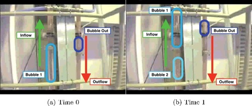
Figure 3. Screenshots from a movie showing a Pu-Nitrate surrogate solution moving through pipes similar to the PCDF equipment. Using the same type of pump system, bubbles can be seen intermixed with the solution in the pipes. Note that bubbles also exist in the outflow pipe and move upward toward the airlift separator. See online version for color.

While the background radiation from hold-up in the equipment was measurable, the radiation intensity of the solution was unknown. For detector capability and safety, the measurement was performed using a lanthanum-bromide (LaBr₃) detector that has higher rate capabilities and is more neutron-resistant compared to a standard high-purity germanium (HPGe) detector. A 5-cm-thick high-density polyethylene (HDPE) and 5-cm-thick lead (Pb) shield was placed below, above, and to the sides of the detector with only HDPE placed in front (see Figure 2(b)). This configuration reduced the effects of the background and overall rates while providing a measure of collimation that would not have been available otherwise. The data acquisition system (DAQ) and power supply were set on a separate cart with a fiber optic cable used to transfer the data to a computer in the low-radiation room next door.

The data was collected using a list-mode DAQ [16] to provide gamma-ray event energy and detection time with 10-ns resolution. The time stamp of the GRs enables operators and inspectors to determine the rate that particular nuclides are observed that can then be used to determine flow-rates or times of composition changes. Integrating over the entire transfer period, the GR energy spectrum can be used for composition analysis and compared to the random samples to verify process consistency. The energy limit was set to ∼11.9 MeV to enable observation of the natural background, neutron activation of the equipment, and any possible solution self-activation. Energy calibration measurements showed that there is a gain shift in this DAQ related to the count-rate of the GRs.

2.1. Pu-Nitrate sample

The NM details of the Pu-Nitrate solution used for this measurement are described in Table 1. Due to time restrictions, no high-resolution measurement was performed with an HPGe detector on a sample of the solution. However, it had a composition similar to another Pu-Nitrate sample, P135, that was measured with a HPGe detector for a different experiment [17] (see Table 1). Due to the lower resolution of the LaBr₃ detector compared to the HPGe detector, it was expected that the pipe-monitoring measurement would produce spectra with no significantly discernible GR peak differences between P136 and P135.

Table 1. Composition, density, and measurement days for the transferred Pu-Nitrate sample, P136, and a similar composition sample, P135

		P136	P135	Unit
Isotopic fractions	Pu-238	1.247	1.247	weight%
	Pu-239	56.989	56.966	weight%
	Pu-240	32.486	32.498	weight%
	Pu-241	3.175	3.182	weight%
	Pu-242	6.103	6.107	weight%
Pu concentration		136.6	160.9	g/L
Am-241 concentration		3.142	4.683	g/L
Density		1.373	1.411	g/cm^3
DA measurement day		6/6/2016	5/17/2016	m/d/y
Measurement day		6/14/2016	5/30/2016	m/d/y

2.2. Transfer process data and interpretation

Figure 4(a) shows the measured GR count rate using 1-s time bins overlaid on the change in volume of the SMMS-style electromanometer (EM) before (pre-), during, and after (post-) the transfer. To compare the data, time stamps for both the GR data and the EM data are given relative to the start of the GR collection time. Approximately 142 L of Pu-Nitrate solution was transferred from the input tank to the output tank during this measurement. The transfer begin and finish notice times were received at 1157 and 3017 s after starting collecting data (see Figure 4(a) and Table 2). The EM data around the beginning of the transfer was not recorded since the level of the solution was measured manually and it took ∼20 minutes for the system to restart in auto-collection mode.

Figure 4. (a) Change in volume of solution in the input tank (circles) and output tank (squares) during the transfer compared to the gamma-ray measurement at the glovebox pipe (gray line) in 1-s integration time bins relative to when the detector started collecting data. The missing electromanometer (EM) data points are due to temporarily stopping the automated computer for manual operation. (b) The beginning of the transferred solution gamma rays binned over 1-s and 100-ms integration periods. (c) The end of the transferred solution gamma rays binned over 1-s and 100-ms integration periods. In all images, the relevant times are indicated.

Table 2. The times that events occurred during the pipe-monitoring according to the lab notebook (Notes), the input tank (In) and output tank (Out) electromanometer (EM) data, and gamma-ray (GR) detector live-time. All times are in seconds referenced to the start of the detector data collection. The times with an asterisk (^*) are the values to be calculated in the process analysis (see Section 4.3)

	Label	Notes	EM	GR	Explanation
Beginning	^notesTb	1157	–	–	Notified transfer will begin
	^InTb	–	1249	^*	Solution begins flowing, input tank
	T^instart	–	–	1286	Solution first observed in inflow pipe
	T^outstart	–	–	1298	Solution first observed in outflow pipe
	^OutTb	–	1326	^*	Solution begins flowing, output tank
Ending	Tlast	–	-	2816	Solution finishes entering inflow pipe
	Tout	–	–	2827	Solution dominantly in outflow pipe
	T′end	–	–	2868	Last of solution enters outflow pipe
	Tend	–	–	2875	Last of solution leaves outflow pipe
	Tstop	–	–	2879	Return to hold-up plus activation rates
	^InTf	–	2884	^*	Solution finishes flowing, input tank
	^OutTf	–	2968	^*	Solution finishes flowing, output tank
	^notesTf	3017	–	–	Notified transfer finished

The nominal flow-rate of 0.0866 L/s was calculated by averaging the nominal linear fit results of the input and output tanks’ EM volume changes between the start and stop notice times. Using the individual flow-rates and pre- and post-transfer volumes, the true transfer beginning and finishing times were calculated (see Table 2). Since the EM data points are not truly linear, the times associated with the flow-rates are not as precise as the individual readings. It should be noted that there was a short delay between the beginning and finishing notices and the EM times, resulting in the notices as absolute time bounds.

The increase in GR counts above the hold-up background in Figure 4(b) indicates the time, Tⁱⁿ_start, that the solution in the inflow pipe was first observed by the detector (see Table 2). Changing the integration time bins of the list-mode data (e.g. 1 s compared to 100 ms) adjusts the details and precision during the transfer process without losing the accuracy in process event time interpretations. The GRs emitted from the solution follow the relative probability distribution along the transfer pipes as determined from an MCNP [18] model of the pipe structure (see Figure 5 a). Approximately 99% of the GRs observed from the inflow pipe are emitted from within an average sensitive region, Lⁱⁿ_GR, between zⁱⁿ_GR =[−5.9 (3), 91 (4)] cm, peaked at 15.9 cm.

Figure 5. (a) The MCNP-modeled relative probability distribution (left) and cumulative distribution function (CDF) (right) of the vertical height from which gamma rays generated along the inflow pipe and outflow pipe (indicated in the legend) can be observed by the detector referenced from the top of the concrete floor. The horizontal lines indicate vertical positions as described in the text. (b) A simulation depicting the gamma-ray integrated count as a 5-cm length of the solution passes through the sensitive region of the inflow pipe, similar to Figure 3. The time (left) is calculated using the EM flow-rate converted into linear speed (see Section 4.1). The variable size of the circles in the position plot (right) indicates the relative intensity of the counts in the detector.

The further increase at T^out_start in Figure 4(b) indicates that the solution was first observed within the outflow pipe, as justified by the count-rate difference at the end of the transfer between T_out and T_end of Figure 4(c). The average sensitive region of the outflow pipe, L^out_GR, falls between z^out_GR =[−4.8 (3), 101.3 (49)] cm, peaked at 19.4 cm. As expected, the detector first observes GRs halfway between the input tank and the output tank begin times.

The effects of the air bubbles pushing the solution through the pipes is observed as pulsing in the count-rate during the transfer starting just after T^out_start in Figure 4. Using 100-ms integration time bins, the low count-rates of Figure 4(b,c) indicate a bubble is dominantly observed in the inflow pipe with various amounts of solution observable in the outflow pipe. The count-rate spikes indicate that a short length of solution is passing through the inflow pipe in front of the detector, with the intensity and time-period being a convolution of the length of the solution and the position vertically along the pipe (see Figure 5(b)). Additionally, there is an underlying background that modulates the pulsing, producing a multi-modal frequency appearance that is suspected to be aliasing between the pulsing in the two pipes, though there was no way to physically observe the solution to verify this. This pulsing is only due to the method of homogenization used in the input tank (see Section 2) and would not appear for continuous-flow processes where paddles, etc. are used instead.

The final count-rate increase at T′_end of Figure 4(c) is suspected to be the observation of the last solution length in the outflow pipe which disappears from view at T_end, returning to the hold-up rate plus decaying neutron activation of the environment. However, all of the end-of-transfer process event times determined by the GR data occur before the input tank registers empty (see Table 2). Using the 37-s difference between Tⁱⁿ_start and ^InT_b, T_last should be at 2921 compared to ^InT_f, 105 seconds past the last measured peak. This extra time during the higher count-rate portion of the transfer accounts for ∼61% of the entire ∼173-s dead-time. Other experiments utilizing this system recorded data with the time-difference (lag) option and no deviations were observed (Makii H, personal communication). Since these event times are based on the DAQ live-time and are compressed relative to the tanks’ real-time values, it is suspected that the live-time varies according to the instantaneous count-rate, similar to the gain shift. However, this compression biases the timing terms in the process calculations of Section 4.

2.3. Gamma-ray count-rate filtering

Adapted from detector pulse-height analysis [19], the analysis performed here uses a filter that compares two integrated periods prior to each time bin, t_i: (1) $$\begin{array}{c}\hfill I_A\left(t_i\right)=\sum _{n=t_i-3}^{t_i-1}{\int }_{E}C(n,e_i)d{e}_i\end{array}$$(1) and (2) $$\begin{array}{c}\hfill I_B\left(t_i\right)=\sum _{n=t_i-6}^{t_i-4}{\int }_{E}C(n,e_i)d{e}_i\end{array}$$(2) where C(n, e_i) is the number of counts in the GR energy bin, e_i, detected for individual time bins, n (see Figure 6(a)). This not only increases the statistical measurement, it removes much of the randomness of the nominal count-rate. Using 0.5- to 0.1-s integration time-bins enhances the change in observable NM (e.g. the solution and air-bubble pulsing) observed by the detector (see Figure 6(b)) that can be used for high-precision time determination. This study uses 1-s integration periods to reduce the number of calculations, which, since there is a timing bias, emphasizes the aliasing with the outflow pipe (see Figure 6(c)) but improves the composition counting comparisons.

Figure 6. (a) An example of how I_A(t_i) (long dash) and I_B(t_i) (short dash) are determined from the data (solid) for a 1-s t_i time bin (filled gray). (b) The beginning of the transfer with 500-ms time bins clearly shows inflow solution pulsing following initial continuous flow before T^out_start. (c) The beginning of the transfer with 1-s integrations averages the inflow and outflow count-rates to produce aliased pulsing. The ϵ_F (dot-dash) indicates the trigger threshold level used to determine when there is a count-rate change.

Utilizing Poisson statistics, the event times and air-bubble-induced pulsing are calculated from I_A(t_i) and I_B(t_i) as (3) $$\begin{array}{c}\hfill F\left(t_i\right)=ln\left(\frac{I_A\left(t_i\right)}{I_B\left(t_i\right)}\right),\end{array}$$(3) where F(t_i) is given in fractional units. Mathematically, $$\begin{array}{c}\hfill F\{\begin{array}{cc}\hfill >0,& \hfill \mathrm{if}{I}_A>I_B\left(solution\right)\\ \hfill =0,& \hfill \mathrm{if}{I}_A=I_B\left(continuous\right)\\ \hfill <0,& \hfill \mathrm{if}{I}_A<I_B\left(bubble\right)\end{array}\end{array}$$where, beyond the indicated pulsing attributes, the first case would trigger when the solution first arrives to the detector, T_start, and the last case would trigger when the last of the solution becomes unobservable by the detector, T_stop. However, real detection must exceed a threshold above the effects of random counts, |ϵ_F|, usually around a 4σ excess (∼99.987% confidence), which produce periods of no clear solution or bubble pulsing.

3. Composition verification through gamma-ray spectral analysis

Figure 7 shows the low-energy GR-integrated count-rate spectrum of the P136 solution passing through the pipe (transfer) in comparison to the hold-up spectrum before and after the transfer (pre- and post-transfer) and the P135 spectrum. Due to the lower resolution of LaBr₃ and wide energy range used for this measurement, each observed peak is composed of one or more P135 GRs dominated by a primary nuclide: ²³⁸Pu, ²³⁹Pu, and ²³⁷U and ²⁴¹Am from ²⁴¹Pu α- and β-decay. Also implied by Figure 7, is that, if no deviations are detected, the integrated spectrum during the entire transition could potentially be used for composition analysis after the process concludes.

Figure 7. A comparison of the measured solution count rates per energy bin before (light gray), during (thick black), and after (dark gray) the transfer period in the 200- to 850-keV energy region. The P135 (dotted) spectrum measured statically with a HPGe in a different glovebox is arbitrarily scaled for comparison. The primary nuclide producing each gamma-ray peak is indicated for each prominent peak in the solution spectrum. The label ‘Ann.’ indicates the 511-keV annihilation peak.

From the safeguards perspective, GR pipe-monitoring would focus on verifying that the composition of the solution remains constant during the process. A single homogenized solution would emit a GR spectrum with the peak ratios unique to the composition and the rates unique to the quantity of NM visible by the detector. Safeguards would verify that the solution and process are consistent with declarations by monitoring for any significant differences in the GR spectrum that would indicate the composition or quantity changed. This spectral analysis focuses on establishing the capability to detect changes in NM composition or quantity.

3.1. Monitoring for composition change

Modifying Equation (1(1) $$\begin{array}{c}\hfill I_A\left(t_i\right)=\sum _{n=t_i-3}^{t_i-1}{\int }_{E}C(n,e_i)d{e}_i\end{array}$$(1) ), the count, C, of specific energy peaks, γ, can be determined for any time bin, t_i, by (4) $$\begin{array}{c}\hfill N_{\gamma }\left(t_i\right)=\sum _{n=t_i-3}^{t_i-1}{\int }_{\gamma -\delta }^{\gamma +\delta }C(n,e_i)d{e}_i,\end{array}$$(4) where the specific energy region, ±δ, is determined by the resolution of the detector and, as for this measurement, any energy-gain shifts. Figure 8 shows a few examples of N_γ(t_i) for each time bin during the entire measurement. While the NM GRs increase above the hold-up background during the transfer, the natural ¹³⁸La/⁴⁰K peak is largely unaffected by any external factors. The list of GRs can be pre-defined for any material within the facility depending the solution expected to be passing through the pipes (i.e. Pu-Nitrate, dissolved SNF).

Figure 8. A comparison of the 1-s integrated count-rate over the entire measurement time for the integrated spectrum (total) and indicated gamma-ray peaks. The gamma rays appearing from the Pu-Nitrate sample all have a clear rise during the transfer time. The natural peak, derived from ⁴⁰K (1462 keV) and ¹³⁸La (1438 keV), is largely unaffected by the sample transfer. Also indicated is the average background rate of the 208-keV region (dotted line) from hold-up in the equipment, and the transfer beginning and finishing notice times (dashed lines).

To verify that there is no change in composition, the ratios between the N_γ(t_i) should remain constant (within counting uncertainties) regardless of potential rate fluctuations. The ratio (5) $$\begin{array}{c}\hfill R_{\gamma }\left(t_i\right)=\frac{N_{\gamma }\left(t_i\right)}{N_{{\gamma }^{\text{'}}}\left(t_i\right)}\end{array}$$(5) specifically compares each peak, γ, to a reference peak, γ′. Able to be performed in real time, R_γ(t_i) should be within η_γ = 4 ×RMS of the mean for all time bins, t_i, during a process, with variability primarily driven by the pumping method. A change in the composition would be indicated by any GR peak appearing with |R_γ(t_i)| > η_γ, especially if this happens for more than one peak.

For this Pu-Nitrate solution, prominent spectral peaks are compared to the ²³⁹Pu 414-keV reference peak, N₄₁₅, for F(t_i) > ϵ_F (solution), F(t_i) < −ϵ_F (bubble), and the average (see Table 3). Figure 9 shows an example of N₆₅₈(t_i) and R₆₅₈(t_i) for the peak dominated by the 662-keV from ²⁴¹Am. While solution was in the inflow pipe, R₆₅₈ remained relatively stable within η₆₅₈, indicating that there was no deviation in the composition. During the only-outflow period (defined in Table 2), there is more attenuation of the 414-keV GR than the 662-keV GR by the GB structural support that results in R₆₅₈(t_i) ≳ η₆₅₈. Before and after the transfer, R₆₅₈ is at a different value, indicating that the hold-up background composition is different from the P136 solution. Comparatively, R₁₄₆₀ drastically changes between the three different pulsing types, though all within error of each other. Future experiments and deployment can reduce variability and improve detection by optimizing the location and shielding of the detector.

Table 3. The set of primary gamma-ray energy peaks observed during the transfer of Pu-Nitrate with the primary nuclide and calculated ratio R_γ for the period when solution is in the inflow pipe (see Table 2) for the three different pulsing possibilities defined for F (see Equation (3(3) $$\begin{array}{c}\hfill F\left(t_i\right)=ln\left(\frac{I_A\left(t_i\right)}{I_B\left(t_i\right)}\right),\end{array}$$(3) ) and Figure 6)

			Rγ = Nγ/N415 − keV
Emean	Primary	Erange	Mean (RMS)
(keV)	nuclide	[keV,keV]	Solution	Bubbles	${\bar{R}}_{\gamma }$
203	^237U	[190,220]	14.8 (8)	14.7 (8)	14.7 (8)
269	^237U	[255,285]	3.8 (2)	3.8 (2)	3.8 (2)
310	^239Pu	[295,325]	4.03 (20)	4.02 (19)	4.02 (19)
332	^241Am	[325,350]	2.5 (1)	2.4 (1)	2.4 (1)
373	^239Pu	[360,390]	1.67 (9)	1.67 (8)	1.67 (9)
415	^239Pu	[400,430]	1 (0)	1 (0)	1 (0)
658	^241Am	[635,680]	0.39 (4)	0.40 (4)	0.40 (4)
724	^241Am	[698,745]	0.25 (3)	0.26 (3)	0.25 (3)
767	^238Pu	[750,785]	0.14 (2)	0.14 (2)	0.14 (2)
1460	^40K/^138La	[1385,1525]	0.4 (1)	0.4 (1)	0.4 (1)
2208	^1H-act.	[2150,2270]	0.06 (2)	0.06 (2)	0.06 (2)
2609	^208Tl	[2530,2675]	0.05 (1)	0.05 (1)	0.05 (1)

Figure 9. Top: the 3-s integrated gamma-ray counts, N₆₅₈, between 635 and 680 keV (dominantly the ²⁴¹Am 662-keV gamma ray) for each time bin between the begin and finish notices. The gamma ray source types and event times noted in the legend are described in Section 2.2. ‘Other’ refers to no clear pulsing during the transfer and times outside of the transfer period. Bottom: the ratio, R₆₅₈, of the above gamma-ray peak counts compared to the peak counts dominated by the ²³⁹Pu 414-keV reference peak. While solution is in the inflow pipe, the ratio is within η₆₅₈ of the mean but increases when solution is only in the outflow pipe (T_last < t_i < T_end) before returning to the hold-up value. Relevant times are indicated.

3.2. Monitoring for malfunction or misuse

Changes in the solution spectrum may also arise from malfunction or other forms of misuse but would not necessarily change the composition peak–ratio differences. The composition analysis of Section 3.1 compares specific integrated GR peaks to verify that the GR ratios, and therefore composition, remain consistent. However, removing a small amount of Pu-Nitrate and replacing it with a Co-60 or Pb solution would change the Compton background and reduce the rates, but the Pu GR R_γ would remain constant. Analyzing the general shape of the spectrum for deviations allows inspectors to verify that the quantities are also consistent with declarations or if there is a problem in the process.

Removing the integral of Equation (4(4) $$\begin{array}{c}\hfill N_{\gamma }\left(t_i\right)=\sum _{n=t_i-3}^{t_i-1}{\int }_{\gamma -\delta }^{\gamma +\delta }C(n,e_i)d{e}_i,\end{array}$$(4) ), Equation (3(3) $$\begin{array}{c}\hfill F\left(t_i\right)=ln\left(\frac{I_A\left(t_i\right)}{I_B\left(t_i\right)}\right),\end{array}$$(3) ) can be rewritten to (6) $$\begin{array}{c}\hfill S_i=ln\left(\frac{C(t_i,e_i)}{C(t_{i-1},e_i)}\right)\end{array}$$(6) for the 3-s integrated counts, C, of each individual time, t_i, and energy, e_i, bin. For consecutive time bins, fitting S_i to a flat line (average), $\overline{\delta S}$, provides a continuous indication of the overall spectral shape deviation indicative of a solution change.

Figure 10(a) shows that the hold-up spectrum of C(1285) and C(1286) remains constant as indicated by the $\overline{\delta S}=-0.3\%$ of the 1286-s in Figure 10(b). Similar to R₆₅₈, the solution introduces a composition change from hold-up of $\overline{\delta S}=38.1\%$ at C(1287). Once the composition remains relatively consistent (e.g. C(1290) ≈ C(1289)), then $\overline{\delta S}$ returns to a relatively small difference.

Figure 10. The 3-s integrated count spectra, C(t_i, E) (a), and the difference between consecutive spectra, S_i (b), at the beginning of the transfer for the times indicated in the legends for the same energy region shown in Figure 7. See online version for color.

There are variations in the spectral shape caused by the pulsing due to the air bubbles suppressing the rate that the solution GRs are observed (see Figure 11), and a continuous stream would have less variation during the transfer. For the pre- and post-transfer hold-up, the compositions are stable and result in a mean variance of ${\sigma }_{\overline{\delta S}}^{holdup}=0.86\pm 0.06\%$. During this transfer, the mean variance is double-peaked: ${\sigma }_{\overline{\delta S}}^{stable}=1.8\pm 0.1\%$ for much of the time between 1480 and 1580 s; and ${\sigma }_{\overline{\delta S}}^{pulsed}=9.3\pm 1\%$ away from these times.

Figure 11. The composition difference, S_i, average spectral deviation between consecutive time bins for the period shown in Figure 9. The variations are all caused by differences between the solution gamma-ray spectral distribution and the hold-up gamma-ray spectral distribution with the solution arrival producing a significant spike at 1287 s as shown in Figure 10. The error bars are the uncertainty of fitting S_i to a flat line. Relevant times are indicated.

While it is difficult to quantify the sensitivity for this single measurement, further experiments with improved designs, high-resolution HPGe detectors, and secondary solutions introduced into the flow would improve the quality and qualification of this composition verification capability. However, both the peak-integration comparison method and the spectral-scale deviation method demonstrate the ability for GR pipe-monitoring to detect differences in real time indicative of an NM change.

4. Gamma-ray monitoring of the transfer process

Using the detector timing capabilities, radiation physics of the experimental setup, and physical characteristics of the process system, GR pipe-monitoring can determine the solution flow-rate which directly affects the evaluation of the total volume of the solution that passes through the pipes and the process time period. While the solution process event times for this measurement have a live-time bias (see Section 2.2), the calculations performed here are correct in concept and approach. Future measurements that account for the dead-time properly will improve the accuracy, precision, and veracity of this process evaluation.

4.1. Evaluating the solution flow-rate

Associating the last pulse in the outflow count-rate in Figure 4(c) as the last of the solution passing L^out_GR, the outflow linear speed can be estimated as (7) $$\begin{array}{c}\hfill v_{lin}^{out}=\frac{L_{GR}^{out}}{\delta T_{end}}=\frac{{|}_{low}{z}_{GR}^{out}{-}_{high}{z}_{GR}^{out}|}{T_{end}-T_{end}^{\text{'}}},\end{array}$$(7) where T′_end and T_end are from Table 2 and L^out_GR is defined in Section 2.2 in association with Figure 5. The pulsing would not be observed with a continuous-flow transition, which would require a different method of determining v^out_lin.

Table 4 shows the values calculated from the GR data and the comparison with the EM data values. The average linear speed for the input (In) and output (Out) tanks is determined as (8) $$\begin{array}{c}\hfill {}^{In,Out}{v}_{lin}=\frac{{}^{In,Out}V}{\left({\Delta }^{In,Out}T\right)A^{in,out}},\end{array}$$(8) where V is the volume difference shown in Figure 4(a) (see Table 4), ΔT = T_f − T_b is the calculated transfer time derived from Table 2, and Aⁱⁿ = 3.597 (2) cm² and A^out = 6.158 (2) cm² are the cross-sectional areas of the inflow and outflow pipes. The accuracy and precision for all values calculated in this process analysis, X, is determined by (9) $$\begin{array}{c}\hfill \Delta X{=}^{GR}X{-}^{EM}X\end{array}$$(9) with an error of (10) $$\begin{array}{c}\hfill {\sigma }_{\Delta X}=\sqrt{{\left({\sigma }_{{}^{GR}X}\right)}^2+{\left({\sigma }_{{}^{EM}X}\right)}^2},\end{array}$$(10) where GR are the analysis values determined here and EM are the noted input (In) and output (Out) tank times. The v^out_lin calculated from the GR data is ∼8% greater than the input tank EM speed, which correlates to the live-time bias.

Table 4. Comparisons of values calculated from the gamma ray (GR) data and compared to the fits from the electromanometer (EM) data for the linear velocity (v_lin), volumetric flow-rates (R_V), and total volume transferred (V) through the inflow (in) and outflow (out) pipes. The inflow terms are calculated using the using Equations (13(13) $$\begin{array}{c}\hfill v_{lin}^{in}=\frac{L^{in}}{T_{start}^{out}-T_{start}^{in}-\frac{L^{out}}{v_{lin}^{out}}}\end{array}$$(13) ) and (14(14) $$\begin{array}{c}\hfill v_{lin}^{in}=\frac{L_{GB}{-}_{low}{z}_{GR}^{in}{-}_{high}{z}_{GR}^{out}}{T_{start}^{out}-T_{start}^{in}},\end{array}$$(14) ) as indicated. The v_lin and R_V are compared between the input (In) and output (Out) tank EM data calculated values (ΔX) with V compared to the average (bold). The values in parentheses are the uncertainty on the calculated last digit

Value	EM			GR	ΔX	Eq. #
vlin (cm/s)		In	24.2 (2)	27.0 (47)	2.8 (47)	(13(13) $$\begin{array}{c}\hfill v_{lin}^{in}=\frac{L^{in}}{T_{start}^{out}-T_{start}^{in}-\frac{L^{out}}{v_{lin}^{out}}}\end{array}$$(13) )
				26.7 (31)	2.5 (31)	(14(14) $$\begin{array}{c}\hfill v_{lin}^{in}=\frac{L_{GB}{-}_{low}{z}_{GR}^{in}{-}_{high}{z}_{GR}^{out}}{T_{start}^{out}-T_{start}^{in}},\end{array}$$(14) )
		Out	14.03 (9)	15.1 (17)	1.1 (17)	(7(7) $$\begin{array}{c}\hfill v_{lin}^{out}=\frac{L_{GR}^{out}}{\delta T_{end}}=\frac{{|}_{low}{z}_{GR}^{out}{-}_{high}{z}_{GR}^{out}|}{T_{end}-T_{end}^{\text{'}}},\end{array}$$(7) )
RV (mL/s)	86.6 (9)	In	87.0 (7)	97.1 (167)	10.1 (167)	(13(13) $$\begin{array}{c}\hfill v_{lin}^{in}=\frac{L^{in}}{T_{start}^{out}-T_{start}^{in}-\frac{L^{out}}{v_{lin}^{out}}}\end{array}$$(13) )
				96.0 (112)	9.0 (112)	(14(14) $$\begin{array}{c}\hfill v_{lin}^{in}=\frac{L_{GB}{-}_{low}{z}_{GR}^{in}{-}_{high}{z}_{GR}^{out}}{T_{start}^{out}-T_{start}^{in}},\end{array}$$(14) )
		Out	86.4 (5)	93.2 (103)	6.8 (103)	(7(7) $$\begin{array}{c}\hfill v_{lin}^{out}=\frac{L_{GR}^{out}}{\delta T_{end}}=\frac{{|}_{low}{z}_{GR}^{out}{-}_{high}{z}_{GR}^{out}|}{T_{end}-T_{end}^{\text{'}}},\end{array}$$(7) )
V (L)	141.7 (57)	In	142.2 (56)	148.5 (256)	6.3 (256)	(13(13) $$\begin{array}{c}\hfill v_{lin}^{in}=\frac{L^{in}}{T_{start}^{out}-T_{start}^{in}-\frac{L^{out}}{v_{lin}^{out}}}\end{array}$$(13) )
				146.8 (172)	4.6 (172)	(14(14) $$\begin{array}{c}\hfill v_{lin}^{in}=\frac{L_{GB}{-}_{low}{z}_{GR}^{in}{-}_{high}{z}_{GR}^{out}}{T_{start}^{out}-T_{start}^{in}},\end{array}$$(14) )
		Out	141.8 (10)	146.3 (162)	4.2 (162)	(7(7) $$\begin{array}{c}\hfill v_{lin}^{out}=\frac{L_{GR}^{out}}{\delta T_{end}}=\frac{{|}_{low}{z}_{GR}^{out}{-}_{high}{z}_{GR}^{out}|}{T_{end}-T_{end}^{\text{'}}},\end{array}$$(7) )

As described in Section 2.2, Tⁱⁿ_start determines the time that the detector first observes the solution arriving to _lowzⁱⁿ_GR in the inflow pipe position and T^out_start correlates to approximately the high position of the outflow pipe, _highz^out_GR (see Figure 4(b)). The length of the pipes in the GB is composed of two terms (11) $$\begin{array}{c}\hfill L_{GB}=l^{in}+l^{out},\end{array}$$(11) where lⁱⁿ = 225.9 (2) cm is the inflow pipe above the concrete floor where the solution is pulled by the air-lift pump, l^out is the outflow pipe above the concrete floor and the air-lift separator tank length where the solution is pulled by gravity, and L_GB = 420.9 (3) cm. The time it takes to travel between these positions with potentially different flow rates is determined by (12) $$\begin{array}{ccc}\hfill T_{start}^{out}-T_{start}^{in}& =& \frac{L^{in}}{v_{lin}^{in}}+\frac{L^{out}}{v_{lin}^{out}}\hfill \\ & =& \frac{l^{in}{-}_{low}{z}_{GR}^{in}}{v_{lin}^{in}}+\frac{\left(l^{out}{-}_{high}{z}_{GR}^{out}\right)\left(\frac{A^{in}}{A^{out}}\right)}{v_{lin}^{out}},\hfill \end{array}$$(12) where the A ratio arises since the head of the solution does not increase to the area of the outflow pipe until the solution builds up in the pipe further into the transfer, as viewed in the movie used to derive Figure 3 (not shown). Solving Equation (12(12) $$\begin{array}{ccc}\hfill T_{start}^{out}-T_{start}^{in}& =& \frac{L^{in}}{v_{lin}^{in}}+\frac{L^{out}}{v_{lin}^{out}}\hfill \\ & =& \frac{l^{in}{-}_{low}{z}_{GR}^{in}}{v_{lin}^{in}}+\frac{\left(l^{out}{-}_{high}{z}_{GR}^{out}\right)\left(\frac{A^{in}}{A^{out}}\right)}{v_{lin}^{out}},\hfill \end{array}$$(12) ) for the inflow pipe flow rate (13) $$\begin{array}{c}\hfill v_{lin}^{in}=\frac{L^{in}}{T_{start}^{out}-T_{start}^{in}-\frac{L^{out}}{v_{lin}^{out}}}\end{array}$$(13) results in a ∼10% greater speed attributed to the timing bias, as shown in Table 4.

Alternatively, the inflow linear velocity can be calculated by just taking the length difference between the L_GR terms as (14) $$\begin{array}{c}\hfill v_{lin}^{in}=\frac{L_{GB}{-}_{low}{z}_{GR}^{in}{-}_{high}{z}_{GR}^{out}}{T_{start}^{out}-T_{start}^{in}},\end{array}$$(14) where the value is essentially the same value as the full calculation (see Table 12(12) $$\begin{array}{ccc}\hfill T_{start}^{out}-T_{start}^{in}& =& \frac{L^{in}}{v_{lin}^{in}}+\frac{L^{out}}{v_{lin}^{out}}\hfill \\ & =& \frac{l^{in}{-}_{low}{z}_{GR}^{in}}{v_{lin}^{in}}+\frac{\left(l^{out}{-}_{high}{z}_{GR}^{out}\right)\left(\frac{A^{in}}{A^{out}}\right)}{v_{lin}^{out}},\hfill \end{array}$$(12) ). This confirms that the A ratio in Equation (12(12) $$\begin{array}{ccc}\hfill T_{start}^{out}-T_{start}^{in}& =& \frac{L^{in}}{v_{lin}^{in}}+\frac{L^{out}}{v_{lin}^{out}}\hfill \\ & =& \frac{l^{in}{-}_{low}{z}_{GR}^{in}}{v_{lin}^{in}}+\frac{\left(l^{out}{-}_{high}{z}_{GR}^{out}\right)\left(\frac{A^{in}}{A^{out}}\right)}{v_{lin}^{out}},\hfill \end{array}$$(12) ) indicates that the head of the solution remains ∼Aⁱⁿ for this calculation, though using 97. Consequently, this verifies that Equation (13(13) $$\begin{array}{c}\hfill v_{lin}^{in}=\frac{L^{in}}{T_{start}^{out}-T_{start}^{in}-\frac{L^{out}}{v_{lin}^{out}}}\end{array}$$(13) ) is not required if v^out_lin cannot be determined, as for a continuous-flow transition, but can be inverted to determine v^out_lin if appropriate time differences are observed.

The flow-rates (15) $$\begin{array}{c}\hfill R_V^{in,out}=v_{lin}^{in,out}{A}^{in,out}\end{array}$$(15) are initially dominated by vⁱⁿ_lin. Calculating R^{in, out} determines the input and output tank volume-change flow-rate to within the ∼9% bias in v_lin (see Table 4).

Using narrower collimation to reduce the L_GR and the excessive count-rates that introduce the timing bias can improve the flow-rate accuracy and precision. Alternatively, placing two detectors along a single process pipe at a fixed, known distance and measuring the time difference between the two T_start values would provide very accurate and precise values. Regardless, the calculations show that GR pipe-monitoring can determine the flow-rate of solution within the pipes using a single detector.

4.2. Estimating total solution volume transferred

The volumes determined from the EM data are derived from the difference of the mean weight before and after the transfer (see Table 4). The uncertainty is evaluated based on the root-mean-square of the average variance in the mean values during these stable periods, similar to Burr [7]. Burr showed a relative change for stable (wait) periods of ∼4% that are similar to the fractional variation of the input tank, primarily from when it was empty after the transfer.

Using the flow-rates determined in Section 4.1, the volume of the solution passing the detector is estimated as (16) $$\begin{array}{c}\hfill {}^{In,Out}V=R_V^{in,out}{T}_{Live}^{in,out},\end{array}$$(16) where T_Live is the time difference between the arrival triggers of the first and last solution length from Table 2. Specifically, $$\begin{array}{c}\hfill T_{Live}=\{\begin{array}{cc}\hfill T_{last}-T_{start}^{in},& \hfill inflow\\ \hfill T_{end}^{\text{'}}-T_{start}^{out},& \hfill outflow\end{array}\end{array}$$results in the volumes given in Table 4. The live-time bias that affects both T_Live and the time differences used to calculate v_lin cancel out, resulting in values ≲ 3% in excess of the average of the EM data and well within the ∼11% uncertainties. This confirms the capability that GR pipe-monitoring can verify the volume of the solution passing by the detector.

4.3. Evaluating solution transition declared periods

The process beginning and finishing times, T_b and T_f, can be estimated from the linear speeds calculated from the GR data in Section 4.1 as (17) $$\begin{array}{c}\hfill {}^{GR}{T}_{b,f}{=}^{GR}{T}_{start,stop}+\frac{{}^{In,Out}L}{v_{lin}^{in,out}}\widehat{z},\end{array}$$(17) where ^{In, Out}L are the lengths of the inflow or outflow pipes below the concrete floor to the input and output tanks and the $\widehat{z}$ vector is in the direction of the solution flow. Table 5 shows T_b and T_f for this solution transfer calculated from both the GR data and from the fits to the EM data relative to the start of the measurement. As with the flow-rate, the accuracy and precision is determined by Equations (9(9) $$\begin{array}{c}\hfill \Delta X{=}^{GR}X{-}^{EM}X\end{array}$$(9) ) and (10(10) $$\begin{array}{c}\hfill {\sigma }_{\Delta X}=\sqrt{{\left({\sigma }_{{}^{GR}X}\right)}^2+{\left({\sigma }_{{}^{EM}X}\right)}^2},\end{array}$$(10) ) with the comparison focusing on the input tank begin time, ^InT_b, and the output tank finish time, ^OutT_f, since these are the true begin and finish times. Similar to the volume calculation from Section 4.2, the timing bias factors out of this equation since the observed T_{start, stop} are condensed, but the times in the denominator of v_lin are extended. As such, the values are within the quadrature error of the difference and GR pipe-monitoring conclusively demonstrates a capability to determine a process period, either declared or undeclared.

Table 5. Solution transfer begin (b) and finish (f) times calculated from the input (In) and output (Out) tank electromanometer (EM) data and gamma-ray (GR) data. The GR values were calculated from the solution linear speed, v_lin, shown in Table 4 for the pipe leading to the appropriate tank. The comparisons made between ^InT_b or ^OutT_f and the GR values (bold) define the true bounds of the transfer. All times are in seconds referenced to the start of the GR data collection. The values in parentheses are the uncertainty on the calculated last digit

Explanation	EM (s)		GR (s)	ΔT (s)	Eq. #
Solution flow begins	^InTb	1249 (39)	1257 (5)	8 (40)	(13(13) $$\begin{array}{c}\hfill v_{lin}^{in}=\frac{L^{in}}{T_{start}^{out}-T_{start}^{in}-\frac{L^{out}}{v_{lin}^{out}}}\end{array}$$(13) )
			1257 (2)	8 (39)	(14(14) $$\begin{array}{c}\hfill v_{lin}^{in}=\frac{L_{GB}{-}_{low}{z}_{GR}^{in}{-}_{high}{z}_{GR}^{out}}{T_{start}^{out}-T_{start}^{in}},\end{array}$$(14) )
	^OutTb	1326 (31)	1351 (7)	−28 (32)	(7(7) $$\begin{array}{c}\hfill v_{lin}^{out}=\frac{L_{GR}^{out}}{\delta T_{end}}=\frac{{|}_{low}{z}_{GR}^{out}{-}_{high}{z}_{GR}^{out}|}{T_{end}-T_{end}^{\text{'}}},\end{array}$$(7) )
Solution flow finishes	^InTf	2884 (39)	2846 (5)	−38 (40)	(13(13) $$\begin{array}{c}\hfill v_{lin}^{in}=\frac{L^{in}}{T_{start}^{out}-T_{start}^{in}-\frac{L^{out}}{v_{lin}^{out}}}\end{array}$$(13) )
			2846 (2)	−38 (39)	(14(14) $$\begin{array}{c}\hfill v_{lin}^{in}=\frac{L_{GB}{-}_{low}{z}_{GR}^{in}{-}_{high}{z}_{GR}^{out}}{T_{start}^{out}-T_{start}^{in}},\end{array}$$(14) )
	^OutTf	2968 (31)	2940 (7)	−28 (32)	(7(7) $$\begin{array}{c}\hfill v_{lin}^{out}=\frac{L_{GR}^{out}}{\delta T_{end}}=\frac{{|}_{low}{z}_{GR}^{out}{-}_{high}{z}_{GR}^{out}|}{T_{end}-T_{end}^{\text{'}}},\end{array}$$(7) )

5. Discussion and future work

The work by Burr is focused on solution tank monitoring addressing the ability to detect diversion of 1 significant quantity of SNM per year [6,7]. Following Burr and using the average EM volume uncertainty and false-positive and false-negative rates of β = 0.05 and α = 0.05, the standard detection limit [20] for a well-known blank (e.g. calibrated tank monitoring) would result in L^{EM − ave}_d = 18.8 liters, ∼13.3% of the average volume transferred (see Table 4). However, using only the output tank that was never empty, the variance of ∼0.7% provides a detection limit of L^{EM − out}_d = 3.25 liters, ∼2.3% similar to Burr. The relative difference between the GR-determined solution volume and the output-tank detection limit, though, is only ∼1.4σ, which is well within the average limit. Consequently, this indicates that there could be large systematic biases caused by empty tanks in the solution monitoring process, but the GR pipe-monitoring is rather accurate.

This GR pipe-monitoring technique, however, was designed to search for deviations from the expected by using detection capabilities similar to the triggering of particles within a detector voltage pulse stream [19]. For a continuous, non-pulsing stream similar to the hold-up background variance, Burr's 3σ deviation [6] indicates that this analysis has a detection limit of L^holdup_d ≈ 2.8% to observe deviations in the spectral shape for verification of the solution process. While this GR detection value is much higher than Burr's σ_{s, r} = 0.1% level, it is both consistent with the L^{EM − out}_d and able to monitor the NM directly. The observed solution transfer start, ${\overline{\delta S}}_{1287}=38.1\%$, is ∼13.5σ above the detection limit, with even the stable periods (∼${\overline{\delta S}}_{1290}$) ∼2σ above the hold-up detection limit. The challenge comes during the transfer period itself where the detection limit changes from ∼6% in the stable-flow regions to ∼30.5% in the pulsing regions. Though the solution transfer onset ${\overline{\delta S}}_{1287}$ exceeds the pulsed period detection limit, more measurements of solutions with different compositions and changes in those solutions would further develop the sensitivity threshold for this analysis.

Finally, from Table 3 , it can be seen that the average L^peaks_d ≈ 16% for the energies near 415 keV and gets worse while generally following an efficiency curve. Estimating that this provides the ability to determine that a composition remains constant, low-resolution detectors like LaBr₃ become a limiting factor to gamma-ray pipe monitoring. Using a nominal 0.3% resolution of high-purity germanium, the quadrature difference for a pair of peaks could produce L^HPGe_d ≈ 1.3% to ensure that the solution remains constant. How this would degrade with air-bubble pulsing is unclear but can only increase the value, again potentially similar to L^{EM − out}_d.

The analysis presented here demonstrates that measuring GRs generated by NM solution flowing through pipes effectively improves real-time monitoring capabilities by being able to

• verify NM composition consistency and observe deviations in the GRs indicative of a change in composition;

• associate the flow-rates, volume, and time period of the declared solution process; and

• detect deviations in the operational process and during declared periods of inactivity due to either equipment malfunction or misuse.

Though mass cannot be directly measured, GR pipe-monitoring is intended to support the SMMS system and improve monitoring capabilities between the key measurement locations. While there are differences and timing biases due to the DAQ used for this single measurement, additional experiments and simulations using different facilities, detectors, and solutions (e.g. single composition, introducing surrogates, complex SNF) will confirm the veracity of these results. Particular emphasis should be placed on evaluating timing corrections and output frequency (e.g. continuous list-mode or periodic measurement).

If no deviations are detected, the average of the pre- and post-transfer spectra can be subtracted from the transfer spectrum for high-statistics composition analysis. This can then be compared to input and output tank spectra to verify that there are no differences or potentially provide NDA isotopic composition analysis in lieu of batch sampling. Additionally, using continuous GR pipe-monitoring provides a method to evaluate hold-up increases over time from data collected during the non-transition periods.

Since this technique requires only one GR detector along the pipes between the solution tanks, the cost for each facility can be minimized through effective design. However, using two detectors would ensure an independent flow-rate evaluation, especially on unidirectional pipes. Additionally, compared to this experiment, high-rate HPGe detectors would perform better for spectral analysis [19] and electronically cooled detectors would be less dependent upon operator maintenance. Effective design can also reduce cross-signals in multi-process path environments since low-energy gamma rays from direct decay of the NM of interest can be easily shielded. Further evaluation is required to determine the lifetime of the individual detector and the frequency of replacement.

The methods demonstrated here were developed to be easily implemented on (or modified for) a fast analog-to-digital chip (FADC). As such, GR pipe-monitoring is an effective PM capability that can be performed from an unattended, in-line system in real time with remote/unattended operations enabled through appropriate technological equipment. Similar to SMMS, the data output can potentially be split for use by both inspectors and operators concurrently, providing facility-specific operational information to the operators while automated triggers could indicate abnormal operations to safeguards inspectors. Consequently, GR pipe-monitoring could enable inspectors to monitor all declared and undeclared activities while performing real-time safeguards verification.

6. Summary and conclusions

Using a list-mode DAQ to provide both event energy and time, we measured the GRs from a Pu-Nitrate solution flowing through transfer pipes at the JAEA PCDF. We developed a simple analysis for this single pipe-monitoring measurement that demonstrates the ability for gamma-ray pipe-monitoring to determine consistency of the composition, volume, flow-rate, and process period in real time for NM solution transitions. Consequently, this demonstrates that remote, online, in-line process monitoring is feasible to maintain real-time continuity-of-knowledge of all nuclear materials flowing through pipes, away from accountancy tanks. Able to monitor for deviations from the expected or unexpected processes further enables inspectors to detect misuse or malfunction, essential for the future of safeguards verification in nuclear reprocessing facilities. As such, gamma-ray pipe-monitoring provides a viable option to reduce the time and cost burdens of current safeguards verification and operational quantification.

Acknowledgments

This work is supported by the Ministry of Education, Culture, Sports, Science, and Technology (MEXT), Japan. We would also like to thank H. Makii from JAEA's Sector of Nuclear Science Research for lending us the list-mode data acquisition system.

Disclosure statement

No potential conflict of interest was reported by the authors.

Additional information

Funding

This work is supported by the Ministry of Education, Culture, Sports, Science, and Technology (MEXT), Japan.

References

- Reilly D, Ensslin N, Smith H Jr. et al, . Passive nondestructive assay of nuclear materials. Los Alamos, NM: Los Alamos National Laboratory; 1991. p. 278. ( Report no. LA-UR-90-732).
- Menlove HO, Holbrooks OR, Ramalho A. Inventory sample coincidence counter manual. Los Alamos, NM: Los Alamos National Laboratory; 1982. ( Report no. LA-9544-M).
- Ehinger MH, Zack NR, Hakkila EA, et al. Use of process monitoring for verifying facility design for large-scale reprocessing plants. Oak Ridge, TN: Oak Ridge National Laboratory; 1991. ( Report no. LA-12149-MS).
- Johnson SJ, Abedin-Zadeh R, Pearsall C, et al. Development of the safeguards approach for the Rokkasho Reprocessing Plant. IAEA SM. 2001;367(8):01.
- Garcia HE, Burr TL, Coles GA, et al. Integration of facility modeling capabilities for nuclear nonproliferation analysis. Progr Nucl Energy. 2012;54(1):96–111.
- Burr TL, Coulter CA, Howell J, et al. Solution monitoring: quantitative and qualitative benefits to nuclear safeguards. J Nucl Sci Technol. 2003;40(4):256–263.
- Burr T, Hamada MS, Howell J, et al. Estimating alarm thresholds for process monitoring data under different assumptions about the data generating mechanism. Sci Technol Nucl Install. 2013; Article ID 705878.
- Orton CR, Fraga CG, Christensen RN, et al. Proof of concept simulations of the multi-isotope process monitor: an online, nondestructive, near-real-time safeguards monitor for nuclear fuel reprocessing facilities. Nucl Instrum Methods Phys Res A. 2011;629(1):209–219.
- Orton CR, Fraga CG, Christensen RN, et al. Proof of concept experiments of the multi-isotope process monitor: an online, nondestructive, near real-time monitor for spent nuclear fuel reprocessing facilities. Nucl Instrum Methods Phys Res A. 2012;672:38–45.
- Meier DE, Coble JB, McDonald LW et al, . The Multi-Isotope Process (MIP) Monitor Project: FY13 final report. Richland, WA: Pacific Northwest National Laboratory; 2013. ( Report no. PNNL-22799).
- Goddard B. Development of a real-time detection strategy for material accountancy and process monitoring during nuclear fuel reprocessing using the Urex+3A method [master's thesis]. College Station: Texas A&M University; 2009.
- Meier D, Sexton L, Coble J et al, . Multi-isotope process (MIP) monitor deployment at H-Canyon. Proceedings. GLOBAL 2015; 2015 Sept 20–24; Paris, France.
- Gilliam N, Coble J, Meier D. Preprocessing analysis of the multi isotope process monitor. Trans Am Nucl Soc. 2017;116:334–337.
- Rodriguez DC, Koizumi M, Nakamura H et al, . Development of active neutron NDA techniques for non-proliferation and nuclear security. 5. Systematic uncertainty and preliminary fission yields from DGS measurements using an Inverse Monte Carlo analysis. Proceedings of INMM 57th Annual Meeting; 2016 July 24–28; Atlanta, USA [ Online].
- Brun R, Rademakers F. ROOT - an object oriented data analysis framework. Nucl Inst Methods Phys Res A. 1997;389:81–86.
- Yamada M, Saito J. 16-Input PHA & LIST module A3100. Niki Glass product manual [cited Nov. 2016]. Available from: http://www.nikiglass.co. jp/products/radiation/A3100_NIKI(R1)1.pdf
- Mukai Y, Ogawa T, Nakamura H et al, . Development of active neutron NDA techniques for nuclear nonproliferation and nuclear security (7): measurement of DG from MOX and Pu liquid samples for quantification and monitor of NM. Proceedings of INMM 57th Annual Meeting; 2016 July 24–28; Atlanta, USA. [ Online].
- Goorley T, James M, Booth T, et al. Initial MCNP6 release overview. Nucl Technol. 2012;180:298–315.
- VanDevender BA, Dion MP, Fast JE, et al. High-purity germanium spectroscopy at rates in excess of 106 events/s. IEEE Trans Nucl Sci. 2014;61(5):2619–2627.
- Currie LA. Limits for qualitative detection and quantitative determination: application to radiochemistry. Anal Chem. 1968;40(3):586–593.