An applied limit of the bunching method for the Feynman-α analysis

ABSTRACT

Feynman-α method is used as the representative method in reactor noise analysis for the criticality monitoring. Feynman-α analysis needs a large amount of measurement time in its original process, though many researchers use the bunching method and its derived methods for the experimental data processing to shorten the measurement time. However, the detailed characteristics and the application limit of the bunching method have not been researched and discussed enough. This paper shows a possibility that the Bunching method is a method to reduce the probability fluctuation with the Y value only in the appearance. Moreover, the criteria for determining that the Y value is not an accidental product are also provided in this paper.

KEYWORDS:

• Reactor noise
• Feynman-α
• bunching method
• applied limit
• error
• confidence interval
• computer simulation

1. Introduction

In mid 1950s, Feynman R. P. proposed an original technique to determine the prompt-neutron decay constant αα from a dispersion of the neutron emission in U-235 fission [1]. Later, this stochastic method has been referred to as ‘Feynman-α method.’ The experimental acquisition was repeated many times with changing the gate width to obtain a gate-width dependence of a statistical indication Y, which was defined as the variance-to-mean ratio of the neutron counts minus 1. Therefore, the Y values of various gate widths were statistically independent of each other.

In the recent Feynman-α experiments, however, time-sequence counts data within a specified gate width (e.g. 1 ms for a thermal critical system) were continuously registered by a multi-channel scaler (MCS), and the longer gate widths data (e.g. 2, 3, 4,…, 100 ms) are synthesized from the recorded MCS data. This synthesizing technique is generally called ‘bunching method’ [2]. Using the time-sequence count data generated by the synthesis, the Y was calculated in the longer gate-width range. An alternative bunching-technique referred to as ‘moving-bunching technique’ was also proposed to reduce the statistical scatter of the Y [3] with useful to reduce a time required for the experiment, i.e. to reduce a machine time. However, the technique uses the counts of a MCS channel multiple times to synthesize time-sequence counts within longer time widths. Therefore, the Y values of various gate widths were not statistically independent of each other. The statistical influence of the multiple uses on the Y value has been hardly investigated. In this way, the bunching technique has no theory for some justification and now it is an essential problem of this technique.

In spite of the above problem, the bunching technique has been successfully applied to determine the decay constant of various nuclear systems. However, in the case of that a neutron counter is placed far from a nuclear fuel region or an analyzed nuclear system has a large subcritical reactivity, the bunching technique leads to various strange and nonphysical behaviors of the Y. For an example, the Y value monotonically increases, decreases, oscillates, and so on with the prolonging in the gate width as found in reference [3]. For another difficult example, the technique results in a plausible gate-width dependence of the Y but only a nonphysical decay constant can be obtained from the Y value distribution. When we repeated acquiring time-sequence counts data within each gate width without the use of the bunching technique, most of the above nonphysical behaviors disappeared but only the scatter of the Y around zero appeared. These features have been observed in various challenging experiments with the much smaller Y than one and worried us for a long time.

Also, the Feynman-α method is attracting a great deal of attention in the field of a criticality monitoring for decommissioning and extracting fuel debris in the Fukushima Daiichi nuclear power station [4–6]. Because of the peripherals’ installing intractableness, the stochastic method can gbecome one of the applied measuring methods under various severe conditions, such as an extremely low efficiency of neutron detection for total fissions, a very large subcritical reactivity, a limited measurement time, and so on. Under these severe conditions, an application of the bunching technique will undoubtedly lead to a worrisome and nonphysical behavior of the Y, mentioned above. From the viewpoint of the criticality safety in the Fukushima-Daiichi decommission, the peculiar characteristics of the bunching technique and the application limits under the severe conditions are very important subjects to be clarified. However, these subjects have been hardly studied up to the present.

In this study, first, the influence of bunching technique on signal events obtained on the basis of the Poisson distribution (named ‘Poisson Events’ in this paper) is examined. For this purpose, the time-sequence counts data within a gate width are numerically generated based on the Poisson distribution and then the generation is many times repeated changing the gate width without using the bunching technique, to obtain the Y of the various gate widths. Subsequently, time-sequence counts data within only a gate width are numerically generated and then the Y values of the various gate widths are calculated from the time-sequence data synthesized by the bunching technique. The above two kinds of the Y are compared with each other to examine the characteristics and the application limit of the bunching technique. Further, the influence of the bunching technique on the non-Poisson, i.e. multiplicative events, is also examined from a comparison of the gate-width dependence of the Y obtained by the bunching technique with that obtained by a repeated generation of time-sequence data. In this paper, a theory of generating the time-sequence data based on the Poisson events and on the multiplicative events is described in Section 2, the discussion of the results in Section 3, and the conclusion of this study in Section 4.

2. Method and analysis

Simulated time series data are used to researches for the characteristics of the bunching method in this paper. Generating of Poisson events’ time series, generating of multiplication time series, analysis methods for the generated data, and criteria for determining analysis results are shown in the following.

2.1 Generation of time series Poisson events

A probability of time interval for Poisson events is expressed as follows [7]:

(1) $P\left(t\right)=exp\left(-r\cdot t\right)$(1)

where r [cps] is an average event rate in the unit time.

The time interval of ith event and i + 1th event, T_interval [i], is written with a uniform random number, Rand, as follows [8]:

(2) $T_{interval}\left[i\right]=-\frac{1}{r}\times log\left(Rand\right)$(2)

From this, an event time of nth event, T_event [n], is written as follows:

(3) $T_{event}\left[n\right]=\sum _n^{i=1}{T}_{interval}\left[i\right]$(3)

2.2 Generation of time series multiplication events

The reactor noise analysis is based on a distortion analysis of the time series data from the Poisson distribution. Multiple events are simulated by the following method using time series data generated in Section 3.1. First, nth event, generated in Section 3.1, is judged to be a seed of multiplication using a multiplication probability, p_multiple, and a uniform random number:

$\begin{array}{rl}& \mathrm{i}\mathrm{n}\mathrm{t}\mathrm{h}\mathrm{e}\mathrm{c}\mathrm{a}\mathrm{s}\mathrm{e}\mathrm{o}\mathrm{f}Rand\le p_{multiple}:\mathrm{G}\mathrm{e}\mathrm{n}\mathrm{e}\mathrm{r}\mathrm{a}\mathrm{t}\mathrm{e}\mathrm{M}\mathrm{u}\mathrm{l}\mathrm{t}\mathrm{i}\mathrm{p}\mathrm{l}\mathrm{e}\mathrm{d}\\ & \mathrm{E}\mathrm{v}\mathrm{e}\mathrm{n}\mathrm{t}\\ & \mathrm{i}\mathrm{n}\mathrm{t}\mathrm{h}\mathrm{e}\mathrm{c}\mathrm{a}\mathrm{s}\mathrm{e}\mathrm{o}\mathrm{f}Rand>p_{multiple}:\mathrm{n}\mathrm{o}\mathrm{t}\mathrm{G}\mathrm{e}\mathrm{n}\mathrm{e}\mathrm{r}\mathrm{a}\mathrm{t}\mathrm{e}\mathrm{M}\mathrm{u}\mathrm{l}\mathrm{t}\mathrm{i}\mathrm{p}\mathrm{l}\mathrm{e}\mathrm{d}\\ & \mathrm{E}\mathrm{v}\mathrm{e}\mathrm{n}\mathrm{t}\end{array}$

Once the multiplication is judged to be generated, the generated multiplication event is set to a ‘new seed event,’ and the judgment is continued till the multiplication chain is finished. Here, the focused target is a neutron generation phenomenon itself. The target is not the number of neutrons in the reactor core. Therefore, $p_{multiple}$ has a connotation similar to the effective multiplication factor $k_{eff}$ in the case of the 1 point reactor approximation. Hereafter, the events re-generation number is set to 1 to simplify the calculation. The time interval between the seed event and multiplied event, T_{interval:multiple}, is assumed as follows:

(4) $P\left(T_{interval-multiple}\right)=\mathrm{e}\mathrm{x}\mathrm{p}\left(-\frac{T_{interval-multiple}}{{\tau }_{multiple}}\right)$(4)

where τ_multiple is a decay time constant of the multiplication probability. In actual fission events, there is a time difference between the occurrence of fission event and the neutron emission from the precursor. This time difference is considered to follow the low decay in any energy level. Therefore, the $P\left(T_{interval-multiple}\right)$ has a connotation similar to a histogram of the time interval between the fission and the neutron emission.

A time interval between kth multiple event and k + 1th multiple event, those are family of nth Poisson event, is written as follows [8]:

(5) $T_{interval-multiple}\left[n,k\right]=-{\tau }_{multiple}\times log\left(Rand\right)$(5)

From these, an event time of mth multiplied event which is derived from nth Poisson event, T_{event-multiple} [n, m], is calculated as follows:

(6) $T_{event-multiple}\left[n,m\right]=T_{event}\left[n\right]+\sum _{k=1}^{k=m}{T}_{interval-multiple}\left[n,k\right]$(6)

The time series data are generated by sorting the event time of Poisson events and multiplied events, and the variance-to-mean ratio is calculated from the simulated time series data.

2.3 Criteria for determining analysis results

On the Feynman-α analysis, one can get reactor core information by calculating the Y value that is a measured deviation of a ‘variance-to-mean ratio’ from 1. The Y value depends on a ratio of direct fission-time information in the detected counts. The Y value decreases with the decreasing of the fission-time information events’ ratio to the Poisson events in the detected time series data. In the case of extremely low efficiency measurements, the analyzed Y-value becomes very small and it cannot be distinguished from the analyzed results for Poisson events. As a criterion for distinguishing the deviation caused by fission from the fluctuation of Poisson events, 68% confidence interval and the 95% confidence interval for the variance-to-mean ratio of Poisson events are candidates for adoption. The confidence intervals for the variance-to-mean ratio of the Poisson events become the following equations from the propagation calculation of each confidence interval to the count as shown in Appendix:

(7) $\mathrm{\Delta }VtoM\left(68\mathrm{\%}\right)=\frac{1}{\bar{N}}\cdot \sqrt{\frac{4}{n^2}\cdot \left\{\begin{array}{c}n\cdot \overline{N^3}+\left(1-2n\right)\cdot \bar{N}\cdot \overline{N^2}\\ +\left(n-1\right)\cdot {\left(\bar{N}\right)}^3\end{array}\right\}+\frac{\bar{N}}{n}}$(7)

(8) $\mathrm{\Delta }VtoM\left(95\mathrm{\%}\right)=2\times \frac{1}{\bar{N}}\cdot \sqrt{\frac{4}{n^2}\cdot \left\{\begin{array}{c}n\cdot \overline{N^3}+\left(1-2n\right)\cdot \bar{N}\cdot \overline{N^2}\\ +\left(n-1\right)\cdot {\left(\bar{N}\right)}^3\end{array}\right\}+\frac{\bar{N}}{n}}$(8)

Here, n is number of sample gate, $\bar{N}$ is the average counts in the gate time, $\overline{N^2}$ is the average value of the square of the counts in the gate time and $\overline{N^3}$ is the average value of the cube of the counts in the gate time. Furthermore, when the gate time is the limit approximation to 0, as determined by Appendix, Equations (7)(7) $\mathrm{\Delta }VtoM\left(68\mathrm{\%}\right)=\frac{1}{\bar{N}}\cdot \sqrt{\frac{4}{n^2}\cdot \left\{\begin{array}{c}n\cdot \overline{N^3}+\left(1-2n\right)\cdot \bar{N}\cdot \overline{N^2}\\ +\left(n-1\right)\cdot {\left(\bar{N}\right)}^3\end{array}\right\}+\frac{\bar{N}}{n}}$(7) and (8(8) $\mathrm{\Delta }VtoM\left(95\mathrm{\%}\right)=2\times \frac{1}{\bar{N}}\cdot \sqrt{\frac{4}{n^2}\cdot \left\{\begin{array}{c}n\cdot \overline{N^3}+\left(1-2n\right)\cdot \bar{N}\cdot \overline{N^2}\\ +\left(n-1\right)\cdot {\left(\bar{N}\right)}^3\end{array}\right\}+\frac{\bar{N}}{n}}$(8) ) are as follows:

(7′) $\mathrm{\Delta }VtoM\left(68\mathrm{\%}:t_{gate}\to 0\right)=\sqrt{\frac{5}{N_{total}}}$(7′)

(8′) $\mathrm{\Delta }VtoM\left(95\mathrm{\%}:t_{gate}\to 0\right)=2\times \sqrt{\frac{5}{N_{total}}}$(8′)

Here $N_{total}$ is the total count obtained by the measurement, $t_{gate}$ is the gate time width. If the Y value obtained by the measurement is less than (7′) or (8′), the Y value distortion cannot deny the possibility of accidental results.

2.4 Comparison of the methods

There are two types of the measurement and analysis method for the Feynman-α experiments. One method is a statistically independent method for the gate time direction as employed in earlier Feynman-α experiments named ‘Complete Random Method’ in this paper. The other method is the non-independent method as like bunching method and its derived methods.

The complete random method and the bunching method are compared by applying to the simulated time series data. The input time series data are generated under the same conditions, an event rate of Poisson events, a measurement time, a probability of multiplication, and a decay time constant of the multiplication time. The variance-to-mean ratio is calculated for the gate time width of each 1 from 1 to 150 msec. On the complete random method, time series data are generated independently for each gate time analysis and the variance-to-mean ratio is calculated with each other. On the bunching method, the same time series data are applied to all gate time width. The generation code and the analysis code of time series data were built with Visual Studio 2015/C#, and run on Windows 10 Home. The generation conditions are shown in Table 1.

Table 1. Generation conditions of the time series data simulation

Items	Complete random method	Bunching method
Event rate of Poisson events [/sec]	100	100
Measurement time [sec]	1000	1000
Probability of multiplication [%]	0.0, 3.0	0.0, 3.0
Time constant of multiplication events [msec]	10	10

3. Results

3.1 Analysis results for the Poisson events: 0% multiplication probability

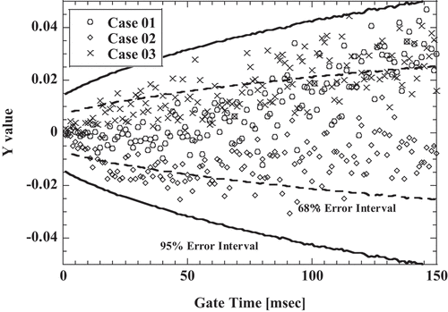
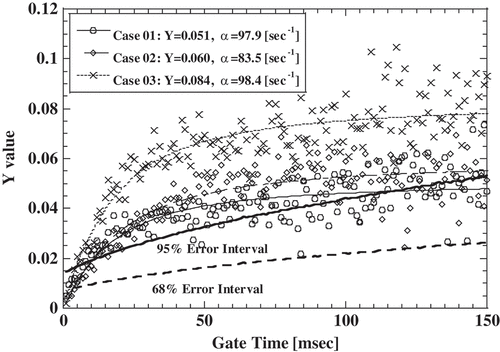
The calculation results of the Y value for Poisson event by the complete random method are shown in Figure 1, and the calculation results of the Y value for the bunching method are shown in Figure 2. A vertical axis is the Y value and a horizontal axis is the gate time width. Dashed lines are the error interval for 65% confidence interval, and the solid lines are the error interval for 95% confidence interval. The calculation was performed three times for each method. The Y value for the Poisson event is theoretically 0; however, the Y value by the bunching method can be seen to have a trend component that is not 0 dependent on the gate time width as shown in Figure 2. The trend component is different for each calculation, and the trend component is not seen in the processing result of the complete random method.

Figure 1. Complete random method’s process result for Y value.

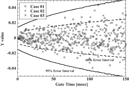
Figure 2. Bunching method’s process result for Y value.

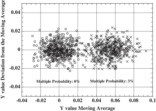
To investigate the characteristics of the trend component, the difference between the moving average of the gate time direction and the individual Y value and the moving average are plotted on a two-dimensional field. The number of samples of the moving average was 10 points, and the difference used the value in 100-msec gate time. Figure 3 shows a two-dimensional plot for the complete random method, and Figure 4 shows a two-dimensional plot for the bunching method. The vertical axis is the difference between the moving average value of Y value and Y value in the 100-msec gate time width, and the horizontal axis is the moving average of the Y value in the 100-msec gate time width. Plot points for the Poisson event are circle marks in Figures 3 and 4, and the number of plot point is 500 each. In the processing result of the bunching method, compared to that of the complete random method, the fluctuation of the difference is a little smaller, and it can be found that the fluctuation of the moving average is increased.

Figure 3. A two-dimensional plot of the moving average and the Y value – deviation for complete random method.

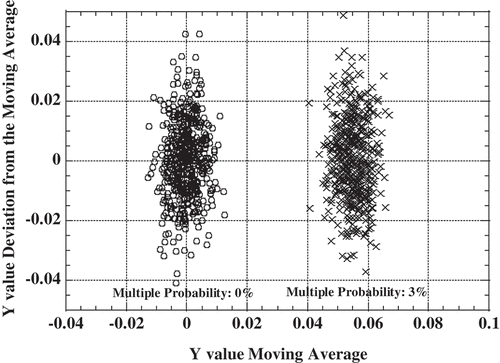
Figure 4. A two-dimensional plot of the moving average and the Y value – deviation for bunching method.

3.2 Analysis results for the multiplication events: 3％ multiplication probability

The calculation results of the Y value for the multiplication event by the complete random method are shown in Figure 5, and the calculation results of the Y value for the bunching method are shown in Figure 6. A vertical axis is the Y value and a horizontal axis is the gate time width. Dashed lines are the error interval for 65% confidence interval, and the solid lines are the error interval for 95% confidence interval. The calculation was performed three times for each method. The Y value is larger than the 95% error interval, but the processing result of the bunching method for 3% multiplication event has the same characteristics, the trend component, as for the Poisson event. For the results of the multiplication events, the difference between the moving average of the gate time direction and the individual Y value and the moving average are plotted on a two-dimensional field too. Two-dimensional plots for the multiplication events are cross marks in Figures 3 and 4, and the number of plot points is 500 each. It is easy to find from Figures 3 and 4 to have the same characteristics as the Poisson event in the case of 3% multiplication event.

Figure 5. Complete random method’s result of Y value for the multiplication events.

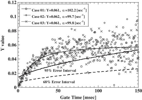
Figure 6. Bunching method’s result of Y value for the multiplication events.

4. Discussion and conclusion

Signal events based on the Poisson distribution and the multiplication phenomenon are simulated, and the processing results of the complete random method and the bunching method are compared in this paper. From the comparison, it became clear that the bunching method makes a trend component of Y value in the gate time width direction which the complete random method does not make.

The bunching method shared the same time series data for several gate time widths, and this is different from the Feynman’s recommended method. A method that some analysis time windows share the same time series data is very close to the wavelet technique [9]. Therefore, the trend component on the result of the bunching method is considered one of the periodicity information of the time series data.

Also, from the results of the two-dimensional plot, the bunching method was found to be a technique for increasing the fluctuation of the trend component instead of reducing the fluctuation of the Y value. This suggests that the bunching method could only replace the statistical fluctuation of the Y values with the fluctuation on the trend component.

When subjected to a very low-sensitive reactor noise measurement, not only negative trend components, there is also a possibility to have a positive trend component due to the periodicity information of the Poisson event. In this case, the positive trend component to be measured is a mixture of those caused by the fluctuation of the Poisson events and those due to the reactor information, and there is no method of separating the reactor component and the Poisson component of the Y value.

Ensuring that the Y value has a greater value than the error range to the variance-to-mean ratio of the Poisson statistics is a necessary process to determine that the Y value is not an accidental product. If the Y value is smaller than the error range for the variance-to-mean ratio of Poisson statistics, a re-experiment on conditions that yield a larger Y value or a re-experiment at a longer measurement time is necessary to get a larger Y value than the error range to the variance-to-mean ratio of the Poisson statistics.

Disclosure statement

No potential conflict of interest was reported by the authors.

Appendix

An error range of the variance-to-mean ratio for the Poisson events

This appendix gives a process to derive an error range of ‘the Variance-to-Mean Ratio’ for the Poisson events.

68% confidence interval, so-called a standard deviation, is generally used as an error interval for measured results of Poisson events. Here, 68% confidence interval of the variance-to-mean ratio is derived as an error interval for the Poisson events.

An error for a measured count, ΔN_i, is as follows:.

(A1) $\mathrm{\Delta }{N}_i=\sqrt{N_i}$(A1)

where N_i is a measured count of ith measurement. An average count, $\bar{N}$, is written as the following formulae:

(A2) $\bar{N}=\frac{{\sum }_{i=1}^n{N}_i}{n}$(A2)

where n is number of measurements.

Therefore, an error of the average count, Δ$\bar{N}$, is as follows:

(A3) $\begin{array}{ccc}\mathrm{\Delta }\bar{N}& =& \frac{\sqrt{{\left(\mathrm{\Delta }{N}_1\right)}^2+{\left(\mathrm{\Delta }{N}_2\right)}^2+\cdots +{\left(\mathrm{\Delta }{N}_n\right)}^2}}{n}\\ \hspace{0.17em}& =& \frac{\sqrt{{\sum }_{i=1}^n{N}_i}}{n}\\ \hspace{0.17em}& =& \sqrt{\frac{\bar{N}}{n}}\end{array}$(A3)

A deviation for an ith count, δ_i, is written as follows:

(A4) ${\delta }_i=N_i-\bar{N}$(A4)

Then, an error for the deviation, Δδ_i, becomes as follows:

(A5) $\begin{array}{ccc}\mathrm{\Delta }{\delta }_i& =& \sqrt{{\left(\mathrm{\Delta }{N}_i\right)}^2+{\left(\mathrm{\Delta }\bar{N}\right)}^2}\\ \hspace{0.17em}& =& \sqrt{{\left(\sqrt{N_i}\right)}^2+{\left(\sqrt{\frac{\bar{N}}{n}}\right)}^2}\\ \hspace{0.17em}& =& \sqrt{N_i+\frac{\bar{N}}{n}}\end{array}$(A5)

A variance, Var, is written with ${\delta }_i$ as follows:

(A6) $Var={\mu }_2=\sum _{i=1}^{i=n}{\delta }_i^2\cdot \frac{1}{n}$(A6)

An error of the square of the deviation, $\mathrm{\Delta }{\delta }_i^2$, is as follows:

(A7) $\begin{array}{ccc}\mathrm{\Delta }{\delta }_i^2& =& \sqrt{{\left\{\frac{d}{d{\delta }_i}\left({{\delta }_i}^2\right)\right\}}^2\cdot {\left(\mathrm{\Delta }{\delta }_i\right)}^2}\\ \hspace{0.17em}& =& 2\cdot {\delta }_i\cdot \mathrm{\Delta }{\delta }_i\\ \hspace{0.17em}& =& 2\cdot \left(N_i-\bar{N}\right)\cdot \sqrt{\frac{\bar{N}}{n}+N_i}\end{array}$(A7)

From this, an error of sum of the square deviation, $\mathrm{\Delta }\hspace{0.17em}\sum {\delta }^2$, is written as the following formulae:

(A8) $\begin{array}{rl}& \mathrm{\Delta }\sum {\delta }^2=\sqrt{{\left(\mathrm{\Delta }{\delta }_1\right)}^2+{\left(\mathrm{\Delta }{\delta }_2\right)}^2+\cdots +{\left(\mathrm{\Delta }{\delta }_n\right)}^2}\\ & =\sqrt{\frac{4}{n}}\cdot \sqrt{\sum _{i=1}^{i=n}\left(\bar{N}+n\cdot \le N_i\right)\cdot {\left(N_i-\bar{N}\right)}^2}\\ & =2\cdot \sqrt{n\cdot \overline{N^3}+\left(1-2\cdot n\right)\cdot \bar{N}\cdot \overline{N^2}+\left(n-1\right)\cdot {\left(\bar{N}\right)}^3}\end{array}$(A8)

Then, an error for the variance, $\mathrm{\Delta }Var$, is as follows:

(A9) $\begin{array}{l}\Delta Var=\Delta \frac{{\displaystyle \sum {\delta }^2}}{n}\\ =\frac{2}{n}\cdot \sqrt{n\cdot \overline{N^3+\left(1-2\cdot n\right)\cdot \overline{N}\cdot \overline{N^2}+\left(n-1\right)\cdot {\left(\overline{N}\right)}^3}}\end{array}$(A9)

An error for a variance-to-mean ratio, $\mathrm{\Delta }VtoM$, can be written as the following formulae:

(A10) $\mathrm{\Delta }VtoM=VtoM\cdot \sqrt{{\left(\frac{\mathrm{\Delta }Var}{Var}\right)}^2+{\left(\frac{\mathrm{\Delta }\bar{N}}{\bar{N}}\right)}^2}$(A10)

where $\mathrm{V}\mathrm{a}\mathrm{r}$ is a variance and $\mathrm{V}\mathrm{t}\mathrm{o}\mathrm{M}$ is a variance-to-mean ratio.

Here, when using the variance and average in the Poisson event is equal, (A10) can be deformed as follows:

(A11) $\begin{array}{rl}& \mathrm{\Delta }VtoM=\sqrt{{\left(\frac{\mathrm{\Delta }Var}{\bar{N}}\right)}^2+{\left(\frac{\mathrm{\Delta }\bar{N}}{\bar{N}}\right)}^2}\\ & =\frac{1}{\bar{N}}\cdot \sqrt{{\left(\mathrm{\Delta }Var\right)}^2+{\left(\mathrm{\Delta }\bar{N}\right)}^2}\\ & =\frac{1}{\bar{N}}\cdot \sqrt{\frac{4}{n^2}\cdot \left\{\begin{array}{c}n\cdot \overline{N^3}+\left(1-2\cdot n\right)\\ \cdot \bar{N}\cdot \overline{N^2}+\left(n-1\right)\cdot {\left(\bar{N}\right)}^3\end{array}\right\}+\frac{\bar{N}}{n}}\end{array}$(A11)

When using the bunching method, measured counts of ith sample-gate decrease with the shortening of the gate time width. Where the gate time width is shortened to the limit, N_i will take only 0 or 1. In this case, the mean value, square mean value, and cube mean value take the same value, and (A11) can be rewritten in the following formulae:

(A12) $\begin{array}{rl}& \mathrm{\Delta }VtoM=\frac{1}{\bar{N}}\cdot \sqrt{\frac{4}{n^2}\cdot \left\{\begin{array}{c}n\cdot \bar{N}+\left(1-2\cdot n\right)\cdot \bar{N}\cdot \bar{N}\\ +\left(n-1\right)\cdot {\left(\bar{N}\right)}^3\end{array}\right\}+\frac{\bar{N}}{n}}\\ & =\frac{1}{n\cdot \bar{N}}\cdot \sqrt{4\cdot \left\{\begin{array}{c}n\cdot \bar{N}+{\left(\bar{N}\right)}^2-2\cdot n\cdot \bar{N}\\ \cdot \bar{N}+n\cdot \bar{N}\cdot {\left(\bar{N}\right)}^2-{\left(\bar{N}\right)}^3\end{array}\right\}+n\cdot \bar{N}}\end{array}$(A12)

Here, the product of the number of gates and the average count is the same in the bunching method. (A12) becomes as follows:

(A13) $\begin{array}{l}\Delta VtoM=\frac{1}{C}\cdot \sqrt{4\cdot \left\{\begin{array}{l}C+{\left(\overline{N}\right)}^2-2\cdot C\cdot \overline{N}\\ +C\cdot {\left(\overline{N}\right)}^2-{\left(\overline{N}\right)}^3\end{array}\right\}+C}\\ =\frac{1}{C}\cdot \sqrt{5C-8C\cdot \overline{N}}+4\cdot \left(C+1\right)\cdot {\left(\overline{N}\right)}^2-4\cdot {\left(\overline{N}\right)}^3\end{array}$(A13)

$C=n\cdot \bar{N}$

Here, the gate time width is close to 0, that is, when the $\bar{N}$ is close to 0, (A13) becomes the following:

(A14) $\begin{array}{l}\underset{\overline{N}\to 0}{\lim }\Delta VtoM=\underset{\overline{N}\to 0}{\lim }\frac{1}{C}\cdot \sqrt{\begin{array}{l}5C-8C\cdot \overline{N}+4\cdot \left(C+1\right)\\ \cdot {\left(\overline{N}\right)}^2-4\cdot {\left(\overline{N}\right)}^3\end{array}}\\ =\sqrt{\frac{5}{C}}=\sqrt{\frac{5}{N_{total}}}\end{array}$(A14)

where $N_{total}$ is total counts of the measurements.

References

- Williams MMR. Random processes in nuclear reactors. Oxford (UK): Pergamon Press; 1974.
- Misawa T, Shiroya S, Kanda K. Measurement of prompt decay constant and subcriticality by the Feynman-α method. Nucl Sci Eng. 1990 Jan;104(1):53–65.
- Okuda R, Sakon A, Hohara S, et al. An improved Feynman-α analysis with a moving-bunching technique. J Nucl Sci Technol. 2016 Jan;53(10):1647–1652.
- Wada S, Yoshioka K, Kikuchi S Criticality control technique development for Fukushima Daiichi fuel debris, (31) debris uncertainty on sub-criticality estimation with Feynman-alpha method. Paper presented at: Atomic Energy Society of Japan 2017 Fall Meeting; 2017 Sep 13–15; Sapporo (Japan).
- Kano S, Oikawa M, Yazawa H Criticality control technique development for Fukushima Daiichi fuel debris, (32) operation verification of sub-criticality monitoring system using neutron source. Paper presented at: Atomic Energy Society of Japan 2017 Fall Meeting; 2017 Sep 13–15; Sapporo (Japan).
- Kano S, Wada S, Kikuchi S Criticality control technique development for Fukushima Daiichi fuel debris, (33) study on application of y∞ correlation equation of Feynman-alpha method to sub-criticality estimation of fuel debris. Paper presented at: Atomic Energy Society of Japan 2017 Fall Meeting; 2017 Sep 13–15; Sapporo (Japan).
- Knoll GF. Radiation detection and measurement. Fourth ed. New York (NY): John Wiley & Sons, Inc; 2010.
- Press WH, Teukolsky SA, Vetterling WT, et al. Numerical recipes in C. Second ed. Cambridge (UK): Cambridge University Press; 1992.
- Walker JS. A primer on WAVELETS and their scientific applications. Boca Raton (FL): Chapman & Hall/CRC; 1999.