Generalized formulation of extended cross-section adjustment method based on minimum variance unbiased linear estimation

ABSTRACT

By introducing a new assumption of linear estimation, we derive a new formulation of the extended cross-section adjustment (EA) method, which minimizes the variance of the design target core parameters. The new formulation is derived on the basis of minimum variance unbiased estimation with no use of the assumption of normal distribution. In this formulation, we found that EA has infinitely many solutions as the adjusted cross-section set. The new formulation of EA can represent all the possible solutions minimizing the variance of the design target core parameters and includes a special case identical to the classical Bayesian EA method, which was derived on the basis of the Bayes theorem under the assumption of normal distribution. Moreover, we prove that the special case minimizes not only the variance of the design target core parameters but also the variance of the nuclear data. Meanwhile, we show that the new assumption of linear estimation is consistent with the Kalman filter and demonstrate that we can formulate similarly the extended bias factor method, the conventional cross-section adjustment method, and the regressive cross-section adjustment method with no use of the assumption of normal distribution.

KEYWORDS:

• Kalman filter
• cross-section adjustment
• linear estimation
• minimum variance unbiased estimation
• Bayes theorem
• normal distribution
• uncertainty quantification
• nuclear data covariance

1. Introduction

As a neutronics design method for an innovative nuclear reactor system, the original cross-section adjustment methodology was established in 1970s–1980s [1–4]. With regard to the cross-section adjustment methodology, a comprehensive and detailed comparison study has been reported in references [5,6]. This methodology enables us to improve the prediction accuracy of neutronic characteristics by reducing uncertainties in nuclear data. In the cross-section adjustment methodology, the nuclear data are modified with the use of integral experimental quantities, such as measurement data acquired in critical experiments; the modified nuclear data are provided as an adjusted cross-section set for predicting the design target core parameters.

On the other hand, a formulation of the extended bias factor (EB) method [7] was proposed in 2007 as an alternative methodology for improving the prediction accuracy of the design target core parameters by using integral experimental quantities. In EB, a bias factor is obtained by a semifictitious experimental value, which is defined by a linear combination of integral experimental quantities; the design prediction value is corrected by the bias factor.

Subsequently, a formulation of the extended cross-section adjustment (EA) method [8] was proposed in 2012; EA can generate an adjusted cross-section set that reproduces the design prediction values and accuracies equivalent to EB. This formulation has revealed that EB minimizes the variance of the design prediction value of the target core parameter by considering cross-correlations in the analysis method error between the integral experimental quantities and the design target core parameters. Hence, in the case that there are strong cross-correlations in the analysis method error, EB can improve the design prediction accuracy more than the original cross-section adjustment methodology. Thus, the advantage of EB has been integrated into the cross-section adjustment methodology. In addition, the formulation of EA has revealed a difference between EA and EB. That is, the assumption of normal distribution required in the derivation of EA is not used in the derivation of EB. To explain this difference, the cross-section adjustment methods based on minimum variance unbiased estimation (MVUE) [9] were proposed in 2016. In reference [9], it has been shown that the MVUE-based rigorous extended cross-section adjustment (MREA) method, which was derived with no use of the assumption of normal distribution, can yield the design prediction values and accuracies equivalent to EB. Thus, it has been confirmed that the design prediction values and accuracies by EA are consistent with those by EB.

Moreover, the derivation of the MVUE-based cross-section adjustment methods [9] has clarified that the original cross-section adjustment methodology minimizes the variance of the nuclear data. This finding led to a formulation of the regressive cross-section adjustment (RA) method [9], which minimizes the variance of the integral experimental quantities. Although RA is unpractical as a neutronics design method, the formulation of RA is useful when we discuss what is optimized, that is, which variance is minimized, in the cross-section adjustment methodology. Thus, there are three variations of the cross-section adjustment methodology depending on the optimization target. In the present paper, we refer to the original cross-section adjustment methodology that minimizes the variance of the nuclear data as the conventional cross-section adjustment (CA) method. In particular, the original CA that was derived on the basis of the Bayes theorem under the assumption of normal distribution is called the classical Bayesian conventional cross-section adjustment (CBCA) method.

At that point in time, there was an unclear difference in the adjusted cross-section set with regard to CA. That is, the adjusted cross-section set by the MVUE-based rigorous conventional cross-section adjustment (MRCA) method [9], which was derived with no use of the assumption of normal distribution, differs from that by CBCA. In reference [9], it has been explained that a hypothetical mathematical operation, called ‘projection simplification,’ permits us to derive the MVUE-based simplified conventional cross-section adjustment (MSCA) method that can yield the adjusted cross-section set equivalent to CBCA. This explanation, however, is insufficient from the mathematical point of view. To explain this inconsistency in the adjusted cross-section sets between MRCA and CBCA, the dimension-reduced conventional cross-section adjustment (DRCA) method [10] was proposed in 2018. The derivation of DRCA has revealed that the formulation for the adjusted cross-section set equivalent to CBCA can be derived with no use of the assumption of normal distribution by introducing a concept of dimensionality reduction. Thus, the difference in the adjusted cross-section set has been explained mathematically with regard to CA.

As for EA, however, there remains a similar problem in the adjusted cross-section set. That is, the adjusted cross-section set by the MREA method [9], which was derived with no use of the assumption of normal distribution, differs from that by the classical Bayesian extended cross-section adjustment (CBEA) method [8], which was derived on the basis of the Bayes theorem under the assumption of normal distribution. Similarly to MSCA, the MVUE-based simplified extended cross-section adjustment (MSEA) method, which was derived by using the projection simplification, was proposed in reference [9] to explain the difference, but this explanation is also insufficient. Thus, it has not been clearly explained yet why this difference in the adjusted cross-section set is occurred with regard to EA.

In the present paper, with no use of the assumption of normal distribution, we derive a new formulation that can yield the adjusted cross-section set equivalent to CBEA. To derive the new formulation of EA, we focus attention on a fact that the formulation of the Kalman filter [11,12] can be derived with no use of the assumption of normal distribution. For this reason, we make a review on the derivation of the Kalman filter to clarify the relationship with the cross-section adjustment methodology. In accordance with this review, we introduce a new assumption of linear estimation into the derivation of the cross-section adjustment methods based on the MVUE. In the present paper, we refer to this derivation procedure based on MVUE with the use of the new assumption as minimum variance unbiased linear estimation (MVULE).

First, we derive the formulation of CA based on MVULE, namely, the MVULE-based conventional cross-section adjustment (MLCA) method. Next, we demonstrate that the formulation of EB can be also derived by the same procedure. That is, we formulate the MVULE-based extended bias factor (MLEB) method. Finally, we derive the formulation of the MVULE-based extended cross-section adjustment (MLEA) method and the MVULE-based regressive cross-section adjustment (MLRA) method.

In Section 2, we review the cross-section adjustment methods, the extended bias factor method, and the Kalman filter. In Section 3, the derivations of MLCA, MLEB, MLEA, and MLRA are described. In Section 4, we discuss the derived formulation and conclude in Section 5. The acronyms are described in the Abbreviations section at the end of this article.

2. Review

2.1. Review of cross-section adjustment method

2.1.1. Precondition

To review the formulation for the cross-section adjustment methodology, we first define the following numbers of data used in the methodology:

n_a: the number of nuclear data to be adjusted;

n⁽¹⁾: the number of integral experimental quantities used for adjustment; and

n⁽²⁾: the number of the design target core parameters to be considered in adjustment of EA.

In accordance with reference [9], MRCA is equivalent to CBCA under the condition of the overdetermined (well-posed) problem, where $n^{(1)}\ge n_a$ (cf. Section 4.1.2 in reference [9]). For this reason, we review the formulation under the condition of the underdetermined (ill-posed) problem, where $n^{(1)}<n_a$. With regard to EAs – including MREA, MSEA, and CBEA, a precondition that $n^{(2)}<n^{(1)}(<n_a)$ is adopted. As for DRCA, we focus on the special case equivalent to CBCA, namely, DRCA2 [10].

2.1.2. Unified formula

The adjusted cross-section set by the foregoing methods can be expressed in the unified form [9]:

(1) ${\mathbf{T}}_x\equiv {\mathbf{T}}_0+{\mathbf{B}}_x{\mathbf{D}}^{-1}\left({\mathbf{R}}_e^{(1)}-{\mathbf{R}}_c^{(1)}({\mathbf{T}}_0)\right),$(1)

where

(2) $B_x\equiv \{\begin{array}{l}M{G}^{(1)\text{T}}+G^{(2)+}{V}_m^{(12)\text{T}}\\ (x=\text{CBEA},\text{MSEA})\\ G^{(1)+}{\left(G^{(2)}{G}^{(1)+}\right)}^{+}\left(G^{(2)}M{G}^{(1)\text{T}}+V_m^{(12)\text{T}}\right)\\ (x=\text{MREA})\\ M{G}^{(1)\text{T}}\\ (x=\text{CBCA},\text{MSCA},\text{DRCA}2)\\ G^{(1)+}{G}^{(1)}M{G}^{(1)\text{T}}\\ (x=\text{MRCA}),\end{array}$(2)

(3) $\mathbf{D}\equiv {\mathbf{G}}^{(1)}\mathbf{M}{\mathbf{G}}^{(1)\mathrm{T}}+{\mathbf{V}}_{e+m}^{(1)},$(3)

and

(4) ${\mathbf{V}}_{e+m}^{(1)}\equiv {\mathbf{V}}_e^{(1)}+{\mathbf{V}}_m^{(1)}.$(4)

Here, we have defined as follows:

• ${\mathbf{T}}_0\in {\mathbb{R}}^{n_a\times 1}$: the unadjusted cross-section set;

• ${\mathbf{R}}_e^{(1)}\in {\mathbb{R}}^{n^{(1)}\times 1}$: the measurement value of the integral experimental quantities;

• ${\mathbf{R}}_c^{(1)}(\mathbf{T})\in {\mathbb{R}}^{n^{(1)}\times 1}$: the calculation value of the integral experimental quantities obtained using the cross-section set $\mathbf{T}$;

• ${\mathbf{G}}^{(1)}\in {\mathbb{R}}^{n^{(1)}\times n_a}$: the sensitivity coefficient matrix of the integral experimental quantities with respect to the nuclear data;

• ${\mathbf{G}}^{(2)}\in {\mathbb{R}}^{n^{(2)}\times n_a}$: the sensitivity coefficient matrix of the design target core parameters with respect to the nuclear data;

• $\mathbf{M}\in {\mathbb{R}}^{n_a\times n_a}$: the variance–covariance matrix of the unadjusted cross-section set;

• ${\mathbf{V}}_e^{(1)}\in {\mathbb{R}}^{n^{(1)}\times n^{(1)}}$: the variance–covariance matrix with respect to the experimental error;

• ${\mathbf{V}}_m^{(1)}\in {\mathbb{R}}^{n^{(1)}\times n^{(1)}}$: the variance–covariance matrix with respect to the analysis method error; and

• ${\mathbf{V}}_m^{(12)}\in {\mathbb{R}}^{n^{(1)}\times n^{(2)}}$: the cross-correlation matrix between the integral experimental quantities and the design target core parameters with respect to the analysis method error,

where $\mathfrak{X}\in {\mathbb{R}}^{m\times n}$ means that $\mathfrak{X}$ is an $m\times n$ real matrix. In addition, the superscript of ‘$+$’ denotes the Moore–Penrose pseudoinverse, and the superscript of ‘$\mathrm{T}$’ represents the matrix transpose. Note that $\mathbf{D}$ is the full variance–covariance matrix of the integral experimental quantities and is supposed to be invertible (i.e. nonsingular) since the inverse of $\mathbf{D}$ appears in Equation (1)(1) ${\mathbf{T}}_x\equiv {\mathbf{T}}_0+{\mathbf{B}}_x{\mathbf{D}}^{-1}\left({\mathbf{R}}_e^{(1)}-{\mathbf{R}}_c^{(1)}({\mathbf{T}}_0)\right),$(1) . Moreover, it is assumed that ${\mathbf{G}}^{(1)}$ and ${\mathbf{G}}^{(2)}$ have full rank. Then, recalling the precondition that $n^{(2)}<n^{(1)}<n_a$, we have

(5) ${\mathbf{G}}^{(i)}{\mathbf{G}}^{(i)+}=\mathbf{I}(i=1,2),$(5)

where $\mathbf{I}$ denotes the identity matrix.

In accordance with the formulation of the MVUE-based cross-section adjustment methods (cf. Equations (103)(103) $\begin{array}{rl}& {\mathbf{R}}_c^{(2)}(\hat{\mathbf{T}})={\mathbf{R}}_t^{(2)}+{\mathbf{G}}^{(2)}\mathbf{F}\left(\mathrm{\Delta }{\mathbf{e}}^{(1)}-\mathrm{\Delta }{\mathbf{m}}^{(1)}-{\mathbf{G}}^{(1)}\mathrm{\Delta }{\mathbf{T}}_0\right)\\ & +{\mathbf{G}}^{(2)}\mathrm{\Delta }{\mathbf{T}}_0+\mathrm{\Delta }{\mathbf{m}}^{(2)}\\ & ={\mathbf{R}}_t^{(2)}+\left({\mathbf{G}}^{(2)}-{\mathbf{G}}^{(2)}\mathbf{F}{\mathbf{G}}^{(1)}\right)\mathrm{\Delta }{\mathbf{T}}_0\\ & +{\mathbf{G}}^{(2)}\mathbf{F}\mathrm{\Delta }{\mathbf{e}}^{(1)}-{\mathbf{G}}^{(2)}\mathbf{F}\mathrm{\Delta }{\mathbf{m}}^{(1)}+\mathrm{\Delta }{\mathbf{m}}^{(2)}.\end{array}$(103) , (113)(113) ${\mathbf{G}}^{(2)\mathrm{T}}\left({\mathbf{G}}^{(2)}{\mathbf{F}}_{\mathrm{M}\mathrm{L}\mathrm{E}\mathrm{A}}-{\mathbf{G}}^{(2)}{\mathbf{B}}_{\mathrm{M}\mathrm{L}\mathrm{E}\mathrm{A}0}{\mathbf{D}}^{-1}\right)=\mathbf{O}.$(113) , and (112) in reference [9]), we can also write the variance-covariance matrix of the adjusted cross-section set, the variance of the calculation values of the integral experimental quantities reanalyzed using the adjusted cross-section set, and the variance of the prediction values of the design target core parameters in the unified forms:

(6) ${\mathbf{M}}_x=\mathbf{M}+{\mathbf{B}}_x{\mathbf{D}}^{-1}{\mathbf{B}}_x^{\mathrm{T}}-\mathbf{M}{\mathbf{G}}^{(1)\mathrm{T}}{\mathbf{D}}^{-1}{\mathbf{B}}_x^{\mathrm{T}}-{\mathbf{B}}_x{\mathbf{D}}^{-1}{\mathbf{G}}^{(1)}\mathbf{M},$(6)

(7) $\mathrm{V}\mathrm{a}\mathrm{r}\left({\mathbf{R}}_c^{(1)}({\mathbf{T}}_x)\right)={\mathbf{G}}^{(1)}{\mathbf{M}}_x{\mathbf{G}}^{(1)\mathrm{T}}+{\mathbf{V}}_m^{(1)}-{\mathbf{F}}_x{\mathbf{V}}_m^{(1)}-{\mathbf{V}}_m^{(1)}{\mathbf{F}}_x^{\mathrm{T}},$(7)

and

(8) $\mathrm{V}\mathrm{a}\mathrm{r}\left({\mathbf{R}}_c^{(2)}({\mathbf{T}}_x)\right)={\mathbf{G}}^{(2)}{\mathbf{M}}_x{\mathbf{G}}^{(2)\mathrm{T}}+{\mathbf{V}}_m^{(2)}-{\mathbf{L}}_x{\mathbf{V}}_m^{(12)}-{\mathbf{V}}_m^{(12)\mathrm{T}}{\mathbf{L}}_x^{\mathrm{T}},$(8)

respectively, where

(9) ${\mathbf{F}}_x\equiv {\mathbf{G}}^{(1)}{\mathbf{B}}_x{\mathbf{D}}^{-1},$(9)

and

(10) ${\mathbf{L}}_x\equiv {\mathbf{G}}^{(2)}{\mathbf{B}}_x{\mathbf{D}}^{-1}.$(10)

Here, we have defined as follows:

• $R_c^{(2)}(T)\in {ℝ}^{n^{(2)}\times 1}$: the calculation value of the design target core parameters obtained using the cross-section set $\mathbf{T}$; and

• $V_m^{(2)}\in {ℝ}^{n^{(2)}\times n^{(2)}}$: the variance–covariance matrix of the design target core parameters with respect to the analysis method error.

2.1.3. Detailed definition

In addition, let us define the following symbols:

• ${\mathbf{T}}_t\in {\mathbb{R}}^{n_a\times 1}$: the (unknown) true cross-section set;

• ${\mathbf{R}}_t^{(i)}\in {\mathbb{R}}^{n^{(i)}\times 1}$: the true value of integral experimental quantities ($i=1$) or of the design target core parameters ($i=2$);

• $\mathrm{\Delta }{\mathbf{T}}_0\in {\mathbb{R}}^{n_a\times 1}$: the error of the unadjusted cross-section set;

• $\mathrm{\Delta }{\mathbf{e}}^{(1)}\in {\mathbb{R}}^{n^{(1)}\times 1}$: the experimental error of the integral experimental quantities; and

• $\mathrm{\Delta }{\mathbf{m}}^{(i)}\in {\mathbb{R}}^{n^{(i)}\times 1}$: the analysis method error of the integral experimental quantities ($i=1$) or of the design target core parameters ($i=2$).

Then, some symbols can be redefined by

(11) ${\mathbf{G}}^{(i)}\equiv \frac{\mathrm{d}{\mathbf{R}}_c^{(i)}}{\mathrm{d}\mathbf{T}}{|}_{\mathbf{T}={\mathbf{T}}_0}(i=1,2),$(11)

(12) $\mathrm{\Delta }{\mathbf{T}}_0\equiv {\mathbf{T}}_0-{\mathbf{T}}_t,$(12)

(13) $\mathrm{\Delta }{\mathbf{e}}^{(1)}\equiv {\mathbf{R}}_e^{(1)}-{\mathbf{R}}_t^{(1)},$(13)

and

(14) $\mathrm{\Delta }{\mathbf{m}}^{(i)}\equiv {\mathbf{R}}_c^{(i)}({\mathbf{T}}_t)-{\mathbf{R}}_t^{(i)}(i=1,2).$(14)

Similarly, we can redefine the variance–covariance and cross-correlation matrices by

(15) $\mathbf{M}\equiv \mathrm{V}\mathrm{a}\mathrm{r}\left({\mathbf{T}}_0\right),$(15)

(16) ${\mathbf{V}}_e^{(1)}\equiv \mathrm{V}\mathrm{a}\mathrm{r}\left({\mathbf{R}}_e^{(1)}\right),$(16)

(17) ${\mathbf{V}}_m^{(i)}\equiv \mathrm{V}\mathrm{a}\mathrm{r}\left({\mathbf{R}}_c^{(i)}({\mathbf{T}}_t)\right)(i=1,2),$(17)

and

(18) ${\mathbf{V}}_m^{(ij)}\equiv \mathrm{C}\mathrm{o}\mathrm{v}\left({\mathbf{R}}_c^{(i)}({\mathbf{T}}_t),{\mathbf{R}}_c^{(j)}({\mathbf{T}}_t)\right)(i=1,2;j=1,2).$(18)

Here, we have defined $\mathrm{V}\mathrm{a}\mathrm{r}\left(\cdot \right)$ and $\mathrm{C}\mathrm{o}\mathrm{v}\left(\cdot \right)$ for column vectors $\mathfrak{X}$ and $\mathfrak{Y}$ by

(19) $\text{Var}\left(\mathfrak{X}\right)\equiv \text{E}\left(\left(\mathfrak{X}-\text{E}\left(\mathfrak{X}\right)\right){\left(\mathfrak{X}-\text{E}\left(\mathfrak{X}\right)\right)}^{\text{T}}\right),$(19)

and

(20) $\text{Cov}\left(\mathfrak{X},\mathfrak{Y}\right)\equiv \text{E}\left(\left(\mathfrak{X}-\text{E}\left(\mathfrak{X}\right)\right){\left(\mathfrak{Y}-\text{E}\left(\mathfrak{Y}\right)\right)}^{\text{T}}\right),$(20)

respectively, where $\mathrm{E}\left(\cdot \right)$ denotes the expectation value. Note that when $i=j$ in Equation (18)(18) ${\mathbf{V}}_m^{(ij)}\equiv \mathrm{C}\mathrm{o}\mathrm{v}\left({\mathbf{R}}_c^{(i)}({\mathbf{T}}_t),{\mathbf{R}}_c^{(j)}({\mathbf{T}}_t)\right)(i=1,2;j=1,2).$(18) , ${\mathbf{V}}_m^{(ii)}$ is reduced to ${\mathbf{V}}_m^{(i)}$ by definition. Moreover, all of the following variance-covariance matrices are symmetric:

(21) ${\mathbf{M}}^{\mathrm{T}}=\mathbf{M},$(21)

(22) ${\mathbf{V}}_e^{(1)\mathrm{T}}={\mathbf{V}}_e^{(1)},$(22)

and

(23) ${\mathbf{V}}_m^{(i)\mathrm{T}}={\mathbf{V}}_m^{(i)}.$(23)

On the other hand, a variance–covariance matrix is always nonnegative definite. That is, a variance-covariance matrix is either positive definite or positive semidefinite. Hence, $\mathbf{M}$, ${\mathbf{V}}_e^{(1)}$, and ${\mathbf{V}}_m^{(1)}$ are nonnegative definite. Moreover, ${\mathbf{G}}^{(1)}\mathbf{M}{\mathbf{G}}^{(1)\mathrm{T}}$, $\mathbf{D}$, and ${\mathbf{D}}^{-1}$ are symmetric and nonnegative definite in accordance with the following theorems:

• For an $n\times n$ matrix $\mathfrak{A}$ and an $n\times m$ matrix $\mathfrak{B}$, if $\mathfrak{A}$ is (symmetric and) nonnegative definite, ${\mathfrak{B}}^{\text{T}}\mathfrak{A}\mathfrak{B}$ is (symmetric and) nonnegative definite (e.g. Theorem 14.2.9 in reference [13]);

• For $n\times n$ matrices $\mathfrak{A}$ and $\mathfrak{B}$, if both $\mathfrak{A}$ and $\mathfrak{B}$ are nonnegative definite, $\mathfrak{A}+\mathfrak{B}$ is nonnegative definite (e.g. Lemma 14.2.4 in reference [13]); and

• For an $n\times n$ matrix $\mathfrak{A}$, if $\mathfrak{A}$ is invertible and symmetric, ${\mathfrak{A}}^{-1}$ is symmetric (e.g. Equation (2.4) in reference [13]);

• For an $n\times n$ matrix $\mathfrak{A}$, if $\mathfrak{A}$ is invertible and nonnegative definite, ${\mathfrak{A}}^{-1}$ is nonnegative definite (e.g. Corollary 14.2.11 in reference [13]).

2.2. Review of extended bias factor method

Given that the design prediction values by CBEA are equal to those by EB [8], the design prediction values by EB can be defined by

(24) ${\mathbf{R}}_{\mathrm{E}\mathrm{B}}^{(2)}\equiv {\mathbf{R}}_c^{(2)}({\mathbf{T}}_0)+\left({\mathbf{G}}^{(2)}\mathbf{M}{\mathbf{G}}^{(1)\mathrm{T}}+{\mathbf{V}}_m^{(12)\mathrm{T}}\right){\mathbf{D}}^{-1}\left({\mathbf{R}}_e^{(1)}-{\mathbf{R}}_c^{(1)}({\mathbf{T}}_0)\right).$(24)

This definition can be obtained by assuming linearity as it is done in Equation (75)(75) ${\mathbf{R}}_c^{(1)}({\mathbf{T}}^{\prime })-{\mathbf{R}}_c^{(1)}(\mathbf{T})\approx {\mathbf{G}}^{(1)}({\mathbf{T}}^{\prime }-\mathbf{T}).$(75) , which is described later, and substituting Equations (1)(1) ${\mathbf{T}}_x\equiv {\mathbf{T}}_0+{\mathbf{B}}_x{\mathbf{D}}^{-1}\left({\mathbf{R}}_e^{(1)}-{\mathbf{R}}_c^{(1)}({\mathbf{T}}_0)\right),$(1) and (2(2) $B_x\equiv \{\begin{array}{l}M{G}^{(1)\text{T}}+G^{(2)+}{V}_m^{(12)\text{T}}\\ (x=\text{CBEA},\text{MSEA})\\ G^{(1)+}{\left(G^{(2)}{G}^{(1)+}\right)}^{+}\left(G^{(2)}M{G}^{(1)\text{T}}+V_m^{(12)\text{T}}\right)\\ (x=\text{MREA})\\ M{G}^{(1)\text{T}}\\ (x=\text{CBCA},\text{MSCA},\text{DRCA}2)\\ G^{(1)+}{G}^{(1)}M{G}^{(1)\text{T}}\\ (x=\text{MRCA}),\end{array}$(2) ) as follows:

(25) $\begin{array}{rl}& {\mathbf{R}}_c^{(2)}({\mathbf{T}}_{\mathrm{C}\mathrm{B}\mathrm{E}\mathrm{A}})={\mathbf{R}}_c^{(2)}({\mathbf{T}}_0)+{\mathbf{G}}^{(2)}\left({\mathbf{T}}_{\mathrm{C}\mathrm{B}\mathrm{E}\mathrm{A}}-{\mathbf{T}}_0\right)\\ & ={\mathbf{R}}_c^{(2)}({\mathbf{T}}_0)+{\mathbf{G}}^{(2)}\\ & \left(\mathbf{M}{\mathbf{G}}^{(1)\mathrm{T}}+{\mathbf{G}}^{(2)+}{\mathbf{V}}_m^{(12)\mathrm{T}}\right){\mathbf{D}}^{-1}\\ & \left({\mathbf{R}}_e^{(1)}-{\mathbf{R}}_c^{(1)}({\mathbf{T}}_0)\right)={\mathbf{R}}_{\mathrm{E}\mathrm{B}}^{(2)},(25)\end{array}$(25)

where Equation (5)(5) ${\mathbf{G}}^{(i)}{\mathbf{G}}^{(i)+}=\mathbf{I}(i=1,2),$(5) is used.

2.3. Review of Kalman filter

Next, we review a derivation of the Kalman filter [14] and examine the relationship with the cross-section adjustment methodology.

2.3.1. Non-linear Kalman filter and its linearization

Let us consider the following equations as a nonlinear discrete-time state model for time series data:

(26) ${\mathbf{s}}_{k+1}=f({\mathbf{s}}_k)+{\mathbf{w}}_k,$(26)

(27) ${\mathbf{y}}_k=h({\mathbf{s}}_k)+{\mathbf{v}}_k,$(27)

where

• ${\mathbf{s}}_k\in {\mathbb{R}}^{n\times 1}$: the process state vector at time $t_k$;

• ${\mathbf{w}}_k\in {\mathbb{R}}^{n\times 1}$: the system error, which is a white noise contribution to the state vector for time interval $(t_{k+1},t_k)$;

• ${\mathit{y}}_k\in {\mathbb{R}}^{m\times 1}$: the measurement (observation vector) at time $t_k$;

• ${\mathit{v}}_k\in {\mathbb{R}}^{m\times 1}$: the measurement error at time $t_k$;

• $f(\cdot )$: the time-independent state transition function; and

• $h(\cdot )$: the time-independent observation function giving the ideal (noiseless) connection between the measurement and the state vector.

It is assumed that an approximate ${\mathbf{s}}_k^{\ast }$ can be determined by some means. When the difference between the actual and the approximate state vectors is defined by $\mathrm{\Delta }{\mathbf{s}}_k$, the actual state vector is written by

(28) ${\mathbf{s}}_k={\mathbf{s}}_k^{\ast }+\mathrm{\Delta }{\mathbf{s}}_k.$(28)

To linearize the equations of the discrete-time state model, let us approximate the state transition function and the observation function by the Taylor series expansion around ${\mathbf{s}}_k^{\ast }$:

(29) $f({\mathbf{s}}_k)\approx f({\mathbf{s}}_k^{\ast })+\frac{\mathrm{\partial }f}{\mathrm{\partial }{\mathbf{s}}_k}{|}_{{\mathbf{s}}_k={\mathbf{s}}_k^{\ast }}\mathrm{\Delta }{\mathbf{s}}_k,$(29)

and

(30) $h({\mathbf{s}}_k)\approx h({\mathbf{s}}_k^{\ast })+\frac{\mathrm{\partial }h}{\mathrm{\partial }{\mathbf{s}}_k}{|}_{{\mathbf{s}}_k={\mathbf{s}}_k^{\ast }}\mathrm{\Delta }{\mathbf{s}}_k,$(30)

where the higher-order terms are ignored. Thus, Equation (26)(26) ${\mathbf{s}}_{k+1}=f({\mathbf{s}}_k)+{\mathbf{w}}_k,$(26) can be written by

(31) ${\mathbf{s}}_{k+1}^{\ast }+\mathrm{\Delta }{\mathbf{s}}_{k+1}=f({\mathbf{s}}_k^{\ast })+{\mathrm{\Phi }}_k\mathrm{\Delta }{\mathbf{s}}_k+{\mathbf{w}}_k,$(31)

where

(32) ${\mathrm{\Phi }}_k\equiv \frac{\mathrm{\partial }f}{\mathrm{\partial }{\mathbf{s}}_k}{|}_{{\mathbf{s}}_k={\mathbf{s}}_k^{\ast }}\in {\mathbb{R}}^{n\times n}.$(32)

Meanwhile, when we need an approximation of the state vector at the next time step, we can adopt a transition of the approximate state vector at the previous time step. That is, ${\mathbf{s}}_{k+1}^{\ast }$ can be determined such that ${\mathbf{s}}_{k+1}^{\ast }=f({\mathbf{s}}_k^{\ast })$. Thus, Equation (31)(31) ${\mathbf{s}}_{k+1}^{\ast }+\mathrm{\Delta }{\mathbf{s}}_{k+1}=f({\mathbf{s}}_k^{\ast })+{\mathrm{\Phi }}_k\mathrm{\Delta }{\mathbf{s}}_k+{\mathbf{w}}_k,$(31) can be rewritten as

(33) $\mathrm{\Delta }{\mathbf{s}}_{k+1}={\mathrm{\Phi }}_k\mathrm{\Delta }{\mathbf{s}}_k+{\mathbf{w}}_k.$(33)

On the other hand, Equation (27)(27) ${\mathbf{y}}_k=h({\mathbf{s}}_k)+{\mathbf{v}}_k,$(27) can be expressed by

(34) ${\mathbf{y}}_k-h({\mathbf{s}}_k^{\ast })={\mathbf{H}}_k\mathrm{\Delta }{\mathbf{s}}_k+{\mathbf{v}}_k,$(34)

where

(35) ${\mathbf{H}}_k\equiv \frac{\mathrm{\partial }h}{\mathrm{\partial }{\mathbf{s}}_k}{|}_{{\mathbf{s}}_k={\mathbf{s}}_k^{\ast }}\in {\mathbb{R}}^{m\times n}.$(35)

To simplify the linearized model described by Equations (33)(33) $\mathrm{\Delta }{\mathbf{s}}_{k+1}={\mathrm{\Phi }}_k\mathrm{\Delta }{\mathbf{s}}_k+{\mathbf{w}}_k.$(33) and (34(34) ${\mathbf{y}}_k-h({\mathbf{s}}_k^{\ast })={\mathbf{H}}_k\mathrm{\Delta }{\mathbf{s}}_k+{\mathbf{v}}_k,$(34) ), we replace the state vector and the observation vector by

(36) ${\mathbf{x}}_k\equiv \mathrm{\Delta }{\mathbf{s}}_k={\mathbf{s}}_k-{\mathbf{s}}_k^{\ast },$(36)

and

(37) ${\mathbf{z}}_k\equiv {\mathbf{y}}_k-h({\mathbf{s}}_k^{\ast }),$(37)

respectively. Thus, the equations of the discrete-time state model can be rewritten as

(38) ${\mathbf{x}}_{k+1}={\mathrm{\Phi }}_k{\mathbf{x}}_k+{\mathbf{w}}_k,$(38)

(39) ${\mathbf{z}}_k={\mathbf{H}}_k{\mathbf{x}}_k+{\mathbf{v}}_k.$(39)

This formulation is known as the linear Kalman filter.

2.3.2. Linear Kalman filter

Next, we review the state model equations of the linear Kalman filter. The covariance matrices of the system noise and the observation noise are defined by

(40) $\mathrm{E}\left({\mathbf{w}}_k{\mathbf{w}}_i^{\mathrm{T}}\right)=\left\{\begin{array}{c}{\mathbf{Q}}_k(i=k)\\ \mathbf{O}(i\ne k),\end{array}\right.$(40)

(41) $\mathrm{E}\left({\mathbf{v}}_k{\mathbf{v}}_i^{\mathrm{T}}\right)=\left\{\begin{array}{c}{\mathbf{R}}_k(i=k)\\ \mathbf{O}(i\ne k),\end{array}\right.$(41)

and

(42) $\mathrm{E}\left({\mathbf{w}}_k{\mathbf{v}}_i^{\mathrm{T}}\right)=\mathbf{O}\hspace{0.17em}(\mathrm{f}\mathrm{o}\mathrm{r}\mathrm{a}\mathrm{l}\mathrm{l}k\mathrm{a}\mathrm{n}\mathrm{d}i),$(42)

where $\mathbf{O}$ denotes the zero matrix. Let us denote the prior estimate by ${\hat{\mathbf{x}}}_{k0}$, which is the state vector estimated from the information prior to time $t_k$, where the hat $({}^{\wedge })$ represents an estimate, and the subscript of ‘$0$’ means an estimate prior to assimilating the measurement at time $t_k$.

Let us assume that the covariance matrix of the prior estimate is known. That is, the estimation error is defined explicitly by

(43) ${\mathbf{e}}_{k0}\equiv {\mathbf{x}}_k-{\hat{\mathbf{x}}}_{k0},$(43)

then the covariance matrix of the prior estimate can be written by

(44) ${\mathbf{P}}_{k0}=\mathrm{E}\left({\mathbf{e}}_{k0}{\mathbf{e}}_{k0}^{\mathrm{T}}\right)=\mathrm{E}\left(\left({\mathbf{x}}_k-{\hat{\mathbf{x}}}_{k0}\right){\left({\mathbf{x}}_k-{\hat{\mathbf{x}}}_{k0}\right)}^{\mathrm{T}}\right).$(44)

Next, let us consider improving the prior estimate by using the measurement at time $t_k$. For this purpose, a linear blending of the measurement ${\mathbf{z}}_k$ and the prior estimate ${\hat{\mathbf{x}}}_{k0}$ is adopted in the form:

(45) ${\hat{\mathbf{x}}}_k={\hat{\mathbf{x}}}_{k0}+{\mathbf{K}}_k\left({\mathbf{z}}_k-{\mathbf{H}}_k{\hat{\mathbf{x}}}_{k0}\right),$(45)

where

${\hat{\mathbf{x}}}_k$: the updated estimate of the state vector and

${\mathbf{K}}_k$: the linear blending factor.

Meanwhile, the covariance matrix of the updated estimate is expressed by

(46) ${\mathbf{P}}_k=\mathrm{E}\left({\mathbf{e}}_k{\mathbf{e}}_k^{\mathrm{T}}\right)=\mathrm{E}\left(\left({\mathbf{x}}_k-{\hat{\mathbf{x}}}_k\right){\left({\mathbf{x}}_k-{\hat{\mathbf{x}}}_k\right)}^{\mathrm{T}}\right).$(46)

Substituting Equation (39)(39) ${\mathbf{z}}_k={\mathbf{H}}_k{\mathbf{x}}_k+{\mathbf{v}}_k.$(39) into Equation (45)(45) ${\hat{\mathbf{x}}}_k={\hat{\mathbf{x}}}_{k0}+{\mathbf{K}}_k\left({\mathbf{z}}_k-{\mathbf{H}}_k{\hat{\mathbf{x}}}_{k0}\right),$(45) yields

(47) ${\hat{\mathbf{x}}}_k={\hat{\mathbf{x}}}_{k0}+{\mathbf{K}}_k\left({\mathbf{H}}_k{\mathbf{x}}_k+{\mathbf{v}}_k-{\mathbf{H}}_k{\hat{\mathbf{x}}}_{k0}\right).$(47)

Thus, substituting Equation (47)(47) ${\hat{\mathbf{x}}}_k={\hat{\mathbf{x}}}_{k0}+{\mathbf{K}}_k\left({\mathbf{H}}_k{\mathbf{x}}_k+{\mathbf{v}}_k-{\mathbf{H}}_k{\hat{\mathbf{x}}}_{k0}\right).$(47) in Equation (46)(46) ${\mathbf{P}}_k=\mathrm{E}\left({\mathbf{e}}_k{\mathbf{e}}_k^{\mathrm{T}}\right)=\mathrm{E}\left(\left({\mathbf{x}}_k-{\hat{\mathbf{x}}}_k\right){\left({\mathbf{x}}_k-{\hat{\mathbf{x}}}_k\right)}^{\mathrm{T}}\right).$(46) and considering that there is no correlation between ${\mathbf{e}}_{k0}$ and ${\mathbf{v}}_k$, we obtain

(48) $\begin{array}{rl}& {\mathbf{P}}_k=\mathrm{E}\left(\left(\left({\mathbf{x}}_k-{\hat{\mathbf{x}}}_{k0}\right)-{\mathbf{K}}_k\left({\mathbf{H}}_k{\mathbf{x}}_k+{\mathbf{v}}_k-{\mathbf{H}}_k{\hat{\mathbf{x}}}_{k0}\right)\right)\right.\\ & \left.{\left(\left({\mathbf{x}}_k-{\hat{\mathbf{x}}}_{k0}\right)-{\mathbf{K}}_k\left({\mathbf{H}}_k{\mathbf{x}}_k+{\mathbf{v}}_k-{\mathbf{H}}_k{\hat{\mathbf{x}}}_{k0}\right)\right)}^{\mathrm{T}}\right)\\ & =\mathrm{E}\left(\left({\mathbf{e}}_{k0}-{\mathbf{K}}_k\left({\mathbf{H}}_k{\mathbf{e}}_{k0}+{\mathbf{v}}_k\right)\right){\left({\mathbf{e}}_{k0}-{\mathbf{K}}_k\left({\mathbf{H}}_k{\mathbf{e}}_{k0}+{\mathbf{v}}_k\right)\right)}^{\mathrm{T}}\right)\\ & =\left(\mathbf{I}-{\mathbf{K}}_k{\mathbf{H}}_k\right)\mathrm{E}\left({\mathbf{e}}_{k0}{\mathbf{e}}_{k0}^{\mathrm{T}}\right){\left(\mathbf{I}-{\mathbf{K}}_k{\mathbf{H}}_k\right)}^{\mathrm{T}}+{\mathbf{K}}_k\mathrm{E}\left({\mathbf{v}}_k{\mathbf{v}}_k^{\mathrm{T}}\right){\mathbf{K}}_k^{\mathrm{T}}\\ & =\left(\mathbf{I}-{\mathbf{K}}_k{\mathbf{H}}_k\right){\mathbf{P}}_{k0}{\left(\mathbf{I}-{\mathbf{K}}_k{\mathbf{H}}_k\right)}^{\mathrm{T}}+{\mathbf{K}}_k{\mathbf{R}}_k{\mathbf{K}}_k^{\mathrm{T}}\\ & ={\mathbf{P}}_{k0}-{\mathbf{K}}_k{\mathbf{H}}_k{\mathbf{P}}_{k0}-{\mathbf{P}}_{k0}{\mathbf{H}}_k^{\mathrm{T}}{\mathbf{K}}_k^{\mathrm{T}}+{\mathbf{K}}_k\left({\mathbf{H}}_k{\mathbf{P}}_{k0}{\mathbf{H}}_k^{\mathrm{T}}+{\mathbf{R}}_k\right){\mathbf{K}}_k^{\mathrm{T}}.\end{array}$(48)

To derive this equation, we have used that the following equation holds for arbitrary matrices $\mathfrak{A}$ and $\mathfrak{B}$:

(49) ${\left(\mathfrak{A}\mathfrak{B}\right)}^{\text{T}}={\mathfrak{B}}^{\text{T}}{\mathfrak{A}}^{\text{T}}.$(49)

To determine the blending factor that minimizes the trace of the covariance matrix of the updated estimate, we consider the partial derivative:

(50) $\begin{array}{rl}& \frac{\mathrm{\partial }}{\mathrm{\partial }{\mathbf{K}}_k}\mathrm{t}\mathrm{r}\left({\mathbf{P}}_k\right)=-2\frac{\mathrm{\partial }}{\mathrm{\partial }{\mathbf{K}}_k}\mathrm{t}\mathrm{r}\left({\mathbf{P}}_{k0}{\mathbf{H}}_k^{\mathrm{T}}{\mathbf{K}}_k^{\mathrm{T}}\right)\\ & +\frac{\mathrm{\partial }}{\mathrm{\partial }{\mathbf{K}}_k}\mathrm{t}\mathrm{r}\left({\mathbf{K}}_k\left({\mathbf{H}}_k{\mathbf{P}}_{k0}{\mathbf{H}}_k^{\mathrm{T}}+{\mathbf{R}}_k\right){\mathbf{K}}_k^{\mathrm{T}}\right)\\ & =-2{\mathbf{P}}_{k0}{\mathbf{H}}_k^{\mathrm{T}}+2{\mathbf{K}}_k\left({\mathbf{H}}_k{\mathbf{P}}_{k0}{\mathbf{H}}_k^{\mathrm{T}}+{\mathbf{R}}_k\right),\end{array}$(50)

where $\mathrm{t}\mathrm{r}\left(\cdot \right)$ denotes the matrix trace, which is the sum of the diagonal elements. To derive Equation (50)(50) $\begin{array}{rl}& \frac{\mathrm{\partial }}{\mathrm{\partial }{\mathbf{K}}_k}\mathrm{t}\mathrm{r}\left({\mathbf{P}}_k\right)=-2\frac{\mathrm{\partial }}{\mathrm{\partial }{\mathbf{K}}_k}\mathrm{t}\mathrm{r}\left({\mathbf{P}}_{k0}{\mathbf{H}}_k^{\mathrm{T}}{\mathbf{K}}_k^{\mathrm{T}}\right)\\ & +\frac{\mathrm{\partial }}{\mathrm{\partial }{\mathbf{K}}_k}\mathrm{t}\mathrm{r}\left({\mathbf{K}}_k\left({\mathbf{H}}_k{\mathbf{P}}_{k0}{\mathbf{H}}_k^{\mathrm{T}}+{\mathbf{R}}_k\right){\mathbf{K}}_k^{\mathrm{T}}\right)\\ & =-2{\mathbf{P}}_{k0}{\mathbf{H}}_k^{\mathrm{T}}+2{\mathbf{K}}_k\left({\mathbf{H}}_k{\mathbf{P}}_{k0}{\mathbf{H}}_k^{\mathrm{T}}+{\mathbf{R}}_k\right),\end{array}$(50) , we have used the following equations for arbitrary matrices $\mathfrak{A}$ and $\mathfrak{B}$:

(51) $\text{tr}\left(\mathfrak{A}+\mathfrak{B}\right)=\text{tr}\left(\mathfrak{A}\right)+\text{tr}\left(\mathfrak{B}\right),$(51)

and

(52) $\text{tr}\left({\mathfrak{A}}^{\text{T}}\right)=\text{tr}\left(\mathfrak{A}\right).$(52)

Moreover, we have used the following derivative formulas for arbitrary constant matrices $\mathfrak{A}$, $\mathfrak{B}$, $\mathfrak{C}$:

(53) $\frac{\mathrm{\partial }}{\mathrm{\partial }\mathfrak{X}}\left(\mathrm{t}\mathrm{r}\left(\mathfrak{A}\right)+\mathrm{t}\mathrm{r}\left(\mathfrak{B}\right)\right)=\frac{\mathrm{\partial }}{\mathrm{\partial }\mathfrak{X}}\mathrm{t}\mathrm{r}\left(\mathfrak{A}\right)+\frac{\mathrm{\partial }}{\mathrm{\partial }\mathfrak{X}}\mathrm{t}\mathrm{r}\left(\mathfrak{B}\right),$(53)

(54) $\frac{\mathrm{\partial }}{\mathrm{\partial }\mathfrak{X}}\mathrm{t}\mathrm{r}\left(\mathfrak{A}{\mathfrak{X}}^{\mathrm{T}}\mathfrak{B}\right)=\mathfrak{B}\mathfrak{A},$(54)

and

(55) $\frac{\mathrm{\partial }}{\mathrm{\partial }\mathfrak{X}}\mathrm{t}\mathrm{r}\left(\mathfrak{A}\mathfrak{X}\mathfrak{B}{\mathfrak{X}}^{\mathrm{T}}\mathfrak{C}\right)={\mathfrak{A}}^{\mathrm{T}}{\mathfrak{C}}^{\mathrm{T}}\mathfrak{X}{\mathfrak{B}}^{\mathrm{T}}+\mathfrak{C}\mathfrak{A}\mathfrak{X}\mathfrak{B}.$(55)

To determine the blending factor that minimizes the trace of ${\mathbf{P}}_k$, we set Equation (50)(50) $\begin{array}{rl}& \frac{\mathrm{\partial }}{\mathrm{\partial }{\mathbf{K}}_k}\mathrm{t}\mathrm{r}\left({\mathbf{P}}_k\right)=-2\frac{\mathrm{\partial }}{\mathrm{\partial }{\mathbf{K}}_k}\mathrm{t}\mathrm{r}\left({\mathbf{P}}_{k0}{\mathbf{H}}_k^{\mathrm{T}}{\mathbf{K}}_k^{\mathrm{T}}\right)\\ & +\frac{\mathrm{\partial }}{\mathrm{\partial }{\mathbf{K}}_k}\mathrm{t}\mathrm{r}\left({\mathbf{K}}_k\left({\mathbf{H}}_k{\mathbf{P}}_{k0}{\mathbf{H}}_k^{\mathrm{T}}+{\mathbf{R}}_k\right){\mathbf{K}}_k^{\mathrm{T}}\right)\\ & =-2{\mathbf{P}}_{k0}{\mathbf{H}}_k^{\mathrm{T}}+2{\mathbf{K}}_k\left({\mathbf{H}}_k{\mathbf{P}}_{k0}{\mathbf{H}}_k^{\mathrm{T}}+{\mathbf{R}}_k\right),\end{array}$(50) equal to zero and solve for ${\mathbf{K}}_k$. The result is

(56) ${\mathbf{K}}_k={\mathbf{P}}_{k0}{\mathbf{H}}_k^{\mathrm{T}}{\left({\mathbf{H}}_k{\mathbf{P}}_{k0}{\mathbf{H}}_k^{\mathrm{T}}+{\mathbf{R}}_k\right)}^{-1}.$(56)

This equation is called the Kalman gain. Substituting this equation into Equation (45)(45) ${\hat{\mathbf{x}}}_k={\hat{\mathbf{x}}}_{k0}+{\mathbf{K}}_k\left({\mathbf{z}}_k-{\mathbf{H}}_k{\hat{\mathbf{x}}}_{k0}\right),$(45) , we obtain

(57) ${\hat{\mathbf{x}}}_k={\hat{\mathbf{x}}}_{k0}+{\mathbf{P}}_{k0}{\mathbf{H}}_k^{\mathrm{T}}{\left({\mathbf{H}}_k{\mathbf{P}}_{k0}{\mathbf{H}}_k^{\mathrm{T}}+{\mathbf{R}}_k\right)}^{-1}\left({\mathbf{z}}_k-{\mathbf{H}}_k{\hat{\mathbf{x}}}_{k0}\right).$(57)

This equation enables us to estimate the state vector at time $t_k$.

2.3.3. Relationship with cross-section adjustment method

As defined by Equations (1)(1) ${\mathbf{T}}_x\equiv {\mathbf{T}}_0+{\mathbf{B}}_x{\mathbf{D}}^{-1}\left({\mathbf{R}}_e^{(1)}-{\mathbf{R}}_c^{(1)}({\mathbf{T}}_0)\right),$(1) – (3(3) $\mathbf{D}\equiv {\mathbf{G}}^{(1)}\mathbf{M}{\mathbf{G}}^{(1)\mathrm{T}}+{\mathbf{V}}_{e+m}^{(1)},$(3) ), the adjusted cross-section set by CBCA is written by

(58) $\begin{array}{rl}& {\mathbf{T}}_{\mathrm{C}\mathrm{B}\mathrm{C}\mathrm{A}}={\mathbf{T}}_0+\mathbf{M}{\mathbf{G}}^{(1)\mathrm{T}}\\ & {\left({\mathbf{G}}^{(1)}\mathbf{M}{\mathbf{G}}^{(1)\mathrm{T}}+{\mathbf{V}}_{e+m}^{(1)}\right)}^{-1}\left({\mathbf{R}}_e^{(1)}-{\mathbf{R}}_c^{(1)}({\mathbf{T}}_0)\right).\end{array}$(58)

Although this equation is similar to Equation (57)(57) ${\hat{\mathbf{x}}}_k={\hat{\mathbf{x}}}_{k0}+{\mathbf{P}}_{k0}{\mathbf{H}}_k^{\mathrm{T}}{\left({\mathbf{H}}_k{\mathbf{P}}_{k0}{\mathbf{H}}_k^{\mathrm{T}}+{\mathbf{R}}_k\right)}^{-1}\left({\mathbf{z}}_k-{\mathbf{H}}_k{\hat{\mathbf{x}}}_{k0}\right).$(57) , it differs from Equation (57)(57) ${\hat{\mathbf{x}}}_k={\hat{\mathbf{x}}}_{k0}+{\mathbf{P}}_{k0}{\mathbf{H}}_k^{\mathrm{T}}{\left({\mathbf{H}}_k{\mathbf{P}}_{k0}{\mathbf{H}}_k^{\mathrm{T}}+{\mathbf{R}}_k\right)}^{-1}\left({\mathbf{z}}_k-{\mathbf{H}}_k{\hat{\mathbf{x}}}_{k0}\right).$(57) in that it deals with the nonlinearity of ${\mathbf{R}}_c^{(1)}(\cdot )$. To eliminate this difference, let us consider the following correspondence in light of the derivation procedure for linearizing the Kalman filter:

(59) ${\hat{\mathbf{x}}}_k={\hat{\mathbf{s}}}_k-{\mathbf{s}}_k^{\ast }\leftrightarrow {\mathbf{T}}_{\mathrm{C}\mathrm{B}\mathrm{C}\mathrm{A}}-{\mathbf{T}}_0,$(59)

(60) ${\hat{\mathbf{x}}}_{k0}={\hat{\mathbf{s}}}_{k0}-{\mathbf{s}}_k^{\ast }\leftrightarrow {\mathbf{T}}_0-{\mathbf{T}}_0(=\mathbf{O}),$(60)

(61) ${\mathbf{z}}_k={\mathbf{y}}_k-h({\mathbf{s}}_k^{\ast })\leftrightarrow {\mathbf{R}}_e^{(1)}-{\mathbf{R}}_c^{(1)}({\mathbf{T}}_0),$(61)

(62) ${\mathbf{P}}_{k0}\leftrightarrow \mathbf{M},$(62)

(63) ${\mathbf{H}}_k\leftrightarrow {\mathbf{G}}^{(1)},$(63)

and

(64) ${\mathbf{R}}_k\leftrightarrow {\mathbf{V}}_{e+m}^{(1)}.$(64)

Thus, we can understand that Equation (58)(58) $\begin{array}{rl}& {\mathbf{T}}_{\mathrm{C}\mathrm{B}\mathrm{C}\mathrm{A}}={\mathbf{T}}_0+\mathbf{M}{\mathbf{G}}^{(1)\mathrm{T}}\\ & {\left({\mathbf{G}}^{(1)}\mathbf{M}{\mathbf{G}}^{(1)\mathrm{T}}+{\mathbf{V}}_{e+m}^{(1)}\right)}^{-1}\left({\mathbf{R}}_e^{(1)}-{\mathbf{R}}_c^{(1)}({\mathbf{T}}_0)\right).\end{array}$(58) is identical to Equation (57)(57) ${\hat{\mathbf{x}}}_k={\hat{\mathbf{x}}}_{k0}+{\mathbf{P}}_{k0}{\mathbf{H}}_k^{\mathrm{T}}{\left({\mathbf{H}}_k{\mathbf{P}}_{k0}{\mathbf{H}}_k^{\mathrm{T}}+{\mathbf{R}}_k\right)}^{-1}\left({\mathbf{z}}_k-{\mathbf{H}}_k{\hat{\mathbf{x}}}_{k0}\right).$(57) .

Moreover, in light of Equation (64)(64) ${\mathbf{R}}_k\leftrightarrow {\mathbf{V}}_{e+m}^{(1)}.$(64) , we can find another correspondence:

(65) ${\mathbf{v}}_k\leftrightarrow -\mathrm{\Delta }{\mathbf{e}}^{(1)}+\mathrm{\Delta }{\mathbf{m}}^{(1)}.$(65)

From this correspondence, we can understand that the cross-section adjustment method is a linearized model of the nonlinear Kalman filter described by the state model equations:

(66) ${\mathbf{T}}_1=f({\mathbf{T}}_0)+{\mathbf{w}}_0,$(66)

(67) ${\mathbf{R}}_e^{(1)}+\mathrm{\Delta }{\mathbf{e}}^{(1)}={\mathbf{R}}_c^{(1)}({\mathbf{T}}_0)+\mathrm{\Delta }{\mathbf{m}}^{(1)},$(67)

where ${\mathbf{T}}_1$ represents the cross-section set at time $t_1$. Although Equation (66)(66) ${\mathbf{T}}_1=f({\mathbf{T}}_0)+{\mathbf{w}}_0,$(66) is inessential for the cross-section adjustment methodology, the state model described by Equation (67)(67) ${\mathbf{R}}_e^{(1)}+\mathrm{\Delta }{\mathbf{e}}^{(1)}={\mathbf{R}}_c^{(1)}({\mathbf{T}}_0)+\mathrm{\Delta }{\mathbf{m}}^{(1)},$(67) is reasonable as the observation of C/E (calculation/experiment) values for the integral experimental quantities. On the other hand, since the linearization of the nonlinear Kalman filter is known as the extended Kalman filter (EKF), we can understand that the cross-section adjustment methodology is a kind of EKF.

2.4. Discussion on assumption of linear estimation

As described before, the Kalman gain is determined by minimizing the variance with no use of the assumption of normal distribution. This procedure is similar to determining the linear combination factor $\mathbf{F}$ in the derivation of the MVUE-based cross-section adjustment methods. Hence, we can find yet another correspondence:

(68) ${\mathbf{K}}_k\leftrightarrow \mathbf{F}.$(68)

Substituting the foregoing correspondence, that is, Equations (59)(59) ${\hat{\mathbf{x}}}_k={\hat{\mathbf{s}}}_k-{\mathbf{s}}_k^{\ast }\leftrightarrow {\mathbf{T}}_{\mathrm{C}\mathrm{B}\mathrm{C}\mathrm{A}}-{\mathbf{T}}_0,$(59) – (61(61) ${\mathbf{z}}_k={\mathbf{y}}_k-h({\mathbf{s}}_k^{\ast })\leftrightarrow {\mathbf{R}}_e^{(1)}-{\mathbf{R}}_c^{(1)}({\mathbf{T}}_0),$(61) ), and (68(68) ${\mathbf{K}}_k\leftrightarrow \mathbf{F}.$(68) ), into Equation (45)(45) ${\hat{\mathbf{x}}}_k={\hat{\mathbf{x}}}_{k0}+{\mathbf{K}}_k\left({\mathbf{z}}_k-{\mathbf{H}}_k{\hat{\mathbf{x}}}_{k0}\right),$(45) , we obtain

(69) $\hat{\mathbf{T}}-{\mathbf{T}}_0=\mathbf{F}\left({\mathbf{R}}_e^{(1)}-{\mathbf{R}}_c^{(1)}({\mathbf{T}}_0)\right).$(69)

This equation differs from the following equation that represents the assumption of linear estimation used in the derivation of the MVUE-based cross-section adjustment methods [9]:

(70) ${\hat{\mathbf{R}}}^{(1)}-{\mathbf{R}}_c^{(1)}({\mathbf{T}}_0)=\mathbf{F}\left({\mathbf{R}}_e^{(1)}-{\mathbf{R}}_c^{(1)}({\mathbf{T}}_0)\right).$(70)

In light of the review of the Kalman filter, it is expected that we can formulate a new cross-section adjustment method if we adopt Equation (69)(69) $\hat{\mathbf{T}}-{\mathbf{T}}_0=\mathbf{F}\left({\mathbf{R}}_e^{(1)}-{\mathbf{R}}_c^{(1)}({\mathbf{T}}_0)\right).$(69) as the assumption of linear estimation.

On the other hand, we can use another equation as the assumption of linear estimation. That is, if we consider the design target core parameters as the state vector, the assumption of linear estimation can be written by

(71) ${\hat{\mathbf{R}}}^{(2)}-{\mathbf{R}}_c^{(2)}({\mathbf{T}}_0)=\mathbf{F}\left({\mathbf{R}}_e^{(1)}-{\mathbf{R}}_c^{(1)}({\mathbf{T}}_0)\right).$(71)

Since this equation estimates directly the design target core parameters, it is expected that a new formulation corresponding to EB can be derived if Equation (71)(71) ${\hat{\mathbf{R}}}^{(2)}-{\mathbf{R}}_c^{(2)}({\mathbf{T}}_0)=\mathbf{F}\left({\mathbf{R}}_e^{(1)}-{\mathbf{R}}_c^{(1)}({\mathbf{T}}_0)\right).$(71) is used as the assumption of linear estimation.

In the following, we derive MLCA with the use of Equation (69)(69) $\hat{\mathbf{T}}-{\mathbf{T}}_0=\mathbf{F}\left({\mathbf{R}}_e^{(1)}-{\mathbf{R}}_c^{(1)}({\mathbf{T}}_0)\right).$(69) as the assumption of linear estimation. Subsequently, MLEB is derived by using Equation (71)(71) ${\hat{\mathbf{R}}}^{(2)}-{\mathbf{R}}_c^{(2)}({\mathbf{T}}_0)=\mathbf{F}\left({\mathbf{R}}_e^{(1)}-{\mathbf{R}}_c^{(1)}({\mathbf{T}}_0)\right).$(71) . Finally, we derive MLEA and MLRA with Equation (69)(69) $\hat{\mathbf{T}}-{\mathbf{T}}_0=\mathbf{F}\left({\mathbf{R}}_e^{(1)}-{\mathbf{R}}_c^{(1)}({\mathbf{T}}_0)\right).$(69) .

3. Derivation

3.1. Assumptions

In the present paper, we adopt the same assumptions used in the derivation of the MVUE-based cross-section adjustment methods [9] except for the assumption of linear estimation. However, since these assumptions are essential for the formulation, we summarize them in the following.

3.1.1. Assumptions on number of data

Unlike the foregoing review of the cross-section adjustment methods, we employ no particular assumption (precondition) regarding the relationship between the number of integral experimental quantities and the number of nuclear data:

(72) $n^{(1)}\frac{>}{<}{n}_{\mathrm{a}}.$(72)

That is, it is unnecessary to distinguish whether the problem is overdetermined or underdetermined in the present formulation. With regard to EA, it is assumed that the number of design target core parameters is smaller than the number of nuclear data:

(73) $n^{(2)}<n_a.$(73)

In addition, we assume that ${\mathbf{G}}^{(2)}$ has full rank:

(74) $\mathrm{r}\mathrm{a}\mathrm{n}\mathrm{k}\left({\mathbf{G}}^{(2)}\right)=n^{(2)}.$(74)

Note that ${\mathbf{G}}^{(2)}$ is a wide matrix and has full row rank in light of Equations (73)(73) $n^{(2)}<n_a.$(73) and (74(74) $\mathrm{r}\mathrm{a}\mathrm{n}\mathrm{k}\left({\mathbf{G}}^{(2)}\right)=n^{(2)}.$(74) ). By contrast, at this moment, we pay no attention to whether ${\mathbf{G}}^{(1)}$ is of full rank.

3.1.2. Assumption of linearity

Let us assume that the variation of two calculation values obtained by different cross-section sets ${\mathbf{T}}^{\prime }$ and $\mathbf{T}$ can be evaluated by the first-order approximation in the form:

(75) ${\mathbf{R}}_c^{(1)}({\mathbf{T}}^{\prime })-{\mathbf{R}}_c^{(1)}(\mathbf{T})\approx {\mathbf{G}}^{(1)}({\mathbf{T}}^{\prime }-\mathbf{T}).$(75)

Then, the difference between the experimental value and the calculation value of integral experimental quantities can be expressed by

(76) $\begin{array}{rl}& {\mathbf{R}}_e^{(1)}-{\mathbf{R}}_c^{(1)}({\mathbf{T}}_0)=\left({\mathbf{R}}_e^{(1)}-{\mathbf{R}}_t^{(1)}\right)-\left({\mathbf{R}}_c^{(1)}({\mathbf{T}}_t)-{\mathbf{R}}_t^{(1)}\right)\\ & -\left({\mathbf{R}}_c^{(1)}({\mathbf{T}}_0)-{\mathbf{R}}_c^{(1)}({\mathbf{T}}_t)\right)\approx \mathrm{\Delta }{\mathbf{e}}^{(1)}\\ & -\mathrm{\Delta }{\mathbf{m}}^{(1)}-{\mathbf{G}}^{(1)}\mathrm{\Delta }{\mathbf{T}}_0,\end{array}$(76)

where Equations(13) $\mathrm{\Delta }{\mathbf{e}}^{(1)}\equiv {\mathbf{R}}_e^{(1)}-{\mathbf{R}}_t^{(1)},$(13) (12(12) $\mathrm{\Delta }{\mathbf{T}}_0\equiv {\mathbf{T}}_0-{\mathbf{T}}_t,$(12) )–(14(14) $\mathrm{\Delta }{\mathbf{m}}^{(i)}\equiv {\mathbf{R}}_c^{(i)}({\mathbf{T}}_t)-{\mathbf{R}}_t^{(i)}(i=1,2).$(14) ) are used.

3.1.3. Assumption of unbiased estimation

Let us assume that the unbiased estimation is valid all for the nuclear data included in the unadjusted cross-section set, the experimental value and the calculation value of the integral experimental quantities, and the calculation value of the design target core parameters. That is, we assume that the expectation value is equal to the true value:

(77) $\mathrm{E}\left({\mathbf{T}}_0\right)={\mathbf{T}}_t,$(77)

(78) $\mathrm{E}\left({\mathbf{R}}_e^{(1)}\right)={\mathbf{R}}_t^{(1)},$(78)

and

(79) $\mathrm{E}\left({\mathbf{R}}_c^{(i)}({\mathbf{T}}_t)\right)={\mathbf{R}}_t^{(i)}(i=1,2).$(79)

Then, in light of Equations (19)(19) $\text{Var}\left(\mathfrak{X}\right)\equiv \text{E}\left(\left(\mathfrak{X}-\text{E}\left(\mathfrak{X}\right)\right){\left(\mathfrak{X}-\text{E}\left(\mathfrak{X}\right)\right)}^{\text{T}}\right),$(19) and (20(20) $\text{Cov}\left(\mathfrak{X},\mathfrak{Y}\right)\equiv \text{E}\left(\left(\mathfrak{X}-\text{E}\left(\mathfrak{X}\right)\right){\left(\mathfrak{Y}-\text{E}\left(\mathfrak{Y}\right)\right)}^{\text{T}}\right),$(20) ), the foregoing covariance and cross-correlation matrices can be rewritten as

(80) $\mathbf{M}=\mathrm{E}\left(\mathrm{\Delta }{\mathbf{T}}_0\mathrm{\Delta }{\mathbf{T}}_0^{\mathrm{T}}\right),$(80)

(81) ${\mathbf{V}}_e^{(1)}=\mathrm{E}\left(\mathrm{\Delta }{\mathbf{e}}^{(1)}\mathrm{\Delta }{\mathbf{e}}^{(1)\mathrm{T}}\right),$(81)

(82) ${\mathbf{V}}_m^{(i)}=\mathrm{E}\left(\mathrm{\Delta }{\mathbf{m}}^{(i)}\mathrm{\Delta }{\mathbf{m}}^{(i)\mathrm{T}}\right)(i=1,2),$(82)

and

(83) ${\mathbf{V}}_m^{(ij)}=\mathrm{E}\left(\mathrm{\Delta }{\mathbf{m}}^{(i)}\mathrm{\Delta }{\mathbf{m}}^{(j)\mathrm{T}}\right)(i=1,2;j=1,2).$(83)

3.1.4. Assumption of error independence

Moreover, we assume that the experimental error, the analysis method error, and the cross-section-induced errors with respect to the integral experimental quantities and the design target core parameters are independent of each other:

(84) $\mathrm{E}\left(\mathrm{\Delta }{\mathbf{x}}_i\mathrm{\Delta }{\mathbf{x}}_j^{\mathrm{T}}\right)=\mathbf{O}(i\ne j),$(84)

where

(85) $\mathrm{\Delta }{\mathbf{x}}_i\equiv \left\{\begin{array}{c}\mathrm{\Delta }{\mathbf{e}}^{(1)}(i=1)\\ \mathrm{\Delta }{\mathbf{m}}^{(1)},\mathrm{\Delta }{\mathbf{m}}^{(2)}(i=2)\\ {\mathbf{G}}^{(1)}\mathrm{\Delta }{\mathbf{T}}_0(i=3)\\ {\mathbf{G}}^{(2)}\mathrm{\Delta }{\mathbf{T}}_0(i=4).\end{array}\right.$(85)

3.2. Derivation of conventional cross-section adjustment method

Let us derive MLCA by using Equation (69)(69) $\hat{\mathbf{T}}-{\mathbf{T}}_0=\mathbf{F}\left({\mathbf{R}}_e^{(1)}-{\mathbf{R}}_c^{(1)}({\mathbf{T}}_0)\right).$(69) as the assumption of linear estimation.

3.2.1. Derivation of adjusted cross-section set

In light of Equation (12)(12) $\mathrm{\Delta }{\mathbf{T}}_0\equiv {\mathbf{T}}_0-{\mathbf{T}}_t,$(12) , the estimate of the cross-section set can be written by

(86) $\hat{\mathbf{T}}={\mathbf{T}}_t+(\hat{\mathbf{T}}-{\mathbf{T}}_0)+\mathrm{\Delta }{\mathbf{T}}_0.$(86)

Substituting Equations (69)(69) $\hat{\mathbf{T}}-{\mathbf{T}}_0=\mathbf{F}\left({\mathbf{R}}_e^{(1)}-{\mathbf{R}}_c^{(1)}({\mathbf{T}}_0)\right).$(69) and (76(76) $\begin{array}{rl}& {\mathbf{R}}_e^{(1)}-{\mathbf{R}}_c^{(1)}({\mathbf{T}}_0)=\left({\mathbf{R}}_e^{(1)}-{\mathbf{R}}_t^{(1)}\right)-\left({\mathbf{R}}_c^{(1)}({\mathbf{T}}_t)-{\mathbf{R}}_t^{(1)}\right)\\ & -\left({\mathbf{R}}_c^{(1)}({\mathbf{T}}_0)-{\mathbf{R}}_c^{(1)}({\mathbf{T}}_t)\right)\approx \mathrm{\Delta }{\mathbf{e}}^{(1)}\\ & -\mathrm{\Delta }{\mathbf{m}}^{(1)}-{\mathbf{G}}^{(1)}\mathrm{\Delta }{\mathbf{T}}_0,\end{array}$(76) ) in Equation (86)(86) $\hat{\mathbf{T}}={\mathbf{T}}_t+(\hat{\mathbf{T}}-{\mathbf{T}}_0)+\mathrm{\Delta }{\mathbf{T}}_0.$(86) , we have

(87) $\begin{array}{c}\hat{\mathbf{T}}={\mathbf{T}}_t+\mathbf{F}\left(\mathrm{\Delta }{\mathbf{e}}^{(1)}-\mathrm{\Delta }{\mathbf{m}}^{(1)}-{\mathbf{G}}^{(1)}\mathrm{\Delta }{\mathbf{T}}_0\right)+\mathrm{\Delta }{\mathbf{T}}_0\\ ={\mathbf{T}}_t+\left(\mathbf{I}-\mathbf{F}{\mathbf{G}}^{(1)}\right)\mathrm{\Delta }{\mathbf{T}}_0+\mathbf{F}\mathrm{\Delta }{\mathbf{e}}^{(1)}-\mathbf{F}\mathrm{\Delta }{\mathbf{m}}^{(1)}.\end{array}$(87)

Thus, the variance of $\hat{\mathbf{T}}$ can be expressed by

(88) $\begin{array}{rl}& \mathrm{V}\mathrm{a}\mathrm{r}\left(\hat{\mathbf{T}}\right)=\mathrm{E}\left(\left(\hat{\mathbf{T}}-{\mathbf{T}}_t\right){\left(\hat{\mathbf{T}}-{\mathbf{T}}_t\right)}^{\mathrm{T}}\right)\\ & =\left(\mathbf{I}-\mathbf{F}{\mathbf{G}}^{(1)}\right)\mathrm{E}\left(\mathrm{\Delta }{\mathbf{T}}_0\mathrm{\Delta }{\mathbf{T}}_0^{\mathrm{T}}\right){\left(\mathbf{I}-\mathbf{F}{\mathbf{G}}^{(1)}\right)}^{\mathrm{T}}\\ & +\mathbf{F}\mathrm{E}\left(\mathrm{\Delta }{\mathbf{e}}^{(1)}\mathrm{\Delta }{\mathbf{e}}^{(1)\mathrm{T}}\right)\mathbf{F}+\mathbf{F}\mathrm{E}\left(\mathrm{\Delta }{\mathbf{m}}^{(1)}\mathrm{\Delta }{\mathbf{m}}^{(1)\mathrm{T}}\right)\mathbf{F}\\ & =\mathbf{M}+\mathbf{F}{\mathbf{G}}^{(1)}\mathbf{M}{\mathbf{G}}^{(1)\mathrm{T}}{\mathbf{F}}^{\mathrm{T}}-\mathbf{M}{\mathbf{G}}^{(1)\mathrm{T}}{\mathbf{F}}^{\mathrm{T}}\\ & -\mathbf{F}{\mathbf{G}}^{(1)}\mathbf{M}+{\mathbf{F}\mathbf{V}}_e^{(1)}{\mathbf{F}}^{\mathrm{T}}+{\mathbf{F}\mathbf{V}}_m^{(1)}{\mathbf{F}}^{\mathrm{T}}\\ & =\mathbf{M}+\mathbf{F}\left({\mathbf{G}}^{(1)}\mathbf{M}{\mathbf{G}}^{(1)\mathrm{T}}+{\mathbf{V}}_{e+m}^{(1)}\right){\mathbf{F}}^{\mathrm{T}}\\ & -\mathbf{M}{\mathbf{G}}^{(1)\mathrm{T}}{\mathbf{F}}^{\mathrm{T}}-{\left(\mathbf{M}{\mathbf{G}}^{(1)\mathrm{T}}{\mathbf{F}}^{\mathrm{T}}\right)}^{\mathrm{T}}\end{array}$(88)

where Equations(84) $\mathrm{E}\left(\mathrm{\Delta }{\mathbf{x}}_i\mathrm{\Delta }{\mathbf{x}}_j^{\mathrm{T}}\right)=\mathbf{O}(i\ne j),$(84) (84(84) $\mathrm{E}\left(\mathrm{\Delta }{\mathbf{x}}_i\mathrm{\Delta }{\mathbf{x}}_j^{\mathrm{T}}\right)=\mathbf{O}(i\ne j),$(84) ), (80(80) $\mathbf{M}=\mathrm{E}\left(\mathrm{\Delta }{\mathbf{T}}_0\mathrm{\Delta }{\mathbf{T}}_0^{\mathrm{T}}\right),$(80) ), (81(81) ${\mathbf{V}}_e^{(1)}=\mathrm{E}\left(\mathrm{\Delta }{\mathbf{e}}^{(1)}\mathrm{\Delta }{\mathbf{e}}^{(1)\mathrm{T}}\right),$(81) ), (82(82) ${\mathbf{V}}_m^{(i)}=\mathrm{E}\left(\mathrm{\Delta }{\mathbf{m}}^{(i)}\mathrm{\Delta }{\mathbf{m}}^{(i)\mathrm{T}}\right)(i=1,2),$(82) ) and (4(4) ${\mathbf{V}}_{e+m}^{(1)}\equiv {\mathbf{V}}_e^{(1)}+{\mathbf{V}}_m^{(1)}.$(4) ) are used. To determine the linear combination factor $\mathbf{F}$ that minimizes the variance, let us consider the partial derivative of the trace of this variance with respect to $\mathbf{F}$:

(89) $\begin{array}{rl}& \frac{\mathrm{\partial }}{\mathrm{\partial }\mathbf{F}}\mathrm{t}\mathrm{r}\left(\mathrm{V}\mathrm{a}\mathrm{r}\left(\hat{\mathbf{T}}\right)\right)=\frac{\mathrm{\partial }}{\mathrm{\partial }\mathbf{F}}\mathrm{t}\mathrm{r}\left(\mathbf{F}\left({\mathbf{G}}^{(1)}\mathbf{M}{\mathbf{G}}^{(1)\mathrm{T}}+{\mathbf{V}}_{e+m}^{(1)}\right){\mathbf{F}}^{\mathrm{T}}\right)\\ & -2\frac{\mathrm{\partial }}{\mathrm{\partial }\mathbf{F}}\mathrm{t}\mathrm{r}\left(\mathbf{M}{\mathbf{G}}^{(1)\mathrm{T}}{\mathbf{F}}^{\mathrm{T}}\right)\\ & =2\mathbf{F}\left({\mathbf{G}}^{(1)}\mathbf{M}{\mathbf{G}}^{(1)\mathrm{T}}+{\mathbf{V}}_{e+m}^{(1)}\right)-2\mathbf{M}{\mathbf{G}}^{(1)\mathrm{T}}\end{array}$(89)

where Equations (51)(51) $\text{tr}\left(\mathfrak{A}+\mathfrak{B}\right)=\text{tr}\left(\mathfrak{A}\right)+\text{tr}\left(\mathfrak{B}\right),$(51) –(55(55) $\frac{\mathrm{\partial }}{\mathrm{\partial }\mathfrak{X}}\mathrm{t}\mathrm{r}\left(\mathfrak{A}\mathfrak{X}\mathfrak{B}{\mathfrak{X}}^{\mathrm{T}}\mathfrak{C}\right)={\mathfrak{A}}^{\mathrm{T}}{\mathfrak{C}}^{\mathrm{T}}\mathfrak{X}{\mathfrak{B}}^{\mathrm{T}}+\mathfrak{C}\mathfrak{A}\mathfrak{X}\mathfrak{B}.$(55) ) are used. It is possible to determine the linear combination factor matrix $\mathbf{F}$ that minimizes the variance by setting Equation (89)(89) $\begin{array}{rl}& \frac{\mathrm{\partial }}{\mathrm{\partial }\mathbf{F}}\mathrm{t}\mathrm{r}\left(\mathrm{V}\mathrm{a}\mathrm{r}\left(\hat{\mathbf{T}}\right)\right)=\frac{\mathrm{\partial }}{\mathrm{\partial }\mathbf{F}}\mathrm{t}\mathrm{r}\left(\mathbf{F}\left({\mathbf{G}}^{(1)}\mathbf{M}{\mathbf{G}}^{(1)\mathrm{T}}+{\mathbf{V}}_{e+m}^{(1)}\right){\mathbf{F}}^{\mathrm{T}}\right)\\ & -2\frac{\mathrm{\partial }}{\mathrm{\partial }\mathbf{F}}\mathrm{t}\mathrm{r}\left(\mathbf{M}{\mathbf{G}}^{(1)\mathrm{T}}{\mathbf{F}}^{\mathrm{T}}\right)\\ & =2\mathbf{F}\left({\mathbf{G}}^{(1)}\mathbf{M}{\mathbf{G}}^{(1)\mathrm{T}}+{\mathbf{V}}_{e+m}^{(1)}\right)-2\mathbf{M}{\mathbf{G}}^{(1)\mathrm{T}}\end{array}$(89) equal to zero. Let ${\mathbf{F}}_{\mathrm{M}\mathrm{L}\mathrm{C}\mathrm{A}}$ denote the minimizing factor of $\mathbf{F}$, then we have

(90) ${\mathbf{F}}_{\mathrm{M}\mathrm{L}\mathrm{C}\mathrm{A}}\left({\mathbf{G}}^{(1)}\mathbf{M}{\mathbf{G}}^{(1)\mathrm{T}}+{\mathbf{V}}_{e+m}^{(1)}\right)=\mathbf{M}{\mathbf{G}}^{(1)\mathrm{T}}.$(90)

Premultiplying both sides of this equation by the inverse of $\mathbf{D}$ defined by Equation (3)(3) $\mathbf{D}\equiv {\mathbf{G}}^{(1)}\mathbf{M}{\mathbf{G}}^{(1)\mathrm{T}}+{\mathbf{V}}_{e+m}^{(1)},$(3) , we obtain

(91) ${\mathbf{F}}_{\mathrm{M}\mathrm{L}\mathrm{C}\mathrm{A}}=\mathbf{M}{\mathbf{G}}^{(1)\mathrm{T}}{\mathbf{D}}^{-1}$(91)

Substituting ${\mathbf{F}}_{\mathrm{M}\mathrm{L}\mathrm{C}\mathrm{A}}$ into $\mathbf{F}$ in Equation (69)(69) $\hat{\mathbf{T}}-{\mathbf{T}}_0=\mathbf{F}\left({\mathbf{R}}_e^{(1)}-{\mathbf{R}}_c^{(1)}({\mathbf{T}}_0)\right).$(69) and defining ${\mathbf{T}}_{\mathrm{M}\mathrm{L}\mathrm{C}\mathrm{A}}$ in this case as $\hat{\mathbf{T}}$, we have

(92) ${\mathbf{T}}_{\mathrm{M}\mathrm{L}\mathrm{C}\mathrm{A}}={\mathbf{T}}_0+\mathbf{M}{\mathbf{G}}^{(1)\mathrm{T}}{\mathbf{D}}^{-1}\left({\mathbf{R}}_e^{(1)}-{\mathbf{R}}_c^{(1)}({\mathbf{T}}_0)\right).$(92)

This equation is identical to that for the adjusted cross-section set by CBCA:

(93) ${\mathbf{T}}_{\mathrm{M}\mathrm{L}\mathrm{C}\mathrm{A}}={\mathbf{T}}_{\mathrm{C}\mathrm{B}\mathrm{C}\mathrm{A}}.$(93)

In summary, if Equation (69)(69) $\hat{\mathbf{T}}-{\mathbf{T}}_0=\mathbf{F}\left({\mathbf{R}}_e^{(1)}-{\mathbf{R}}_c^{(1)}({\mathbf{T}}_0)\right).$(69) is valid as the assumption of linear estimation, we can derive the formula identical to CBCA by using neither the projection simplification nor the concept of dimensionality reduction.

3.2.2. Derivation of variances

Given that Equations (6)(6) ${\mathbf{M}}_x=\mathbf{M}+{\mathbf{B}}_x{\mathbf{D}}^{-1}{\mathbf{B}}_x^{\mathrm{T}}-\mathbf{M}{\mathbf{G}}^{(1)\mathrm{T}}{\mathbf{D}}^{-1}{\mathbf{B}}_x^{\mathrm{T}}-{\mathbf{B}}_x{\mathbf{D}}^{-1}{\mathbf{G}}^{(1)}\mathbf{M},$(6) –(8(8) $\mathrm{V}\mathrm{a}\mathrm{r}\left({\mathbf{R}}_c^{(2)}({\mathbf{T}}_x)\right)={\mathbf{G}}^{(2)}{\mathbf{M}}_x{\mathbf{G}}^{(2)\mathrm{T}}+{\mathbf{V}}_m^{(2)}-{\mathbf{L}}_x{\mathbf{V}}_m^{(12)}-{\mathbf{V}}_m^{(12)\mathrm{T}}{\mathbf{L}}_x^{\mathrm{T}},$(8) ) can be derived with no use of the assumption of linear estimation (cf. Sections 4.2–4.4 in reference [9]), we can adopt these equations also in MLCA. Thus, we can understand that the prediction accuracies by MLCA are also equivalent to CBCA.

3.3. Derivation of extended bias factor method

Next, let us derive MLEB by using Equation (71)(71) ${\hat{\mathbf{R}}}^{(2)}-{\mathbf{R}}_c^{(2)}({\mathbf{T}}_0)=\mathbf{F}\left({\mathbf{R}}_e^{(1)}-{\mathbf{R}}_c^{(1)}({\mathbf{T}}_0)\right).$(71) as the assumption of linear estimation.

3.3.1. Derivation of estimate of design target core parameters

The calculation values of the design target core parameters obtained using the unadjusted cross-section set can be written by

(94) $\begin{array}{rl}& {\mathbf{R}}_c^{(2)}({\mathbf{T}}_0)={\mathbf{R}}_t^{(2)}+\left({\mathbf{R}}_c^{(2)}({\mathbf{T}}_0)-{\mathbf{R}}_c^{(2)}({\mathbf{T}}_t)\right)\\ & +\left({\mathbf{R}}_c^{(2)}({\mathbf{T}}_t)-{\mathbf{R}}_t^{(2)}\right)\approx {\mathbf{R}}_t^{(2)}+{\mathbf{G}}^{(2)}({\mathbf{T}}_0-{\mathbf{T}}_t)\\ & +\mathrm{\Delta }{\mathbf{m}}^{(2)}={\mathbf{R}}_t^{(2)}+{\mathbf{G}}^{(2)}\mathrm{\Delta }{\mathbf{T}}_0+\mathrm{\Delta }{\mathbf{m}}^{(2)},\end{array}$(94)

where Equations (75)(75) ${\mathbf{R}}_c^{(1)}({\mathbf{T}}^{\prime })-{\mathbf{R}}_c^{(1)}(\mathbf{T})\approx {\mathbf{G}}^{(1)}({\mathbf{T}}^{\prime }-\mathbf{T}).$(75) , (14(14) $\mathrm{\Delta }{\mathbf{m}}^{(i)}\equiv {\mathbf{R}}_c^{(i)}({\mathbf{T}}_t)-{\mathbf{R}}_t^{(i)}(i=1,2).$(14) ), and (12(12) $\mathrm{\Delta }{\mathbf{T}}_0\equiv {\mathbf{T}}_0-{\mathbf{T}}_t,$(12) ) are used. Substituting Equations (94)(94) $\begin{array}{rl}& {\mathbf{R}}_c^{(2)}({\mathbf{T}}_0)={\mathbf{R}}_t^{(2)}+\left({\mathbf{R}}_c^{(2)}({\mathbf{T}}_0)-{\mathbf{R}}_c^{(2)}({\mathbf{T}}_t)\right)\\ & +\left({\mathbf{R}}_c^{(2)}({\mathbf{T}}_t)-{\mathbf{R}}_t^{(2)}\right)\approx {\mathbf{R}}_t^{(2)}+{\mathbf{G}}^{(2)}({\mathbf{T}}_0-{\mathbf{T}}_t)\\ & +\mathrm{\Delta }{\mathbf{m}}^{(2)}={\mathbf{R}}_t^{(2)}+{\mathbf{G}}^{(2)}\mathrm{\Delta }{\mathbf{T}}_0+\mathrm{\Delta }{\mathbf{m}}^{(2)},\end{array}$(94) and (76(76) $\begin{array}{rl}& {\mathbf{R}}_e^{(1)}-{\mathbf{R}}_c^{(1)}({\mathbf{T}}_0)=\left({\mathbf{R}}_e^{(1)}-{\mathbf{R}}_t^{(1)}\right)-\left({\mathbf{R}}_c^{(1)}({\mathbf{T}}_t)-{\mathbf{R}}_t^{(1)}\right)\\ & -\left({\mathbf{R}}_c^{(1)}({\mathbf{T}}_0)-{\mathbf{R}}_c^{(1)}({\mathbf{T}}_t)\right)\approx \mathrm{\Delta }{\mathbf{e}}^{(1)}\\ & -\mathrm{\Delta }{\mathbf{m}}^{(1)}-{\mathbf{G}}^{(1)}\mathrm{\Delta }{\mathbf{T}}_0,\end{array}$(76) ) in Equation (71)(71) ${\hat{\mathbf{R}}}^{(2)}-{\mathbf{R}}_c^{(2)}({\mathbf{T}}_0)=\mathbf{F}\left({\mathbf{R}}_e^{(1)}-{\mathbf{R}}_c^{(1)}({\mathbf{T}}_0)\right).$(71) , we have

(95) $\begin{array}{rl}& {\hat{\mathbf{R}}}^{(2)}={\mathbf{R}}_t^{(2)}+{\mathbf{G}}^{(2)}\mathrm{\Delta }{\mathbf{T}}_0+\mathrm{\Delta }{\mathbf{m}}^{(2)}\\ & +\mathbf{F}\left(\mathrm{\Delta }{\mathbf{e}}^{(1)}-\mathrm{\Delta }{\mathbf{m}}^{(1)}-{\mathbf{G}}^{(1)}\mathrm{\Delta }{\mathbf{T}}_0\right)\\ & ={\mathbf{R}}_t^{(2)}+\left({\mathbf{G}}^{(2)}-\mathbf{F}{\mathbf{G}}^{(1)}\right)\mathrm{\Delta }{\mathbf{T}}_0+\mathbf{F}\mathrm{\Delta }{\mathbf{e}}^{(1)}\\ & -\mathbf{F}\mathrm{\Delta }{\mathbf{m}}^{(1)}+\mathrm{\Delta }{\mathbf{m}}^{(2)}.(95)\end{array}$(95)

Thus, the variance of ${\hat{\mathbf{R}}}^{(2)}$ can be written by

(96) $\begin{array}{rl}& \mathrm{V}\mathrm{a}\mathrm{r}\left({\hat{\mathbf{R}}}^{(2)}\right)=\mathrm{E}\left(\left({\hat{\mathbf{R}}}^{(2)}-{\mathbf{R}}_t^{(2)}\right){\left({\hat{\mathbf{R}}}^{(2)}-{\mathbf{R}}_t^{(2)}\right)}^{\mathrm{T}}\right)\\ & =\left({\mathbf{G}}^{(2)}-\mathbf{F}{\mathbf{G}}^{(1)}\right)\mathrm{E}\left(\mathrm{\Delta }{\mathbf{T}}_0\mathrm{\Delta }{\mathbf{T}}_0^{\mathrm{T}}\right){\left({\mathbf{G}}^{(2)}-\mathbf{F}{\mathbf{G}}^{(1)}\right)}^{\mathrm{T}}\\ & +\mathbf{F}\mathrm{E}\left(\mathrm{\Delta }{\mathbf{e}}^{(1)}\mathrm{\Delta }{\mathbf{e}}^{(1)\mathrm{T}}\right){\mathbf{F}}^{\mathrm{T}}+\mathbf{F}\mathrm{E}\left(\mathrm{\Delta }{\mathbf{m}}^{(1)}\mathrm{\Delta }{\mathbf{m}}^{(1)\mathrm{T}}\right){\mathbf{F}}^{\mathrm{T}}\\ & +\mathrm{E}\left(\mathrm{\Delta }{\mathbf{m}}^{(2)}\mathrm{\Delta }{\mathbf{m}}^{(2)\mathrm{T}}\right)-\mathbf{F}\mathrm{E}\left(\mathrm{\Delta }{\mathbf{m}}^{(1)}\mathrm{\Delta }{\mathbf{m}}^{(2)\mathrm{T}}\right)\\ & -\mathrm{E}\left(\mathrm{\Delta }{\mathbf{m}}^{(2)}\mathrm{\Delta }{\mathbf{m}}^{(1)\mathrm{T}}\right){\mathbf{F}}^{\mathrm{T}}={\mathbf{G}}^{(2)}\mathbf{M}{\mathbf{G}}^{(2)\mathrm{T}}\\ & +\mathbf{F}{\mathbf{G}}^{(1)}\mathbf{M}{\mathbf{G}}^{(1)\mathrm{T}}{\mathbf{F}}^{\mathrm{T}}-{\mathbf{G}}^{(2)}\mathbf{M}{\mathbf{G}}^{(1)\mathrm{T}}{\mathbf{F}}^{\mathrm{T}}\\ & -\mathbf{F}{\mathbf{G}}^{(1)}\mathbf{M}{\mathbf{G}}^{(2)\mathrm{T}}+{\mathbf{F}\mathbf{V}}_e^{(1)}{\mathbf{F}}^{\mathrm{T}}+{\mathbf{F}\mathbf{V}}_m^{(1)}{\mathbf{F}}^{\mathrm{T}}\\ & +{\mathbf{V}}_m^{(2)}-{\mathbf{F}\mathbf{V}}_m^{(12)}-{\mathbf{V}}_m^{(12)\mathrm{T}}{\mathbf{F}}^{\mathrm{T}}\\ & ={\mathbf{G}}^{(2)}\mathbf{M}{\mathbf{G}}^{(2)\mathrm{T}}+\mathbf{F}\left({\mathbf{G}}^{(1)}\mathbf{M}{\mathbf{G}}^{(1)\mathrm{T}}+{\mathbf{V}}_{e+m}^{(1)}\right){\mathbf{F}}^{\mathrm{T}}\\ & -{\mathbf{G}}^{(2)}\mathbf{M}{\mathbf{G}}^{(1)\mathrm{T}}{\mathbf{F}}^{\mathrm{T}}-{\left({\mathbf{G}}^{(2)}\mathbf{M}{\mathbf{G}}^{(1)\mathrm{T}}{\mathbf{F}}^{\mathrm{T}}\right)}^{\mathrm{T}}\\ & +{\mathbf{V}}_m^{(2)}-{\left({\mathbf{V}}_m^{(12)\mathrm{T}}{\mathbf{F}}^{\mathrm{T}}\right)}^{\mathrm{T}}-{\mathbf{V}}_m^{(12)\mathrm{T}}{\mathbf{F}}^{\mathrm{T}}.\end{array}$(96)

where Equations (84)(84) $\mathrm{E}\left(\mathrm{\Delta }{\mathbf{x}}_i\mathrm{\Delta }{\mathbf{x}}_j^{\mathrm{T}}\right)=\mathbf{O}(i\ne j),$(84) , (80)(80) $\mathbf{M}=\mathrm{E}\left(\mathrm{\Delta }{\mathbf{T}}_0\mathrm{\Delta }{\mathbf{T}}_0^{\mathrm{T}}\right),$(80) (80) $\mathbf{M}=\mathrm{E}\left(\mathrm{\Delta }{\mathbf{T}}_0\mathrm{\Delta }{\mathbf{T}}_0^{\mathrm{T}}\right),$(80) –(83(83) ${\mathbf{V}}_m^{(ij)}=\mathrm{E}\left(\mathrm{\Delta }{\mathbf{m}}^{(i)}\mathrm{\Delta }{\mathbf{m}}^{(j)\mathrm{T}}\right)(i=1,2;j=1,2).$(83) ), and (4) are used. To determine $\mathbf{F}$ that minimizes the variance, let us consider the partial derivative:

(97) $\begin{array}{rl}& \frac{\mathrm{\partial }}{\mathrm{\partial }\mathbf{F}}\mathrm{t}\mathrm{r}\left(\mathrm{V}\mathrm{a}\mathrm{r}\left({\hat{\mathbf{R}}}^{(2)}\right)\right)=\frac{\mathrm{\partial }}{\mathrm{\partial }\mathbf{F}}\mathrm{t}\mathrm{r}\left(\mathbf{F}\left({\mathbf{G}}^{(1)}\mathbf{M}{\mathbf{G}}^{(1)\mathrm{T}}+{\mathbf{V}}_{e+m}^{(1)}\right){\mathbf{F}}^{\mathrm{T}}\right)\\ & -2\frac{\mathrm{\partial }}{\mathrm{\partial }\mathbf{F}}\mathrm{t}\mathrm{r}\left({\mathbf{G}}^{(2)}\mathbf{M}{\mathbf{G}}^{(1)\mathrm{T}}{\mathbf{F}}^{\mathrm{T}}\right)\\ & -2\frac{\mathrm{\partial }}{\mathrm{\partial }\mathbf{F}}\mathrm{t}\mathrm{r}\left({\mathbf{V}}_m^{(12)\mathrm{T}}{\mathbf{F}}^{\mathrm{T}}\right)\\ & =2\mathbf{F}\left({\mathbf{G}}^{(1)}\mathbf{M}{\mathbf{G}}^{(1)\mathrm{T}}+{\mathbf{V}}_{e+m}^{(1)}\right)\\ & -2{\mathbf{G}}^{(2)}\mathbf{M}{\mathbf{G}}^{(1)\mathrm{T}}-2{\mathbf{V}}_m^{(12)\mathrm{T}},\end{array}$(97)

where Equations (51)(51) $\text{tr}\left(\mathfrak{A}+\mathfrak{B}\right)=\text{tr}\left(\mathfrak{A}\right)+\text{tr}\left(\mathfrak{B}\right),$(51) –(55)(54) $\frac{\mathrm{\partial }}{\mathrm{\partial }\mathfrak{X}}\mathrm{t}\mathrm{r}\left(\mathfrak{A}{\mathfrak{X}}^{\mathrm{T}}\mathfrak{B}\right)=\mathfrak{B}\mathfrak{A},$(54) are used. We can determine the linear combination factor matrix that minimizes the variance by setting Equation (97)(97) $\begin{array}{rl}& \frac{\mathrm{\partial }}{\mathrm{\partial }\mathbf{F}}\mathrm{t}\mathrm{r}\left(\mathrm{V}\mathrm{a}\mathrm{r}\left({\hat{\mathbf{R}}}^{(2)}\right)\right)=\frac{\mathrm{\partial }}{\mathrm{\partial }\mathbf{F}}\mathrm{t}\mathrm{r}\left(\mathbf{F}\left({\mathbf{G}}^{(1)}\mathbf{M}{\mathbf{G}}^{(1)\mathrm{T}}+{\mathbf{V}}_{e+m}^{(1)}\right){\mathbf{F}}^{\mathrm{T}}\right)\\ & -2\frac{\mathrm{\partial }}{\mathrm{\partial }\mathbf{F}}\mathrm{t}\mathrm{r}\left({\mathbf{G}}^{(2)}\mathbf{M}{\mathbf{G}}^{(1)\mathrm{T}}{\mathbf{F}}^{\mathrm{T}}\right)\\ & -2\frac{\mathrm{\partial }}{\mathrm{\partial }\mathbf{F}}\mathrm{t}\mathrm{r}\left({\mathbf{V}}_m^{(12)\mathrm{T}}{\mathbf{F}}^{\mathrm{T}}\right)\\ & =2\mathbf{F}\left({\mathbf{G}}^{(1)}\mathbf{M}{\mathbf{G}}^{(1)\mathrm{T}}+{\mathbf{V}}_{e+m}^{(1)}\right)\\ & -2{\mathbf{G}}^{(2)}\mathbf{M}{\mathbf{G}}^{(1)\mathrm{T}}-2{\mathbf{V}}_m^{(12)\mathrm{T}},\end{array}$(97) equal to zero. Let ${\mathbf{F}}_{\mathrm{M}\mathrm{L}\mathrm{E}\mathrm{B}}$ denote the minimizing factor, then we have

(98) ${\mathbf{F}}_{\mathrm{M}\mathrm{L}\mathrm{E}\mathrm{B}}\left({\mathbf{G}}^{(1)}\mathbf{M}{\mathbf{G}}^{(1)\mathrm{T}}+{\mathbf{V}}_{e+m}^{(1)}\right)={\mathbf{G}}^{(2)}\mathbf{M}{\mathbf{G}}^{(1)\mathrm{T}}+{\mathbf{V}}_m^{(12)\mathrm{T}}.$(98)

Premultiplying both sides of this equation by ${\mathbf{D}}^{-1}$ yields

(99) ${\mathbf{F}}_{\mathrm{M}\mathrm{L}\mathrm{E}\mathrm{B}}=\left({\mathbf{G}}^{(2)}\mathbf{M}{\mathbf{G}}^{(1)\mathrm{T}}+{\mathbf{V}}_m^{(12)\mathrm{T}}\right){\mathbf{D}}^{-1}.$(99)

Substituting ${\mathbf{F}}_{\mathrm{M}\mathrm{L}\mathrm{E}\mathrm{B}}$ of this equation into $\mathbf{F}$ of Equation (71)(71) ${\hat{\mathbf{R}}}^{(2)}-{\mathbf{R}}_c^{(2)}({\mathbf{T}}_0)=\mathbf{F}\left({\mathbf{R}}_e^{(1)}-{\mathbf{R}}_c^{(1)}({\mathbf{T}}_0)\right).$(71) and defining ${\hat{\mathbf{R}}}^{(2)}$ in this case by ${\mathbf{R}}_{\mathrm{E}\mathrm{B}}^{(2)}$, we have

(100) $\begin{array}{rl}& {\mathbf{R}}_{\mathrm{M}\mathrm{L}\mathrm{E}\mathrm{B}}^{(2)}={\mathbf{R}}_c^{(2)}({\mathbf{T}}_0)+\left({\mathbf{G}}^{(2)}\mathbf{M}{\mathbf{G}}^{(1)\mathrm{T}}+{\mathbf{V}}_m^{(12)\mathrm{T}}\right)\\ & {\mathbf{D}}^{-1}\left({\mathbf{R}}_e^{(1)}-{\mathbf{R}}_c^{(1)}({\mathbf{T}}_0)\right).\end{array}$(100)

3.3.2. Comparison with original extended bias factor method

From a comparison between Equations (100)(100) $\begin{array}{rl}& {\mathbf{R}}_{\mathrm{M}\mathrm{L}\mathrm{E}\mathrm{B}}^{(2)}={\mathbf{R}}_c^{(2)}({\mathbf{T}}_0)+\left({\mathbf{G}}^{(2)}\mathbf{M}{\mathbf{G}}^{(1)\mathrm{T}}+{\mathbf{V}}_m^{(12)\mathrm{T}}\right)\\ & {\mathbf{D}}^{-1}\left({\mathbf{R}}_e^{(1)}-{\mathbf{R}}_c^{(1)}({\mathbf{T}}_0)\right).\end{array}$(100) and (24(24) ${\mathbf{R}}_{\mathrm{E}\mathrm{B}}^{(2)}\equiv {\mathbf{R}}_c^{(2)}({\mathbf{T}}_0)+\left({\mathbf{G}}^{(2)}\mathbf{M}{\mathbf{G}}^{(1)\mathrm{T}}+{\mathbf{V}}_m^{(12)\mathrm{T}}\right){\mathbf{D}}^{-1}\left({\mathbf{R}}_e^{(1)}-{\mathbf{R}}_c^{(1)}({\mathbf{T}}_0)\right).$(24) ), we obtain

(101) ${\mathbf{R}}_{\mathrm{M}\mathrm{L}\mathrm{E}\mathrm{B}}^{(2)}={\mathbf{R}}_{\mathrm{E}\mathrm{B}}^{(2)}.$(101)

Thus, we can interpret that EB is a kind of the linear Kalman filter in which the design target core parameters are estimated directly as the state vector.

3.4. Derivation of extended cross-section adjustment method

Finally, let us derive MLEA by using Equation (69)(69) $\hat{\mathbf{T}}-{\mathbf{T}}_0=\mathbf{F}\left({\mathbf{R}}_e^{(1)}-{\mathbf{R}}_c^{(1)}({\mathbf{T}}_0)\right).$(69) as the assumption of linear estimation.

3.4.1. Minimization of variance of design target core parameters

Similarly to Equation (94)(94) $\begin{array}{rl}& {\mathbf{R}}_c^{(2)}({\mathbf{T}}_0)={\mathbf{R}}_t^{(2)}+\left({\mathbf{R}}_c^{(2)}({\mathbf{T}}_0)-{\mathbf{R}}_c^{(2)}({\mathbf{T}}_t)\right)\\ & +\left({\mathbf{R}}_c^{(2)}({\mathbf{T}}_t)-{\mathbf{R}}_t^{(2)}\right)\approx {\mathbf{R}}_t^{(2)}+{\mathbf{G}}^{(2)}({\mathbf{T}}_0-{\mathbf{T}}_t)\\ & +\mathrm{\Delta }{\mathbf{m}}^{(2)}={\mathbf{R}}_t^{(2)}+{\mathbf{G}}^{(2)}\mathrm{\Delta }{\mathbf{T}}_0+\mathrm{\Delta }{\mathbf{m}}^{(2)},\end{array}$(94) , the calculation values of the design target core parameters obtained using the estimated cross-section set can be written by

(102) $\begin{array}{rl}& {\mathbf{R}}_c^{(2)}(\hat{\mathbf{T}})={\mathbf{R}}_t^{(2)}+\left({\mathbf{R}}_c^{(2)}(\hat{\mathbf{T}})-{\mathbf{R}}_c^{(2)}({\mathbf{T}}_t)\right)\\ & +\left({\mathbf{R}}_c^{(2)}({\mathbf{T}}_t)-{\mathbf{R}}_t^{(2)}\right)\approx {\mathbf{R}}_t^{(2)}\\ & +{\mathbf{G}}^{(2)}(\hat{\mathbf{T}}-{\mathbf{T}}_t)+\mathrm{\Delta }{\mathbf{m}}^{(2)}\\ & ={\mathbf{R}}_t^{(2)}+{\mathbf{G}}^{(2)}(\hat{\mathbf{T}}-{\mathbf{T}}_0)\\ & +{\mathbf{G}}^{(2)}\mathrm{\Delta }{\mathbf{T}}_0+\mathrm{\Delta }{\mathbf{m}}^{(2)}.\end{array}$(102)

Substituting Equations (69)(69) $\hat{\mathbf{T}}-{\mathbf{T}}_0=\mathbf{F}\left({\mathbf{R}}_e^{(1)}-{\mathbf{R}}_c^{(1)}({\mathbf{T}}_0)\right).$(69) and (76(76) $\begin{array}{rl}& {\mathbf{R}}_e^{(1)}-{\mathbf{R}}_c^{(1)}({\mathbf{T}}_0)=\left({\mathbf{R}}_e^{(1)}-{\mathbf{R}}_t^{(1)}\right)-\left({\mathbf{R}}_c^{(1)}({\mathbf{T}}_t)-{\mathbf{R}}_t^{(1)}\right)\\ & -\left({\mathbf{R}}_c^{(1)}({\mathbf{T}}_0)-{\mathbf{R}}_c^{(1)}({\mathbf{T}}_t)\right)\approx \mathrm{\Delta }{\mathbf{e}}^{(1)}\\ & -\mathrm{\Delta }{\mathbf{m}}^{(1)}-{\mathbf{G}}^{(1)}\mathrm{\Delta }{\mathbf{T}}_0,\end{array}$(76) ) in Equation (102)(102) $\begin{array}{rl}& {\mathbf{R}}_c^{(2)}(\hat{\mathbf{T}})={\mathbf{R}}_t^{(2)}+\left({\mathbf{R}}_c^{(2)}(\hat{\mathbf{T}})-{\mathbf{R}}_c^{(2)}({\mathbf{T}}_t)\right)\\ & +\left({\mathbf{R}}_c^{(2)}({\mathbf{T}}_t)-{\mathbf{R}}_t^{(2)}\right)\approx {\mathbf{R}}_t^{(2)}\\ & +{\mathbf{G}}^{(2)}(\hat{\mathbf{T}}-{\mathbf{T}}_t)+\mathrm{\Delta }{\mathbf{m}}^{(2)}\\ & ={\mathbf{R}}_t^{(2)}+{\mathbf{G}}^{(2)}(\hat{\mathbf{T}}-{\mathbf{T}}_0)\\ & +{\mathbf{G}}^{(2)}\mathrm{\Delta }{\mathbf{T}}_0+\mathrm{\Delta }{\mathbf{m}}^{(2)}.\end{array}$(102) , we have

(103) $\begin{array}{rl}& {\mathbf{R}}_c^{(2)}(\hat{\mathbf{T}})={\mathbf{R}}_t^{(2)}+{\mathbf{G}}^{(2)}\mathbf{F}\left(\mathrm{\Delta }{\mathbf{e}}^{(1)}-\mathrm{\Delta }{\mathbf{m}}^{(1)}-{\mathbf{G}}^{(1)}\mathrm{\Delta }{\mathbf{T}}_0\right)\\ & +{\mathbf{G}}^{(2)}\mathrm{\Delta }{\mathbf{T}}_0+\mathrm{\Delta }{\mathbf{m}}^{(2)}\\ & ={\mathbf{R}}_t^{(2)}+\left({\mathbf{G}}^{(2)}-{\mathbf{G}}^{(2)}\mathbf{F}{\mathbf{G}}^{(1)}\right)\mathrm{\Delta }{\mathbf{T}}_0\\ & +{\mathbf{G}}^{(2)}\mathbf{F}\mathrm{\Delta }{\mathbf{e}}^{(1)}-{\mathbf{G}}^{(2)}\mathbf{F}\mathrm{\Delta }{\mathbf{m}}^{(1)}+\mathrm{\Delta }{\mathbf{m}}^{(2)}.\end{array}$(103)

Thus, the variance of ${\mathbf{R}}_c^{(2)}(\hat{\mathbf{T}})$ can be written by

(104) $\begin{array}{rl}& \mathrm{V}\mathrm{a}\mathrm{r}\left({\mathbf{R}}_c^{(2)}(\hat{\mathbf{T}})\right)=\mathrm{E}\left(\left({\mathbf{R}}_c^{(2)}(\hat{\mathbf{T}})-{\mathbf{R}}_t^{(2)}\right){\left({\mathbf{R}}_c^{(2)}(\hat{\mathbf{T}})-{\mathbf{R}}_t^{(2)}\right)}^{\mathrm{T}}\right)\\ & =\left({\mathbf{G}}^{(2)}-{\mathbf{G}}^{(2)}\mathbf{F}{\mathbf{G}}^{(1)}\right)\mathrm{E}\left(\mathrm{\Delta }{\mathbf{T}}_0\mathrm{\Delta }{\mathbf{T}}_0^{\mathrm{T}}\right)\\ & {\left({\mathbf{G}}^{(2)}-{\mathbf{G}}^{(2)}\mathbf{F}{\mathbf{G}}^{(1)}\right)}^{\mathrm{T}}\\ & +\left({\mathbf{G}}^{(2)}\mathbf{F}\right)\mathrm{E}\left(\mathrm{\Delta }{\mathbf{e}}^{(1)}\mathrm{\Delta }{\mathbf{e}}^{(1)\mathrm{T}}\right){\left({\mathbf{G}}^{(2)}\mathbf{F}\right)}^{\mathrm{T}}\\ & +\left({\mathbf{G}}^{(2)}\mathbf{F}\right)\mathrm{E}\left(\mathrm{\Delta }{\mathbf{m}}^{(1)}\mathrm{\Delta }{\mathbf{m}}^{(1)\mathrm{T}}\right){\left({\mathbf{G}}^{(2)}\mathbf{F}\right)}^{\mathrm{T}}\\ & +\mathrm{E}\left(\mathrm{\Delta }{\mathbf{m}}^{(2)}\mathrm{\Delta }{\mathbf{m}}^{(2)\mathrm{T}}\right)\\ & -\left({\mathbf{G}}^{(2)}\mathbf{F}\right)\mathrm{E}\left(\mathrm{\Delta }{\mathbf{m}}^{(1)}\mathrm{\Delta }{\mathbf{m}}^{(2)\mathrm{T}}\right)\\ & -\mathrm{E}\left(\mathrm{\Delta }{\mathbf{m}}^{(2)}\mathrm{\Delta }{\mathbf{m}}^{(1)\mathrm{T}}\right){\left({\mathbf{G}}^{(2)}\mathbf{F}\right)}^{\mathrm{T}}\\ & ={\mathbf{G}}^{(2)}\mathbf{M}{\mathbf{G}}^{(2)\mathrm{T}}+{\mathbf{G}}^{(2)}\mathbf{F}{\mathbf{G}}^{(1)}\mathbf{M}{\mathbf{G}}^{(1)\mathrm{T}}{\mathbf{F}}^{\mathrm{T}}{\mathbf{G}}^{(2)\mathrm{T}}\\ & -{\mathbf{G}}^{(2)}\mathbf{M}{\mathbf{G}}^{(1)\mathrm{T}}{\mathbf{F}}^{\mathrm{T}}{\mathbf{G}}^{(2)\mathrm{T}}-{\mathbf{G}}^{(2)}\mathbf{F}{\mathbf{G}}^{(1)}\mathbf{M}{\mathbf{G}}^{(2)\mathrm{T}}\\ & +{\mathbf{G}}^{(2)}{\mathbf{F}\mathbf{V}}_e^{(1)}{\mathbf{F}}^{\mathrm{T}}{\mathbf{G}}^{(2)\mathrm{T}}+{\mathbf{G}}^{(2)}{\mathbf{F}\mathbf{V}}_m^{(1)}{\mathbf{F}}^{\mathrm{T}}{\mathbf{G}}^{(2)\mathrm{T}}\\ & +{\mathbf{V}}_m^{(2)}-{\mathbf{G}}^{(2)}{\mathbf{F}\mathbf{V}}_m^{(12)}-{\mathbf{V}}_m^{(12)\mathrm{T}}{\mathbf{F}}^{\mathrm{T}}{\mathbf{G}}^{(2)\mathrm{T}}\\ & ={\mathbf{G}}^{(2)}\mathbf{M}{\mathbf{G}}^{(2)\mathrm{T}}+{\mathbf{G}}^{(2)}\mathbf{F}\left({\mathbf{G}}^{(1)}\mathbf{M}{\mathbf{G}}^{(1)\mathrm{T}}+{\mathbf{V}}_{e+m}^{(1)}\right)\\ & {\mathbf{F}}^{\mathrm{T}}{\mathbf{G}}^{(2)\mathrm{T}}-{\mathbf{G}}^{(2)}\mathbf{M}{\mathbf{G}}^{(1)\mathrm{T}}{\mathbf{F}}^{\mathrm{T}}{\mathbf{G}}^{(2)\mathrm{T}}\\ & -{\left({\mathbf{G}}^{(2)}\mathbf{M}{\mathbf{G}}^{(1)\mathrm{T}}{\mathbf{F}}^{\mathrm{T}}{\mathbf{G}}^{(2)\mathrm{T}}\right)}^{\mathrm{T}}\\ & +{\mathbf{V}}_m^{(2)}-{\left({\mathbf{V}}_m^{(12)\mathrm{T}}{\mathbf{F}}^{\mathrm{T}}{\mathbf{G}}^{(2)\mathrm{T}}\right)}^{\mathrm{T}}\\ & -{\mathbf{V}}_m^{(12)\mathrm{T}}{\mathbf{F}}^{\mathrm{T}}{\mathbf{G}}^{(2)\mathrm{T}}.\end{array}$(104)

where Equations (84)(84) $\mathrm{E}\left(\mathrm{\Delta }{\mathbf{x}}_i\mathrm{\Delta }{\mathbf{x}}_j^{\mathrm{T}}\right)=\mathbf{O}(i\ne j),$(84) , (80(80) $\mathbf{M}=\mathrm{E}\left(\mathrm{\Delta }{\mathbf{T}}_0\mathrm{\Delta }{\mathbf{T}}_0^{\mathrm{T}}\right),$(80) )– (83(83) ${\mathbf{V}}_m^{(ij)}=\mathrm{E}\left(\mathrm{\Delta }{\mathbf{m}}^{(i)}\mathrm{\Delta }{\mathbf{m}}^{(j)\mathrm{T}}\right)(i=1,2;j=1,2).$(83) ), and (4(4) ${\mathbf{V}}_{e+m}^{(1)}\equiv {\mathbf{V}}_e^{(1)}+{\mathbf{V}}_m^{(1)}.$(4) ) are used. To determine $\mathbf{F}$ that minimizes the variance, let us consider the partial derivative:

(105) $\begin{array}{rl}& \frac{\mathrm{\partial }}{\mathrm{\partial }\mathbf{F}}\mathrm{t}\mathrm{r}\left(\mathrm{V}\mathrm{a}\mathrm{r}\left({\mathbf{R}}_c^{(2)}(\hat{\mathbf{T}})\right)\right)\\ & =\frac{\mathrm{\partial }}{\mathrm{\partial }\mathbf{F}}\mathrm{t}\mathrm{r}\left({\mathbf{G}}^{(2)}\mathbf{F}\left({\mathbf{G}}^{(1)}\mathbf{M}{\mathbf{G}}^{(1)\mathrm{T}}+{\mathbf{V}}_{e+m}^{(1)}\right){\mathbf{F}}^{\mathrm{T}}{\mathbf{G}}^{(2)\mathrm{T}}\right)\\ & -2\frac{\mathrm{\partial }}{\mathrm{\partial }\mathbf{F}}\mathrm{t}\mathrm{r}\left({\mathbf{G}}^{(2)}\mathbf{M}{\mathbf{G}}^{(1)\mathrm{T}}{\mathbf{F}}^{\mathrm{T}}{\mathbf{G}}^{(2)\mathrm{T}}\right)\\ & -2\frac{\mathrm{\partial }}{\mathrm{\partial }\mathbf{F}}\mathrm{t}\mathrm{r}\left({\mathbf{V}}_m^{(12)\mathrm{T}}{\mathbf{F}}^{\mathrm{T}}{\mathbf{G}}^{(2)\mathrm{T}}\right)\\ & =2{\mathbf{G}}^{(2)\mathrm{T}}{\mathbf{G}}^{(2)}\mathbf{F}\left({\mathbf{G}}^{(1)}\mathbf{M}{\mathbf{G}}^{(1)\mathrm{T}}+{\mathbf{V}}_{e+m}^{(1)}\right)\\ & -2{\mathbf{G}}^{(2)\mathrm{T}}{\mathbf{G}}^{(2)}\mathbf{M}{\mathbf{G}}^{(1)\mathrm{T}}-2{\mathbf{G}}^{(2)\mathrm{T}}{\mathbf{V}}_m^{(12)\mathrm{T}}.\end{array}$(105)

where Equations (51)(51) $\text{tr}\left(\mathfrak{A}+\mathfrak{B}\right)=\text{tr}\left(\mathfrak{A}\right)+\text{tr}\left(\mathfrak{B}\right),$(51) –(55)(55) $\frac{\mathrm{\partial }}{\mathrm{\partial }\mathfrak{X}}\mathrm{t}\mathrm{r}\left(\mathfrak{A}\mathfrak{X}\mathfrak{B}{\mathfrak{X}}^{\mathrm{T}}\mathfrak{C}\right)={\mathfrak{A}}^{\mathrm{T}}{\mathfrak{C}}^{\mathrm{T}}\mathfrak{X}{\mathfrak{B}}^{\mathrm{T}}+\mathfrak{C}\mathfrak{A}\mathfrak{X}\mathfrak{B}.$(55) are used. By setting Equation (105)(105) $\begin{array}{rl}& \frac{\mathrm{\partial }}{\mathrm{\partial }\mathbf{F}}\mathrm{t}\mathrm{r}\left(\mathrm{V}\mathrm{a}\mathrm{r}\left({\mathbf{R}}_c^{(2)}(\hat{\mathbf{T}})\right)\right)\\ & =\frac{\mathrm{\partial }}{\mathrm{\partial }\mathbf{F}}\mathrm{t}\mathrm{r}\left({\mathbf{G}}^{(2)}\mathbf{F}\left({\mathbf{G}}^{(1)}\mathbf{M}{\mathbf{G}}^{(1)\mathrm{T}}+{\mathbf{V}}_{e+m}^{(1)}\right){\mathbf{F}}^{\mathrm{T}}{\mathbf{G}}^{(2)\mathrm{T}}\right)\\ & -2\frac{\mathrm{\partial }}{\mathrm{\partial }\mathbf{F}}\mathrm{t}\mathrm{r}\left({\mathbf{G}}^{(2)}\mathbf{M}{\mathbf{G}}^{(1)\mathrm{T}}{\mathbf{F}}^{\mathrm{T}}{\mathbf{G}}^{(2)\mathrm{T}}\right)\\ & -2\frac{\mathrm{\partial }}{\mathrm{\partial }\mathbf{F}}\mathrm{t}\mathrm{r}\left({\mathbf{V}}_m^{(12)\mathrm{T}}{\mathbf{F}}^{\mathrm{T}}{\mathbf{G}}^{(2)\mathrm{T}}\right)\\ & =2{\mathbf{G}}^{(2)\mathrm{T}}{\mathbf{G}}^{(2)}\mathbf{F}\left({\mathbf{G}}^{(1)}\mathbf{M}{\mathbf{G}}^{(1)\mathrm{T}}+{\mathbf{V}}_{e+m}^{(1)}\right)\\ & -2{\mathbf{G}}^{(2)\mathrm{T}}{\mathbf{G}}^{(2)}\mathbf{M}{\mathbf{G}}^{(1)\mathrm{T}}-2{\mathbf{G}}^{(2)\mathrm{T}}{\mathbf{V}}_m^{(12)\mathrm{T}}.\end{array}$(105) equal to zero, we can determine the linear combination factor matrix that minimizes the variance. Let ${\mathbf{F}}_{\mathrm{M}\mathrm{L}\mathrm{E}\mathrm{A}}$ denote the minimizing factor, then we have

(106) ${\mathbf{G}}^{(2)\mathrm{T}}{\mathbf{G}}^{(2)}{\mathbf{F}}_{\mathrm{M}\mathrm{L}\mathrm{E}\mathrm{A}}\left({\mathbf{G}}^{(1)}\mathbf{M}{\mathbf{G}}^{(1)\mathrm{T}}+{\mathbf{V}}_{e+m}^{(1)}\right)={\mathbf{G}}^{(2)\mathrm{T}}\left({\mathbf{G}}^{(2)}\mathbf{M}{\mathbf{G}}^{(1)\mathrm{T}}+{\mathbf{V}}_m^{(12)\mathrm{T}}\right).$(106)

Premultiplying both sides of this equation by ${\mathbf{D}}^{-1}$ yields

(107) ${\mathbf{G}}^{(2)\mathrm{T}}{\mathbf{G}}^{(2)}{\mathbf{F}}_{\mathrm{M}\mathrm{L}\mathrm{E}\mathrm{A}}={\mathbf{G}}^{(2)\mathrm{T}}\left({\mathbf{G}}^{(2)}\mathbf{M}{\mathbf{G}}^{(1)\mathrm{T}}+{\mathbf{V}}_m^{(12)\mathrm{T}}\right){\mathbf{D}}^{-1}.$(107)

Note that ${\mathbf{G}}^{(2)\mathrm{T}}{\mathbf{G}}^{(2)}$ is a singular matrix in light of Equation (73)(73) $n^{(2)}<n_a.$(73) . Therefore, Equation (107)(107) ${\mathbf{G}}^{(2)\mathrm{T}}{\mathbf{G}}^{(2)}{\mathbf{F}}_{\mathrm{M}\mathrm{L}\mathrm{E}\mathrm{A}}={\mathbf{G}}^{(2)\mathrm{T}}\left({\mathbf{G}}^{(2)}\mathbf{M}{\mathbf{G}}^{(1)\mathrm{T}}+{\mathbf{V}}_m^{(12)\mathrm{T}}\right){\mathbf{D}}^{-1}.$(107) has infinitely many solutions of ${\mathbf{F}}_{\mathrm{M}\mathrm{L}\mathrm{E}\mathrm{A}}$. In other words, we cannot determine uniquely the adjusted cross-section set for MLEA. Although a minimum norm solution was adopted in the derivation of MREA and MSEA to determine a unique solution by using the Moore–Penrose pseudoinverse (cf. Equation (64)(64) ${\mathbf{R}}_k\leftrightarrow {\mathbf{V}}_{e+m}^{(1)}.$(64) in reference [9]), this treatment remains open to discussion. In the present derivation, we treat explicitly these numerous solutions.

3.4.2. Derivation of numerous solutions of adjusted cross-section set

To express the solutions for Equation (107)(107) ${\mathbf{G}}^{(2)\mathrm{T}}{\mathbf{G}}^{(2)}{\mathbf{F}}_{\mathrm{M}\mathrm{L}\mathrm{E}\mathrm{A}}={\mathbf{G}}^{(2)\mathrm{T}}\left({\mathbf{G}}^{(2)}\mathbf{M}{\mathbf{G}}^{(1)\mathrm{T}}+{\mathbf{V}}_m^{(12)\mathrm{T}}\right){\mathbf{D}}^{-1}.$(107) , we introduce a generalized inverse for a singular matrix, which includes a rectangular matrix. Note that the generalized inverse of a matrix is not unique. The Moore–Penrose pseudoinverse is a special case of the generalized inverse, and is determined uniquely. By definition, for the generalized inverse of an arbitrary matrix $\mathfrak{A}$, we have

(108) $\mathfrak{A}{\mathfrak{A}}^{-}\mathfrak{A}=\mathfrak{A},$(108)

where the superscript of ‘$-$’ denotes the generalized inverse. Furthermore, the generalized inverse of a matrix of full row rank is a right inverse, even if it is not the Moore–Penrose pseudoinverse (e.g. Lemma 9.2.8 in reference [13]). That is, for a matrix of full row rank $\mathfrak{B}$, we always have

(109) $\mathfrak{B}{\mathfrak{B}}^{-}=\mathbf{I}.$(109)

In light of Equations (73)(73) $n^{(2)}<n_a.$(73) and (74(74) $\mathrm{r}\mathrm{a}\mathrm{n}\mathrm{k}\left({\mathbf{G}}^{(2)}\right)=n^{(2)}.$(74) ), ${\mathbf{G}}^{(2)}$ has full row rank. Hence, ${\mathbf{G}}^{(2)-}$ is the right inverse of ${\mathbf{G}}^{(2)}$:

(110) ${\mathbf{G}}^{(2)}{\mathbf{G}}^{(2)-}=\mathbf{I}.$(110)

Thus, Equation (107)(107) ${\mathbf{G}}^{(2)\mathrm{T}}{\mathbf{G}}^{(2)}{\mathbf{F}}_{\mathrm{M}\mathrm{L}\mathrm{E}\mathrm{A}}={\mathbf{G}}^{(2)\mathrm{T}}\left({\mathbf{G}}^{(2)}\mathbf{M}{\mathbf{G}}^{(1)\mathrm{T}}+{\mathbf{V}}_m^{(12)\mathrm{T}}\right){\mathbf{D}}^{-1}.$(107) can be rewritten as

(111) ${\mathbf{G}}^{(2)\mathrm{T}}{\mathbf{G}}^{(2)}{\mathbf{F}}_{\mathrm{M}\mathrm{L}\mathrm{E}\mathrm{A}}={\mathbf{G}}^{(2)\mathrm{T}}{\mathbf{G}}^{(2)}\left(\mathbf{M}{\mathbf{G}}^{(1)\mathrm{T}}+{\mathbf{G}}_0^{(2)-}{\mathbf{V}}_m^{(12)\mathrm{T}}\right){\mathbf{D}}^{-1},$(111)

where ${\mathbf{G}}_0^{(2)-}$ is a generalized inverse of ${\mathbf{G}}^{(2)}$. To indicate that ${\mathbf{G}}_0^{(2)-}$ is a particular one of the numerous generalized inverses of ${\mathbf{G}}^{(2)}$, we have defined the new symbol of ${\mathbf{G}}_0^{(2)-}$.

To simplify Equation (111)(111) ${\mathbf{G}}^{(2)\mathrm{T}}{\mathbf{G}}^{(2)}{\mathbf{F}}_{\mathrm{M}\mathrm{L}\mathrm{E}\mathrm{A}}={\mathbf{G}}^{(2)\mathrm{T}}{\mathbf{G}}^{(2)}\left(\mathbf{M}{\mathbf{G}}^{(1)\mathrm{T}}+{\mathbf{G}}_0^{(2)-}{\mathbf{V}}_m^{(12)\mathrm{T}}\right){\mathbf{D}}^{-1},$(111) , let us define

(112) ${\mathbf{B}}_{\mathrm{M}\mathrm{L}\mathrm{E}\mathrm{A}0}\equiv \mathbf{M}{\mathbf{G}}^{(1)\mathrm{T}}+{\mathbf{G}}_0^{(2)-}{\mathbf{V}}_m^{(12)\mathrm{T}},$(112)

then Equation (111)(111) ${\mathbf{G}}^{(2)\mathrm{T}}{\mathbf{G}}^{(2)}{\mathbf{F}}_{\mathrm{M}\mathrm{L}\mathrm{E}\mathrm{A}}={\mathbf{G}}^{(2)\mathrm{T}}{\mathbf{G}}^{(2)}\left(\mathbf{M}{\mathbf{G}}^{(1)\mathrm{T}}+{\mathbf{G}}_0^{(2)-}{\mathbf{V}}_m^{(12)\mathrm{T}}\right){\mathbf{D}}^{-1},$(111) can be rewritten as

(113) ${\mathbf{G}}^{(2)\mathrm{T}}\left({\mathbf{G}}^{(2)}{\mathbf{F}}_{\mathrm{M}\mathrm{L}\mathrm{E}\mathrm{A}}-{\mathbf{G}}^{(2)}{\mathbf{B}}_{\mathrm{M}\mathrm{L}\mathrm{E}\mathrm{A}0}{\mathbf{D}}^{-1}\right)=\mathbf{O}.$(113)

Premultiplying both sides of this equation by ${\left({\mathbf{F}}_{\mathrm{M}\mathrm{L}\mathrm{E}\mathrm{A}}-{\mathbf{B}}_{\mathrm{M}\mathrm{L}\mathrm{E}\mathrm{A}0}{\mathbf{D}}^{-1}\right)}^{\mathrm{T}}$, we obtain

(114) ${\left({\mathbf{G}}^{(2)}{\mathbf{F}}_{\mathrm{M}\mathrm{L}\mathrm{E}\mathrm{A}}-{\mathbf{G}}^{(2)}{\mathbf{B}}_{\mathrm{M}\mathrm{L}\mathrm{E}\mathrm{A}0}{\mathbf{D}}^{-1}\right)}^{\mathrm{T}}\left({\mathbf{G}}^{(2)}{\mathbf{F}}_{\mathrm{M}\mathrm{L}\mathrm{E}\mathrm{A}}-{\mathbf{G}}^{(2)}{\mathbf{B}}_{\mathrm{M}\mathrm{L}\mathrm{E}\mathrm{A}0}{\mathbf{D}}^{-1}\right)=\mathbf{O},$(114)

where Equation (49)(49) ${\left(\mathfrak{A}\mathfrak{B}\right)}^{\text{T}}={\mathfrak{B}}^{\text{T}}{\mathfrak{A}}^{\text{T}}.$(49) is used. In general, for an arbitrary matrix $\mathfrak{A}$, we have $\mathfrak{A}=\mathbf{O}$ if and only if ${\mathfrak{A}}^{\text{T}}\mathfrak{A}=O$ (e.g. Corollary 5.3.2 in reference [13]). Hence, Equation (114)(114) ${\left({\mathbf{G}}^{(2)}{\mathbf{F}}_{\mathrm{M}\mathrm{L}\mathrm{E}\mathrm{A}}-{\mathbf{G}}^{(2)}{\mathbf{B}}_{\mathrm{M}\mathrm{L}\mathrm{E}\mathrm{A}0}{\mathbf{D}}^{-1}\right)}^{\mathrm{T}}\left({\mathbf{G}}^{(2)}{\mathbf{F}}_{\mathrm{M}\mathrm{L}\mathrm{E}\mathrm{A}}-{\mathbf{G}}^{(2)}{\mathbf{B}}_{\mathrm{M}\mathrm{L}\mathrm{E}\mathrm{A}0}{\mathbf{D}}^{-1}\right)=\mathbf{O},$(114) means that Equation (111)(111) ${\mathbf{G}}^{(2)\mathrm{T}}{\mathbf{G}}^{(2)}{\mathbf{F}}_{\mathrm{M}\mathrm{L}\mathrm{E}\mathrm{A}}={\mathbf{G}}^{(2)\mathrm{T}}{\mathbf{G}}^{(2)}\left(\mathbf{M}{\mathbf{G}}^{(1)\mathrm{T}}+{\mathbf{G}}_0^{(2)-}{\mathbf{V}}_m^{(12)\mathrm{T}}\right){\mathbf{D}}^{-1},$(111) is equivalent to the equation:

(115) ${\mathbf{G}}^{(2)}{\mathbf{F}}_{\mathrm{M}\mathrm{L}\mathrm{E}\mathrm{A}}={\mathbf{G}}^{(2)}{\mathbf{B}}_{\mathrm{M}\mathrm{L}\mathrm{E}\mathrm{A}0}{\mathbf{D}}^{-1}.$(115)

Meanwhile, all the solutions for $\mathfrak{A}\mathfrak{X}=\mathfrak{B}$ can be expressed by ${\mathfrak{X}}^{\ast }={\mathfrak{X}}_0+{\mathfrak{Z}}^{\ast }$, where ${\mathfrak{X}}_0$ is an arbitrary particular solution for $\mathfrak{A}\mathfrak{X}=\mathfrak{B}$ and ${\mathfrak{Z}}^{\ast }$ is all the solutions for $\mathfrak{A}\mathfrak{Z}=\mathbf{O}$ (e.g. Theorem 11.2.3 in reference [13]). Moreover, all the solutions for $\mathfrak{A}\mathfrak{Z}=\mathbf{O}$ can be expressed by ${\mathfrak{Z}}^{\ast }=\left(\mathbf{I}-{\mathfrak{A}}^{-}\mathfrak{A}\right)\mathfrak{Y}$, where $\mathfrak{Y}$ is an arbitrary matrix (e.g. Theorem 11.2.1 in reference [13]).

Let us adopt ${\mathbf{B}}_{\mathrm{M}\mathrm{L}\mathrm{E}\mathrm{A}0}{\mathbf{D}}^{-1}$ as a particular solution of ${\mathbf{F}}_{\mathrm{M}\mathrm{L}\mathrm{E}\mathrm{A}}$ for Equation (115)(115) ${\mathbf{G}}^{(2)}{\mathbf{F}}_{\mathrm{M}\mathrm{L}\mathrm{E}\mathrm{A}}={\mathbf{G}}^{(2)}{\mathbf{B}}_{\mathrm{M}\mathrm{L}\mathrm{E}\mathrm{A}0}{\mathbf{D}}^{-1}.$(115) , then we obtain the following expression as the all possible solutions for Equation (115)(115) ${\mathbf{G}}^{(2)}{\mathbf{F}}_{\mathrm{M}\mathrm{L}\mathrm{E}\mathrm{A}}={\mathbf{G}}^{(2)}{\mathbf{B}}_{\mathrm{M}\mathrm{L}\mathrm{E}\mathrm{A}0}{\mathbf{D}}^{-1}.$(115) :

(116) ${\mathbf{F}}_{\mathrm{M}\mathrm{L}\mathrm{E}\mathrm{A}}^{\ast }={\mathbf{B}}_{\mathrm{M}\mathrm{L}\mathrm{E}\mathrm{A}0}{\mathbf{D}}^{-1}+\left(\mathbf{I}-{\mathbf{G}}_1^{(2)-}{\mathbf{G}}^{(2)}\right)\mathbf{Y},$(116)

where the superscript of ‘$\ast$’ indicates that there are numerous solutions; ${\mathbf{G}}_1^{(2)-}$ is a generalized inverse of ${\mathbf{G}}^{(2)}$; and $\mathbf{Y}\in {\mathbb{R}}^{n_a\times n^{(1)}}$ is an arbitrary matrix. Note that the generalized inverse ${\mathbf{G}}_1^{(2)-}$ may differ from the previously defined ${\mathbf{G}}_0^{(2)-}$. Hence, we have defined the new symbol of ${\mathbf{G}}_1^{(2)-}$.

Substituting Equation (116)(116) ${\mathbf{F}}_{\mathrm{M}\mathrm{L}\mathrm{E}\mathrm{A}}^{\ast }={\mathbf{B}}_{\mathrm{M}\mathrm{L}\mathrm{E}\mathrm{A}0}{\mathbf{D}}^{-1}+\left(\mathbf{I}-{\mathbf{G}}_1^{(2)-}{\mathbf{G}}^{(2)}\right)\mathbf{Y},$(116) in Equation (69)(69) $\hat{\mathbf{T}}-{\mathbf{T}}_0=\mathbf{F}\left({\mathbf{R}}_e^{(1)}-{\mathbf{R}}_c^{(1)}({\mathbf{T}}_0)\right).$(69) , we obtain the following equation that represents all the solutions of the adjusted cross-section set in MLEA:

(117) $\begin{array}{rl}& {\mathbf{T}}_{\mathrm{M}\mathrm{L}\mathrm{E}\mathrm{A}}^{\ast }={\mathbf{T}}_0+\left({\mathbf{B}}_{\mathrm{M}\mathrm{L}\mathrm{E}\mathrm{A}0}+\left(\mathbf{I}-{\mathbf{G}}_1^{(2)-}{\mathbf{G}}^{(2)}\right)\mathbf{Y}\mathbf{D}\right){\mathbf{D}}^{-1}\\ & \left({\mathbf{R}}_e^{(1)}-{\mathbf{R}}_c^{(1)}({\mathbf{T}}_0)\right).\end{array}$(117)

3.4.3. Derivation of variances

Similarly to MLCA, since Equations (6)(6) ${\mathbf{M}}_x=\mathbf{M}+{\mathbf{B}}_x{\mathbf{D}}^{-1}{\mathbf{B}}_x^{\mathrm{T}}-\mathbf{M}{\mathbf{G}}^{(1)\mathrm{T}}{\mathbf{D}}^{-1}{\mathbf{B}}_x^{\mathrm{T}}-{\mathbf{B}}_x{\mathbf{D}}^{-1}{\mathbf{G}}^{(1)}\mathbf{M},$(6) – (8(8) $\mathrm{V}\mathrm{a}\mathrm{r}\left({\mathbf{R}}_c^{(2)}({\mathbf{T}}_x)\right)={\mathbf{G}}^{(2)}{\mathbf{M}}_x{\mathbf{G}}^{(2)\mathrm{T}}+{\mathbf{V}}_m^{(2)}-{\mathbf{L}}_x{\mathbf{V}}_m^{(12)}-{\mathbf{V}}_m^{(12)\mathrm{T}}{\mathbf{L}}_x^{\mathrm{T}},$(8) ) can be derived with no use of the assumption of linear estimation (cf. Sections 4.2–4.4 in reference [9]), we can adopt these equations in MLEA:

(118) ${\mathbf{M}}_{\mathrm{M}\mathrm{L}\mathrm{E}\mathrm{A}}^{\ast }=\mathbf{M}+{\mathbf{B}}_{\mathrm{M}\mathrm{L}\mathrm{E}\mathrm{A}}^{\ast }{\mathbf{D}}^{-1}{\mathbf{B}}_{\mathrm{M}\mathrm{L}\mathrm{E}\mathrm{A}}^{\ast \mathrm{T}}-\mathbf{M}{\mathbf{G}}^{(1)\mathrm{T}}{\mathbf{D}}^{-1}{\mathbf{B}}_{\mathrm{M}\mathrm{L}\mathrm{E}\mathrm{A}}^{\ast \mathrm{T}}-{\mathbf{B}}_{\mathrm{M}\mathrm{L}\mathrm{E}\mathrm{A}}^{\ast }{\mathbf{D}}^{-1}{\mathbf{G}}^{(1)}\mathbf{M},$(118)

(119) $\mathrm{V}\mathrm{a}\mathrm{r}\left({\mathbf{R}}_c^{(1)}({\mathbf{T}}_{\mathrm{M}\mathrm{L}\mathrm{E}\mathrm{A}}^{\ast })\right)={\mathbf{G}}^{(1)}{\mathbf{M}}_{\mathrm{M}\mathrm{L}\mathrm{E}\mathrm{A}}^{\ast }{\mathbf{G}}^{(1)\mathrm{T}}+{\mathbf{V}}_m^{(1)}-{\mathbf{F}}_{\mathrm{M}\mathrm{L}\mathrm{E}\mathrm{A}}^{\ast }{\mathbf{V}}_m^{(1)}-{\mathbf{V}}_m^{(1)}{\mathbf{F}}_{\mathrm{M}\mathrm{L}\mathrm{E}\mathrm{A}}^{\ast \mathrm{T}},$(119)

and

(120) $\mathrm{V}\mathrm{a}\mathrm{r}\left({\mathbf{R}}_c^{(2)}({\mathbf{T}}_{\mathrm{M}\mathrm{L}\mathrm{E}\mathrm{A}}^{\ast })\right)={\mathbf{G}}^{(2)}{\mathbf{M}}_{\mathrm{M}\mathrm{L}\mathrm{E}\mathrm{A}}^{\ast }{\mathbf{G}}^{(2)\mathrm{T}}+{\mathbf{V}}_m^{(2)}-{\mathbf{L}}_{\mathrm{M}\mathrm{L}\mathrm{E}\mathrm{A}}^{\ast }{\mathbf{V}}_m^{(12)}-{\mathbf{V}}_m^{(12)\mathrm{T}}{\mathbf{L}}_{\mathrm{M}\mathrm{L}\mathrm{E}\mathrm{A}}^{\ast \mathrm{T}},$(120)

where

(121) ${\mathbf{L}}_{\mathrm{M}\mathrm{L}\mathrm{E}\mathrm{A}}^{\ast }\equiv {\mathbf{G}}^{(2)}{\mathbf{B}}_{\mathrm{M}\mathrm{L}\mathrm{E}\mathrm{A}}^{\ast }{\mathbf{D}}^{-1}.$(121)

We can use these equations in the application of MLEA to nuclear reactor design. For instance, we can evaluate the variances (i.e. accuracies) of the design target core parameters by using Equation (120)(120) $\mathrm{V}\mathrm{a}\mathrm{r}\left({\mathbf{R}}_c^{(2)}({\mathbf{T}}_{\mathrm{M}\mathrm{L}\mathrm{E}\mathrm{A}}^{\ast })\right)={\mathbf{G}}^{(2)}{\mathbf{M}}_{\mathrm{M}\mathrm{L}\mathrm{E}\mathrm{A}}^{\ast }{\mathbf{G}}^{(2)\mathrm{T}}+{\mathbf{V}}_m^{(2)}-{\mathbf{L}}_{\mathrm{M}\mathrm{L}\mathrm{E}\mathrm{A}}^{\ast }{\mathbf{V}}_m^{(12)}-{\mathbf{V}}_m^{(12)\mathrm{T}}{\mathbf{L}}_{\mathrm{M}\mathrm{L}\mathrm{E}\mathrm{A}}^{\ast \mathrm{T}},$(120) .

3.5. Derivation of regressive cross-section adjustment method

Although it is known that RA is unpractical as the neutronics design method, we derive MLRA since it is meaningful for understanding the difference of the optimization target in comparison with CA and EA. By following the derivation procedure similar to MLEA, we can derive the formulation of MLRA while taking into account the difference of the optimization target. That is, by replacing the superscript of ‘$(2)$’ in the derivation of MLEA with the superscript of ‘$(1)$’, we can obtain the formula for the adjusted cross-section set in MLRA:

(122) $\begin{array}{rl}& {\mathbf{T}}_{\mathrm{M}\mathrm{L}\mathrm{R}\mathrm{A}}^{\ast }={\mathbf{T}}_0+\left({\mathbf{B}}_{\mathrm{M}\mathrm{L}\mathrm{C}\mathrm{A}0}+\left(\mathbf{I}-{\mathbf{G}}_1^{(1)-}{\mathbf{G}}^{(1)}\right)\mathbf{Y}\mathbf{D}\right){\mathbf{D}}^{-1}\\ & \left({\mathbf{R}}_e^{(1)}-{\mathbf{R}}_c^{(1)}({\mathbf{T}}_0)\right),\end{array}$(122)

where

(123) ${\mathbf{B}}_{\mathrm{M}\mathrm{L}\mathrm{C}\mathrm{A}0}\equiv \mathbf{M}{\mathbf{G}}^{(1)\mathrm{T}}+{\mathbf{G}}_0^{(1)-}{\mathbf{V}}_m^{(1)},$(123)

and ${\mathbf{G}}_0^{(1)-}$ and ${\mathbf{G}}_1^{(1)-}$ are particular ones of the generalized inverses of ${\mathbf{G}}^{(1)}$. Similarly to MLEA, the following assumptions are required additionally to derive MLRA:

(124) $n^{(1)}<n_a,$(124)

and

(125) $\mathrm{r}\mathrm{a}\mathrm{n}\mathrm{k}\left({\mathbf{G}}^{(1)}\right)=n^{(1)}.$(125)

Meanwhile, to derive Equation (122)(122) $\begin{array}{rl}& {\mathbf{T}}_{\mathrm{M}\mathrm{L}\mathrm{R}\mathrm{A}}^{\ast }={\mathbf{T}}_0+\left({\mathbf{B}}_{\mathrm{M}\mathrm{L}\mathrm{C}\mathrm{A}0}+\left(\mathbf{I}-{\mathbf{G}}_1^{(1)-}{\mathbf{G}}^{(1)}\right)\mathbf{Y}\mathbf{D}\right){\mathbf{D}}^{-1}\\ & \left({\mathbf{R}}_e^{(1)}-{\mathbf{R}}_c^{(1)}({\mathbf{T}}_0)\right),\end{array}$(122) , we have used that ${\mathbf{V}}_m^{(11)}={\mathbf{V}}_m^{(1)}$ holds in light of Equations (82)(82) ${\mathbf{V}}_m^{(i)}=\mathrm{E}\left(\mathrm{\Delta }{\mathbf{m}}^{(i)}\mathrm{\Delta }{\mathbf{m}}^{(i)\mathrm{T}}\right)(i=1,2),$(82) and (83(83) ${\mathbf{V}}_m^{(ij)}=\mathrm{E}\left(\mathrm{\Delta }{\mathbf{m}}^{(i)}\mathrm{\Delta }{\mathbf{m}}^{(j)\mathrm{T}}\right)(i=1,2;j=1,2).$(83) ).

3.6. Summary of derived results by unified formula

In accordance with Equations (1)(1) ${\mathbf{T}}_x\equiv {\mathbf{T}}_0+{\mathbf{B}}_x{\mathbf{D}}^{-1}\left({\mathbf{R}}_e^{(1)}-{\mathbf{R}}_c^{(1)}({\mathbf{T}}_0)\right),$(1) and (2(2) $B_x\equiv \{\begin{array}{l}M{G}^{(1)\text{T}}+G^{(2)+}{V}_m^{(12)\text{T}}\\ (x=\text{CBEA},\text{MSEA})\\ G^{(1)+}{\left(G^{(2)}{G}^{(1)+}\right)}^{+}\left(G^{(2)}M{G}^{(1)\text{T}}+V_m^{(12)\text{T}}\right)\\ (x=\text{MREA})\\ M{G}^{(1)\text{T}}\\ (x=\text{CBCA},\text{MSCA},\text{DRCA}2)\\ G^{(1)+}{G}^{(1)}M{G}^{(1)\text{T}}\\ (x=\text{MRCA}),\end{array}$(2) ), ${\mathbf{B}}_x$ for MLCA can be defined by

(126) ${\mathbf{B}}_x\equiv \mathbf{M}{\mathbf{G}}^{(1)\mathrm{T}}(x=\mathrm{M}\mathrm{L}\mathrm{C}\mathrm{A}),$(126)

and ${\mathbf{B}}_x^{\ast }$ for MLEA and MLRA can be defined by

(127) ${\mathbf{B}}_x^{\ast }\equiv \left\{\begin{array}{c}\mathbf{M}{\mathbf{G}}^{(1)\mathrm{T}}+{\mathbf{G}}_0^{(2)-}{\mathbf{V}}_m^{(12)\mathrm{T}}+\left(\mathbf{I}-{\mathbf{G}}_1^{(2)-}{\mathbf{G}}^{(2)}\right)\mathbf{Y}\mathbf{D}\\ (x=\mathrm{M}\mathrm{L}\mathrm{E}\mathrm{A})\\ \mathbf{M}{\mathbf{G}}^{(1)\mathrm{T}}+{\mathbf{G}}_0^{(1)-}{\mathbf{V}}_m^{(1)}+\left(\mathbf{I}-{\mathbf{G}}_1^{(1)-}{\mathbf{G}}^{(1)}\right)\mathbf{Y}\mathbf{D}\\ (x=\mathrm{M}\mathrm{L}\mathrm{R}\mathrm{A}),\end{array}\right.$(127)

where

$\mathbf{Y}\in {\mathbb{R}}^{n_a\times n^{(1)}}$: an arbitrary matrix; and

${\mathbf{G}}_0^{(i)-},{\mathbf{G}}_1^{(i)-}\in {\mathbb{R}}^{n^{(i)}\times n_a}(i=1,2)$: particular ones of the generalized inverses of ${\mathbf{G}}^{(i)}$ – it is allowed to determine ${\mathbf{G}}_0^{(i)-}$ and ${\mathbf{G}}_1^{(i)-}$ independently.

4. Discussion

4.1. Consistency of MLEA with EB

Let us confirm that MLEA reproduces the design prediction values by EB. Since the design prediction values are obtained using the adjusted cross-section set, we can confirm that the prediction values by MLEA are equal to Equation (24)(24) ${\mathbf{R}}_{\mathrm{E}\mathrm{B}}^{(2)}\equiv {\mathbf{R}}_c^{(2)}({\mathbf{T}}_0)+\left({\mathbf{G}}^{(2)}\mathbf{M}{\mathbf{G}}^{(1)\mathrm{T}}+{\mathbf{V}}_m^{(12)\mathrm{T}}\right){\mathbf{D}}^{-1}\left({\mathbf{R}}_e^{(1)}-{\mathbf{R}}_c^{(1)}({\mathbf{T}}_0)\right).$(24) :

(128) $\begin{array}{rl}& {\mathbf{R}}_c^{(2)}({\mathbf{T}}_{\mathrm{M}\mathrm{L}\mathrm{E}\mathrm{A}}^{\ast })={\mathbf{R}}_c^{(2)}({\mathbf{T}}_0)+{\mathbf{G}}^{(2)}({\mathbf{T}}_{\mathrm{M}\mathrm{L}\mathrm{E}\mathrm{A}}^{\ast }-{\mathbf{T}}_0)\\ & ={\mathbf{R}}_c^{(2)}({\mathbf{T}}_0)+{\mathbf{G}}^{(2)}({\mathbf{B}}_{\mathrm{M}\mathrm{L}\mathrm{E}\mathrm{A}0}\\ & +\left(\mathbf{I}-{\mathbf{G}}_1^{(2)-}{\mathbf{G}}^{(2)}\right)\mathbf{Y}\mathbf{D}){\mathbf{D}}^{-1}\\ & \left({\mathbf{R}}_e^{(1)}-{\mathbf{R}}_c^{(1)}({\mathbf{T}}_0)\right)\\ & ={\mathbf{R}}_c^{(2)}({\mathbf{T}}_0)+{\mathbf{G}}^{(2)}{\mathbf{B}}_{\mathrm{M}\mathrm{L}\mathrm{E}\mathrm{A}0}{\mathbf{D}}^{-1}\\ & \left({\mathbf{R}}_e^{(1)}-{\mathbf{R}}_c^{(1)}({\mathbf{T}}_0)\right)={\mathbf{R}}_{\mathrm{E}\mathrm{B}}^{(2)},(128)\end{array}$(128)

where Equations (75)(75) ${\mathbf{R}}_c^{(1)}({\mathbf{T}}^{\prime })-{\mathbf{R}}_c^{(1)}(\mathbf{T})\approx {\mathbf{G}}^{(1)}({\mathbf{T}}^{\prime }-\mathbf{T}).$(75) , (1(1) ${\mathbf{T}}_x\equiv {\mathbf{T}}_0+{\mathbf{B}}_x{\mathbf{D}}^{-1}\left({\mathbf{R}}_e^{(1)}-{\mathbf{R}}_c^{(1)}({\mathbf{T}}_0)\right),$(1) ), (127(127) ${\mathbf{B}}_x^{\ast }\equiv \left\{\begin{array}{c}\mathbf{M}{\mathbf{G}}^{(1)\mathrm{T}}+{\mathbf{G}}_0^{(2)-}{\mathbf{V}}_m^{(12)\mathrm{T}}+\left(\mathbf{I}-{\mathbf{G}}_1^{(2)-}{\mathbf{G}}^{(2)}\right)\mathbf{Y}\mathbf{D}\\ (x=\mathrm{M}\mathrm{L}\mathrm{E}\mathrm{A})\\ \mathbf{M}{\mathbf{G}}^{(1)\mathrm{T}}+{\mathbf{G}}_0^{(1)-}{\mathbf{V}}_m^{(1)}+\left(\mathbf{I}-{\mathbf{G}}_1^{(1)-}{\mathbf{G}}^{(1)}\right)\mathbf{Y}\mathbf{D}\\ (x=\mathrm{M}\mathrm{L}\mathrm{R}\mathrm{A}),\end{array}\right.$(127) ), (112(112) ${\mathbf{B}}_{\mathrm{M}\mathrm{L}\mathrm{E}\mathrm{A}0}\equiv \mathbf{M}{\mathbf{G}}^{(1)\mathrm{T}}+{\mathbf{G}}_0^{(2)-}{\mathbf{V}}_m^{(12)\mathrm{T}},$(112) ), and (108(108) $\mathfrak{A}{\mathfrak{A}}^{-}\mathfrak{A}=\mathfrak{A},$(108) ) are used.

4.2. Quasi-solutions of CA and compensation effect

As an analogy from the foregoing discussion, we can deduce that all the adjusted cross-section sets defined by the following equation can reproduce the calculation values of the integral experimental quantities of CBCA:

(129) $\begin{array}{rl}& {\mathbf{T}}_{\mathrm{q}\mathrm{u}\mathrm{a}\mathrm{s}\mathrm{i}-\mathrm{C}\mathrm{A}}^{\ast }={\mathbf{T}}_0+\left(\mathbf{M}{\mathbf{G}}^{(1)\mathrm{T}}+\left(\mathbf{I}-{\mathbf{G}}^{(1)-}{\mathbf{G}}^{(1)}\right)\mathbf{Y}\mathbf{D}\right){\mathbf{D}}^{-1}\\ & \left({\mathbf{R}}_e^{(1)}-{\mathbf{R}}_c^{(1)}({\mathbf{T}}_0)\right).\end{array}$(129)

That is, for all the adjusted cross-section sets expressed by this equation, we have

(130) $\begin{array}{rl}& {\mathbf{R}}_c^{(1)}({\mathbf{T}}_{\mathrm{q}\mathrm{u}\mathrm{a}\mathrm{s}\mathrm{i}-\mathrm{C}\mathrm{A}}^{\ast })={\mathbf{R}}_c^{(1)}({\mathbf{T}}_0)+{\mathbf{G}}^{(1)}\left({\mathbf{T}}_{\mathrm{q}\mathrm{u}\mathrm{a}\mathrm{s}\mathrm{i}-\mathrm{C}\mathrm{A}}^{\ast }-{\mathbf{T}}_0\right)\\ & ={\mathbf{R}}_c^{(1)}({\mathbf{T}}_0)+{\mathbf{G}}^{(1)}\mathbf{M}{\mathbf{G}}^{(1)\mathrm{T}}{\mathbf{D}}^{-1}\\ & \left({\mathbf{R}}_e^{(1)}-{\mathbf{R}}_c^{(1)}({\mathbf{T}}_0)\right)\\ & ={\mathbf{R}}_c^{(1)}({\mathbf{T}}_0)+{\mathbf{G}}^{(1)}\left({\mathbf{T}}_{\mathrm{C}\mathrm{B}\mathrm{C}\mathrm{A}}-{\mathbf{T}}_0\right)\\ & ={\mathbf{R}}_c^{(1)}({\mathbf{T}}_{\mathrm{C}\mathrm{B}\mathrm{C}\mathrm{A}}),\end{array}$(130)

where Equations (75)(75) ${\mathbf{R}}_c^{(1)}({\mathbf{T}}^{\prime })-{\mathbf{R}}_c^{(1)}(\mathbf{T})\approx {\mathbf{G}}^{(1)}({\mathbf{T}}^{\prime }-\mathbf{T}).$(75) , (129(129) $\begin{array}{rl}& {\mathbf{T}}_{\mathrm{q}\mathrm{u}\mathrm{a}\mathrm{s}\mathrm{i}-\mathrm{C}\mathrm{A}}^{\ast }={\mathbf{T}}_0+\left(\mathbf{M}{\mathbf{G}}^{(1)\mathrm{T}}+\left(\mathbf{I}-{\mathbf{G}}^{(1)-}{\mathbf{G}}^{(1)}\right)\mathbf{Y}\mathbf{D}\right){\mathbf{D}}^{-1}\\ & \left({\mathbf{R}}_e^{(1)}-{\mathbf{R}}_c^{(1)}({\mathbf{T}}_0)\right).\end{array}$(129) ), (108(108) $\mathfrak{A}{\mathfrak{A}}^{-}\mathfrak{A}=\mathfrak{A},$(108) ), (1(1) ${\mathbf{T}}_x\equiv {\mathbf{T}}_0+{\mathbf{B}}_x{\mathbf{D}}^{-1}\left({\mathbf{R}}_e^{(1)}-{\mathbf{R}}_c^{(1)}({\mathbf{T}}_0)\right),$(1) ), and (2(2) $B_x\equiv \{\begin{array}{l}M{G}^{(1)\text{T}}+G^{(2)+}{V}_m^{(12)\text{T}}\\ (x=\text{CBEA},\text{MSEA})\\ G^{(1)+}{\left(G^{(2)}{G}^{(1)+}\right)}^{+}\left(G^{(2)}M{G}^{(1)\text{T}}+V_m^{(12)\text{T}}\right)\\ (x=\text{MREA})\\ M{G}^{(1)\text{T}}\\ (x=\text{CBCA},\text{MSCA},\text{DRCA}2)\\ G^{(1)+}{G}^{(1)}M{G}^{(1)\text{T}}\\ (x=\text{MRCA}),\end{array}$(2) ) are used. Note that, however, these adjusted cross-section sets are not always the optimal solution that minimizes the variance of the nuclear data.

Thus, we can understand that there are infinitely many solutions of the adjusted cross-section set for solely reproducing the calculation values of the integral experimental quantities. This fact is known as a ‘compensation effect’ [15] in the use of integral experimental benchmarks in nuclear data evaluations.

4.3. Practical solution of MLEA

With regard to MLEA, we have obtained the mathematical formulation representing all the solutions of the adjusted cross-section set that minimize the variance of the design target core parameters. Next, let us consider which solution should be employed in practice. To determine uniquely the solution, we introduce an additional constraint condition. From a practical point of view, we adopt the constraint condition of minimizing the variance of the nuclear data.

4.3.1. Conjecture

Let us make a conjecture that the variance of the adjusted cross-section set in MLEA (cf. Equation (127)(127) ${\mathbf{B}}_x^{\ast }\equiv \left\{\begin{array}{c}\mathbf{M}{\mathbf{G}}^{(1)\mathrm{T}}+{\mathbf{G}}_0^{(2)-}{\mathbf{V}}_m^{(12)\mathrm{T}}+\left(\mathbf{I}-{\mathbf{G}}_1^{(2)-}{\mathbf{G}}^{(2)}\right)\mathbf{Y}\mathbf{D}\\ (x=\mathrm{M}\mathrm{L}\mathrm{E}\mathrm{A})\\ \mathbf{M}{\mathbf{G}}^{(1)\mathrm{T}}+{\mathbf{G}}_0^{(1)-}{\mathbf{V}}_m^{(1)}+\left(\mathbf{I}-{\mathbf{G}}_1^{(1)-}{\mathbf{G}}^{(1)}\right)\mathbf{Y}\mathbf{D}\\ (x=\mathrm{M}\mathrm{L}\mathrm{R}\mathrm{A}),\end{array}\right.$(127) ) is minimized when we adopt the case where $\mathbf{Y}=\mathbf{O}$ (n.b. the term of ${\mathbf{G}}_1^{(2)-}$ vanishes) and ${\mathbf{G}}_0^{(2)-}={\mathbf{G}}^{(2)+}$.

Hence, we make the following definitions:

(131) ${\mathbf{B}}_{\mathrm{M}\mathrm{L}\mathrm{E}\mathrm{A}}^{min}\equiv {\mathbf{B}}_{\mathrm{M}\mathrm{L}\mathrm{E}\mathrm{A}}^{\ast }{|}_{\mathbf{Y}=\mathbf{O},{\mathbf{G}}_0^{(2)-}={\mathbf{G}}^{(2)+}},$(131)

(132) ${\mathbf{T}}_{\mathrm{M}\mathrm{L}\mathrm{E}\mathrm{A}}^{min}\equiv {\mathbf{T}}_0+{\mathbf{B}}_{\mathrm{M}\mathrm{L}\mathrm{E}\mathrm{A}}^{min}{\mathbf{D}}^{-1}\left({\mathbf{R}}_e^{(1)}-{\mathbf{R}}_c^{(1)}({\mathbf{T}}_0)\right),$(132)

and

(133) ${\mathbf{M}}_{\mathrm{M}\mathrm{L}\mathrm{E}\mathrm{A}}^{min}\equiv \mathrm{V}\mathrm{a}\mathrm{r}\left({\mathbf{T}}_{\mathrm{M}\mathrm{L}\mathrm{E}\mathrm{A}}^{min}\right).$(133)

Note that ${\mathbf{B}}_{\mathrm{M}\mathrm{L}\mathrm{E}\mathrm{A}}^{min}$ is identical to ${\mathbf{B}}_x$ for CBEA:

(134) ${\mathbf{B}}_{\mathrm{M}\mathrm{L}\mathrm{E}\mathrm{A}}^{min}=\mathbf{M}{\mathbf{G}}^{(1)\mathrm{T}}+{\mathbf{G}}^{(2)+}{\mathbf{V}}_m^{(12)\mathrm{T}}={\mathbf{B}}_{\mathrm{C}\mathrm{B}\mathrm{E}\mathrm{A}}.$(134)

In the following, we prove that the trace of ${\mathbf{M}}_{\mathrm{M}\mathrm{L}\mathrm{E}\mathrm{A}}^{min}$ has the minimum value among the traces of ${\mathbf{M}}_{\mathrm{M}\mathrm{L}\mathrm{E}\mathrm{A}}^{\ast }$:

(135) $\mathrm{t}\mathrm{r}\left({\mathbf{M}}_{\mathrm{M}\mathrm{L}\mathrm{E}\mathrm{A}}^{\ast }\right)\ge \mathrm{t}\mathrm{r}\left({\mathbf{M}}_{\mathrm{M}\mathrm{L}\mathrm{E}\mathrm{A}}^{min}\right).$(135)

4.3.2. Proof

The trace of Equation (6)(6) ${\mathbf{M}}_x=\mathbf{M}+{\mathbf{B}}_x{\mathbf{D}}^{-1}{\mathbf{B}}_x^{\mathrm{T}}-\mathbf{M}{\mathbf{G}}^{(1)\mathrm{T}}{\mathbf{D}}^{-1}{\mathbf{B}}_x^{\mathrm{T}}-{\mathbf{B}}_x{\mathbf{D}}^{-1}{\mathbf{G}}^{(1)}\mathbf{M},$(6) , which represents the covariance matrix of the adjusted cross-section set, can be expressed by

(136) $\mathrm{t}\mathrm{r}\left({\mathbf{M}}_x\right)=\mathrm{t}\mathrm{r}\left(\mathbf{M}\right)+\mathrm{t}\mathrm{r}\left({\mathbf{B}}_x{\mathbf{D}}^{-1}{\mathbf{B}}_x^{\mathrm{T}}\right)-2\mathrm{t}\mathrm{r}\left(\mathbf{M}{\mathbf{G}}^{(1)\mathrm{T}}{\mathbf{D}}^{-1}{\mathbf{B}}_x^{\mathrm{T}}\right),$(136)

where Equations (51)(51) $\text{tr}\left(\mathfrak{A}+\mathfrak{B}\right)=\text{tr}\left(\mathfrak{A}\right)+\text{tr}\left(\mathfrak{B}\right),$(51) and (52(52) $\text{tr}\left({\mathfrak{A}}^{\text{T}}\right)=\text{tr}\left(\mathfrak{A}\right).$(52) ) are used. Thus, the difference between the left-hand side and the right-hand side of Equation (135)(135) $\mathrm{t}\mathrm{r}\left({\mathbf{M}}_{\mathrm{M}\mathrm{L}\mathrm{E}\mathrm{A}}^{\ast }\right)\ge \mathrm{t}\mathrm{r}\left({\mathbf{M}}_{\mathrm{M}\mathrm{L}\mathrm{E}\mathrm{A}}^{min}\right).$(135) can be written by

(137) $\begin{array}{rl}& \mathrm{t}\mathrm{r}\left({\mathbf{M}}_{\mathrm{M}\mathrm{L}\mathrm{E}\mathrm{A}}^{\ast }\right)-\mathrm{t}\mathrm{r}\left({\mathbf{M}}_{\mathrm{M}\mathrm{L}\mathrm{E}\mathrm{A}}^{min}\right)=\mathrm{t}\mathrm{r}\left({\mathbf{B}}_{\mathrm{M}\mathrm{L}\mathrm{E}\mathrm{A}}^{\ast }{\mathbf{D}}^{-1}{\mathbf{B}}_{\mathrm{M}\mathrm{L}\mathrm{E}\mathrm{A}}^{\ast \mathrm{T}}\right)\\ & -2\mathrm{t}\mathrm{r}\left(\mathbf{M}{\mathbf{G}}^{(1)\mathrm{T}}{\mathbf{D}}^{-1}{\mathbf{B}}_{\mathrm{M}\mathrm{L}\mathrm{E}\mathrm{A}}^{\ast \mathrm{T}}\right)\\ & -\mathrm{t}\mathrm{r}\left({\mathbf{B}}_{\mathrm{M}\mathrm{L}\mathrm{E}\mathrm{A}}^{min}{\mathbf{D}}^{-1}{\mathbf{B}}_{\mathrm{M}\mathrm{L}\mathrm{E}\mathrm{A}}^{min\mathrm{T}}\right)\\ & +2\mathrm{t}\mathrm{r}\left(\mathbf{M}{\mathbf{G}}^{(1)\mathrm{T}}{\mathbf{D}}^{-1}{\mathbf{B}}_{\mathrm{M}\mathrm{L}\mathrm{E}\mathrm{A}}^{min\mathrm{T}}\right).\end{array}$(137)

To simplify this equation, let us define

(138) $\mathbf{P}\equiv \mathbf{I}-{\mathbf{G}}_1^{(2)-}{\mathbf{G}}^{(2)},$(138)

then ${\mathbf{B}}_{\mathrm{M}\mathrm{L}\mathrm{E}\mathrm{A}}^{\ast }$ defined by Equation (127)(127) ${\mathbf{B}}_x^{\ast }\equiv \left\{\begin{array}{c}\mathbf{M}{\mathbf{G}}^{(1)\mathrm{T}}+{\mathbf{G}}_0^{(2)-}{\mathbf{V}}_m^{(12)\mathrm{T}}+\left(\mathbf{I}-{\mathbf{G}}_1^{(2)-}{\mathbf{G}}^{(2)}\right)\mathbf{Y}\mathbf{D}\\ (x=\mathrm{M}\mathrm{L}\mathrm{E}\mathrm{A})\\ \mathbf{M}{\mathbf{G}}^{(1)\mathrm{T}}+{\mathbf{G}}_0^{(1)-}{\mathbf{V}}_m^{(1)}+\left(\mathbf{I}-{\mathbf{G}}_1^{(1)-}{\mathbf{G}}^{(1)}\right)\mathbf{Y}\mathbf{D}\\ (x=\mathrm{M}\mathrm{L}\mathrm{R}\mathrm{A}),\end{array}\right.$(127) can be rewritten as

(139) ${\mathbf{B}}_{\mathrm{M}\mathrm{L}\mathrm{E}\mathrm{A}}^{\ast }={\mathbf{B}}_{\mathrm{M}\mathrm{L}\mathrm{E}\mathrm{A}0}+\mathbf{P}\mathbf{Y}\mathbf{D}.$(139)

Note that $\mathbf{P}$ is an idempotent matrix:

(140) ${\mathbf{P}}^2=\mathbf{P}.$(140)

In addition, with respect to $\mathbf{P}$, we have

(141) ${\mathbf{G}}^{(2)}\mathbf{P}=\mathbf{P}{\mathbf{G}}^{(2)-}=\mathbf{O}.$(141)

To derive Equations (140)(140) ${\mathbf{P}}^2=\mathbf{P}.$(140) and (141(141) ${\mathbf{G}}^{(2)}\mathbf{P}=\mathbf{P}{\mathbf{G}}^{(2)-}=\mathbf{O}.$(141) ), we have used Equation (108)(108) $\mathfrak{A}{\mathfrak{A}}^{-}\mathfrak{A}=\mathfrak{A},$(108) .

Substituting Equation (139)(139) ${\mathbf{B}}_{\mathrm{M}\mathrm{L}\mathrm{E}\mathrm{A}}^{\ast }={\mathbf{B}}_{\mathrm{M}\mathrm{L}\mathrm{E}\mathrm{A}0}+\mathbf{P}\mathbf{Y}\mathbf{D}.$(139) in Equation (137)(137) $\begin{array}{rl}& \mathrm{t}\mathrm{r}\left({\mathbf{M}}_{\mathrm{M}\mathrm{L}\mathrm{E}\mathrm{A}}^{\ast }\right)-\mathrm{t}\mathrm{r}\left({\mathbf{M}}_{\mathrm{M}\mathrm{L}\mathrm{E}\mathrm{A}}^{min}\right)=\mathrm{t}\mathrm{r}\left({\mathbf{B}}_{\mathrm{M}\mathrm{L}\mathrm{E}\mathrm{A}}^{\ast }{\mathbf{D}}^{-1}{\mathbf{B}}_{\mathrm{M}\mathrm{L}\mathrm{E}\mathrm{A}}^{\ast \mathrm{T}}\right)\\ & -2\mathrm{t}\mathrm{r}\left(\mathbf{M}{\mathbf{G}}^{(1)\mathrm{T}}{\mathbf{D}}^{-1}{\mathbf{B}}_{\mathrm{M}\mathrm{L}\mathrm{E}\mathrm{A}}^{\ast \mathrm{T}}\right)\\ & -\mathrm{t}\mathrm{r}\left({\mathbf{B}}_{\mathrm{M}\mathrm{L}\mathrm{E}\mathrm{A}}^{min}{\mathbf{D}}^{-1}{\mathbf{B}}_{\mathrm{M}\mathrm{L}\mathrm{E}\mathrm{A}}^{min\mathrm{T}}\right)\\ & +2\mathrm{t}\mathrm{r}\left(\mathbf{M}{\mathbf{G}}^{(1)\mathrm{T}}{\mathbf{D}}^{-1}{\mathbf{B}}_{\mathrm{M}\mathrm{L}\mathrm{E}\mathrm{A}}^{min\mathrm{T}}\right).\end{array}$(137) , we obtain

(142) $\begin{array}{rl}& \mathrm{t}\mathrm{r}\left({\mathbf{M}}_{\mathrm{M}\mathrm{L}\mathrm{E}\mathrm{A}}^{\ast }\right)-\mathrm{t}\mathrm{r}\left({\mathbf{M}}_{\mathrm{M}\mathrm{L}\mathrm{E}\mathrm{A}}^{min}\right)\\ & =\mathrm{t}\mathrm{r}\left(\left({\mathbf{B}}_{\mathrm{M}\mathrm{L}\mathrm{E}\mathrm{A}0}+\mathbf{P}\mathbf{Y}\mathbf{D}\right){\mathbf{D}}^{-1}{\left({\mathbf{B}}_{\mathrm{M}\mathrm{L}\mathrm{E}\mathrm{A}0}+\mathbf{P}\mathbf{Y}\mathbf{D}\right)}^{\mathrm{T}}\right)\\ & -2\mathrm{t}\mathrm{r}\left(\mathbf{M}{\mathbf{G}}^{(1)\mathrm{T}}{\mathbf{D}}^{-1}{\left({\mathbf{B}}_{\mathrm{M}\mathrm{L}\mathrm{E}\mathrm{A}0}+\mathbf{P}\mathbf{Y}\mathbf{D}\right)}^{\mathrm{T}}\right)\\ & -\mathrm{t}\mathrm{r}\left({\mathbf{B}}_{\mathrm{M}\mathrm{L}\mathrm{E}\mathrm{A}}^{min}{\mathbf{D}}^{-1}{\mathbf{B}}_{\mathrm{M}\mathrm{L}\mathrm{E}\mathrm{A}}^{min\mathrm{T}}\right)\\ & +2\mathrm{t}\mathrm{r}\left(\mathbf{M}{\mathbf{G}}^{(1)\mathrm{T}}{\mathbf{D}}^{-1}{\mathbf{B}}_{\mathrm{M}\mathrm{L}\mathrm{E}\mathrm{A}}^{min\mathrm{T}}\right)\\ & =\mathrm{t}\mathrm{r}\left(\mathbf{P}\mathbf{Y}\mathbf{D}{\mathbf{Y}}^{\mathrm{T}}{\mathbf{P}}^{\mathrm{T}}\right)+\mathrm{t}\mathrm{r}\left({\mathbf{B}}_{\mathrm{M}\mathrm{L}\mathrm{E}\mathrm{A}0}{\mathbf{D}}^{-1}{\mathbf{B}}_{\mathrm{M}\mathrm{L}\mathrm{E}\mathrm{A}0}^{\mathrm{T}}\right)\\ & +2\mathrm{t}\mathrm{r}\left({\mathbf{B}}_{\mathrm{M}\mathrm{L}\mathrm{E}\mathrm{A}0}{\mathbf{Y}}^{\mathrm{T}}{\mathbf{P}}^{\mathrm{T}}\right)-2\mathrm{t}\mathrm{r}\left(\mathbf{M}{\mathbf{G}}^{(1)\mathrm{T}}{\mathbf{D}}^{-1}{\mathbf{B}}_{\mathrm{M}\mathrm{L}\mathrm{E}\mathrm{A}0}^{\mathrm{T}}\right)\\ & -2\mathrm{t}\mathrm{r}\left(\mathbf{M}{\mathbf{G}}^{(1)\mathrm{T}}{\mathbf{Y}}^{\mathrm{T}}{\mathbf{P}}^{\mathrm{T}}\right)-\mathrm{t}\mathrm{r}\left({\mathbf{B}}_{\mathrm{M}\mathrm{L}\mathrm{E}\mathrm{A}}^{min}{\mathbf{D}}^{-1}{\mathbf{B}}_{\mathrm{M}\mathrm{L}\mathrm{E}\mathrm{A}}^{min\mathrm{T}}\right)\\ & +2\mathrm{t}\mathrm{r}\left(\mathbf{M}{\mathbf{G}}^{(1)\mathrm{T}}{\mathbf{D}}^{-1}{\mathbf{B}}_{\mathrm{M}\mathrm{L}\mathrm{E}\mathrm{A}}^{min\mathrm{T}}\right),\end{array}$(142)

where Equations (52)(52) $\text{tr}\left({\mathfrak{A}}^{\text{T}}\right)=\text{tr}\left(\mathfrak{A}\right).$(52) and (49(49) ${\left(\mathfrak{A}\mathfrak{B}\right)}^{\text{T}}={\mathfrak{B}}^{\text{T}}{\mathfrak{A}}^{\text{T}}.$(49) ) are used. Substituting Equations (112)(112) ${\mathbf{B}}_{\mathrm{M}\mathrm{L}\mathrm{E}\mathrm{A}0}\equiv \mathbf{M}{\mathbf{G}}^{(1)\mathrm{T}}+{\mathbf{G}}_0^{(2)-}{\mathbf{V}}_m^{(12)\mathrm{T}},$(112) and (134(134) ${\mathbf{B}}_{\mathrm{M}\mathrm{L}\mathrm{E}\mathrm{A}}^{min}=\mathbf{M}{\mathbf{G}}^{(1)\mathrm{T}}+{\mathbf{G}}^{(2)+}{\mathbf{V}}_m^{(12)\mathrm{T}}={\mathbf{B}}_{\mathrm{C}\mathrm{B}\mathrm{E}\mathrm{A}}.$(134) ) into Equation (142)(142) $\begin{array}{rl}& \mathrm{t}\mathrm{r}\left({\mathbf{M}}_{\mathrm{M}\mathrm{L}\mathrm{E}\mathrm{A}}^{\ast }\right)-\mathrm{t}\mathrm{r}\left({\mathbf{M}}_{\mathrm{M}\mathrm{L}\mathrm{E}\mathrm{A}}^{min}\right)\\ & =\mathrm{t}\mathrm{r}\left(\left({\mathbf{B}}_{\mathrm{M}\mathrm{L}\mathrm{E}\mathrm{A}0}+\mathbf{P}\mathbf{Y}\mathbf{D}\right){\mathbf{D}}^{-1}{\left({\mathbf{B}}_{\mathrm{M}\mathrm{L}\mathrm{E}\mathrm{A}0}+\mathbf{P}\mathbf{Y}\mathbf{D}\right)}^{\mathrm{T}}\right)\\ & -2\mathrm{t}\mathrm{r}\left(\mathbf{M}{\mathbf{G}}^{(1)\mathrm{T}}{\mathbf{D}}^{-1}{\left({\mathbf{B}}_{\mathrm{M}\mathrm{L}\mathrm{E}\mathrm{A}0}+\mathbf{P}\mathbf{Y}\mathbf{D}\right)}^{\mathrm{T}}\right)\\ & -\mathrm{t}\mathrm{r}\left({\mathbf{B}}_{\mathrm{M}\mathrm{L}\mathrm{E}\mathrm{A}}^{min}{\mathbf{D}}^{-1}{\mathbf{B}}_{\mathrm{M}\mathrm{L}\mathrm{E}\mathrm{A}}^{min\mathrm{T}}\right)\\ & +2\mathrm{t}\mathrm{r}\left(\mathbf{M}{\mathbf{G}}^{(1)\mathrm{T}}{\mathbf{D}}^{-1}{\mathbf{B}}_{\mathrm{M}\mathrm{L}\mathrm{E}\mathrm{A}}^{min\mathrm{T}}\right)\\ & =\mathrm{t}\mathrm{r}\left(\mathbf{P}\mathbf{Y}\mathbf{D}{\mathbf{Y}}^{\mathrm{T}}{\mathbf{P}}^{\mathrm{T}}\right)+\mathrm{t}\mathrm{r}\left({\mathbf{B}}_{\mathrm{M}\mathrm{L}\mathrm{E}\mathrm{A}0}{\mathbf{D}}^{-1}{\mathbf{B}}_{\mathrm{M}\mathrm{L}\mathrm{E}\mathrm{A}0}^{\mathrm{T}}\right)\\ & +2\mathrm{t}\mathrm{r}\left({\mathbf{B}}_{\mathrm{M}\mathrm{L}\mathrm{E}\mathrm{A}0}{\mathbf{Y}}^{\mathrm{T}}{\mathbf{P}}^{\mathrm{T}}\right)-2\mathrm{t}\mathrm{r}\left(\mathbf{M}{\mathbf{G}}^{(1)\mathrm{T}}{\mathbf{D}}^{-1}{\mathbf{B}}_{\mathrm{M}\mathrm{L}\mathrm{E}\mathrm{A}0}^{\mathrm{T}}\right)\\ & -2\mathrm{t}\mathrm{r}\left(\mathbf{M}{\mathbf{G}}^{(1)\mathrm{T}}{\mathbf{Y}}^{\mathrm{T}}{\mathbf{P}}^{\mathrm{T}}\right)-\mathrm{t}\mathrm{r}\left({\mathbf{B}}_{\mathrm{M}\mathrm{L}\mathrm{E}\mathrm{A}}^{min}{\mathbf{D}}^{-1}{\mathbf{B}}_{\mathrm{M}\mathrm{L}\mathrm{E}\mathrm{A}}^{min\mathrm{T}}\right)\\ & +2\mathrm{t}\mathrm{r}\left(\mathbf{M}{\mathbf{G}}^{(1)\mathrm{T}}{\mathbf{D}}^{-1}{\mathbf{B}}_{\mathrm{M}\mathrm{L}\mathrm{E}\mathrm{A}}^{min\mathrm{T}}\right),\end{array}$(142) , we obtain

(143) $\begin{array}{rl}& \mathrm{t}\mathrm{r}\left({\mathbf{M}}_{\mathrm{M}\mathrm{L}\mathrm{E}\mathrm{A}}^{\ast }\right)-\mathrm{t}\mathrm{r}\left({\mathbf{M}}_{\mathrm{M}\mathrm{L}\mathrm{E}\mathrm{A}}^{min}\right)\\ & =\mathrm{t}\mathrm{r}\left(\mathbf{P}\mathbf{Y}\mathbf{D}{\mathbf{Y}}^{\mathrm{T}}{\mathbf{P}}^{\mathrm{T}}\right)+\mathrm{t}\mathrm{r}\left(\left(\mathbf{M}{\mathbf{G}}^{(1)\mathrm{T}}+{\mathbf{G}}_0^{(2)-}{\mathbf{V}}_{\mathrm{m}}^{(12)\mathrm{T}}\right){\mathbf{D}}^{-1}\right.\\ & \left.{\left(\mathbf{M}{\mathbf{G}}^{(1)\mathrm{T}}+{\mathbf{G}}_0^{(2)-}{\mathbf{V}}_{\mathrm{m}}^{(12)\mathrm{T}}\right)}^{\mathrm{T}}\right)\\ & +2\mathrm{t}\mathrm{r}\left(\left(\mathbf{M}{\mathbf{G}}^{(1)\mathrm{T}}+{\mathbf{G}}_0^{(2)-}{\mathbf{V}}_{\mathrm{m}}^{(12)\mathrm{T}}\right){\mathbf{Y}}^{\mathrm{T}}{\mathbf{P}}^{\mathrm{T}}\right)\\ & -2\mathrm{t}\mathrm{r}\left(\mathbf{M}{\mathbf{G}}^{(1)\mathrm{T}}{\mathbf{D}}^{-1}{\left(\mathbf{M}{\mathbf{G}}^{(1)\mathrm{T}}+{\mathbf{G}}_0^{(2)-}{\mathbf{V}}_{\mathrm{m}}^{(12)\mathrm{T}}\right)}^{\mathrm{T}}\right)\\ & -2\mathrm{t}\mathrm{r}\left(\mathbf{M}{\mathbf{G}}^{(1)\mathrm{T}}{\mathbf{Y}}^{\mathrm{T}}{\mathbf{P}}^{\mathrm{T}}\right)\\ & -\mathrm{t}\mathrm{r}\left(\left(\mathbf{M}{\mathbf{G}}^{(1)\mathrm{T}}+{\mathbf{G}}^{(2)+}{\mathbf{V}}_{\mathrm{m}}^{(12)\mathrm{T}}\right){\mathbf{D}}^{-1}\right.\\ & \left.{\left(\mathbf{M}{\mathbf{G}}^{(1)\mathrm{T}}+{\mathbf{G}}^{(2)+}{\mathbf{V}}_m^{(12)\mathrm{T}}\right)}^{\mathrm{T}}\right)\\ & +2\mathrm{t}\mathrm{r}\left(\mathbf{M}{\mathbf{G}}^{(1)\mathrm{T}}{\mathbf{D}}^{-1}{\left(\mathbf{M}{\mathbf{G}}^{(1)\mathrm{T}}+{\mathbf{G}}^{(2)+}{\mathbf{V}}_m^{(12)\mathrm{T}}\right)}^{\mathrm{T}}\right)\\ & =\mathrm{t}\mathrm{r}\left(\mathbf{P}\mathbf{Y}\mathbf{D}{\mathbf{Y}}^{\mathrm{T}}{\mathbf{P}}^{\mathrm{T}}\right)+2\mathrm{t}\mathrm{r}\left({\mathbf{G}}_0^{(2)-}{\mathbf{V}}_m^{(12)\mathrm{T}}{\mathbf{Y}}^{\mathrm{T}}{\mathbf{P}}^{\mathrm{T}}\right)\\ & +\mathrm{t}\mathrm{r}\left({\mathbf{G}}_0^{(2)-}{\mathbf{V}}_m^{(12)\mathrm{T}}{\mathbf{D}}^{-1}{\mathbf{V}}_m^{(12)}{\mathbf{G}}_0^{(2)-\mathrm{T}}\right)\\ & -\mathrm{t}\mathrm{r}\left({\mathbf{G}}^{(2)+}{\mathbf{V}}_m^{(12)\mathrm{T}}{\mathbf{D}}^{-1}{\mathbf{V}}_m^{(12)}{\mathbf{G}}^{(2)+\mathrm{T}}\right).\end{array}$(143)

Note that Equation (143)(143) $\begin{array}{rl}& \mathrm{t}\mathrm{r}\left({\mathbf{M}}_{\mathrm{M}\mathrm{L}\mathrm{E}\mathrm{A}}^{\ast }\right)-\mathrm{t}\mathrm{r}\left({\mathbf{M}}_{\mathrm{M}\mathrm{L}\mathrm{E}\mathrm{A}}^{min}\right)\\ & =\mathrm{t}\mathrm{r}\left(\mathbf{P}\mathbf{Y}\mathbf{D}{\mathbf{Y}}^{\mathrm{T}}{\mathbf{P}}^{\mathrm{T}}\right)+\mathrm{t}\mathrm{r}\left(\left(\mathbf{M}{\mathbf{G}}^{(1)\mathrm{T}}+{\mathbf{G}}_0^{(2)-}{\mathbf{V}}_{\mathrm{m}}^{(12)\mathrm{T}}\right){\mathbf{D}}^{-1}\right.\\ & \left.{\left(\mathbf{M}{\mathbf{G}}^{(1)\mathrm{T}}+{\mathbf{G}}_0^{(2)-}{\mathbf{V}}_{\mathrm{m}}^{(12)\mathrm{T}}\right)}^{\mathrm{T}}\right)\\ & +2\mathrm{t}\mathrm{r}\left(\left(\mathbf{M}{\mathbf{G}}^{(1)\mathrm{T}}+{\mathbf{G}}_0^{(2)-}{\mathbf{V}}_{\mathrm{m}}^{(12)\mathrm{T}}\right){\mathbf{Y}}^{\mathrm{T}}{\mathbf{P}}^{\mathrm{T}}\right)\\ & -2\mathrm{t}\mathrm{r}\left(\mathbf{M}{\mathbf{G}}^{(1)\mathrm{T}}{\mathbf{D}}^{-1}{\left(\mathbf{M}{\mathbf{G}}^{(1)\mathrm{T}}+{\mathbf{G}}_0^{(2)-}{\mathbf{V}}_{\mathrm{m}}^{(12)\mathrm{T}}\right)}^{\mathrm{T}}\right)\\ & -2\mathrm{t}\mathrm{r}\left(\mathbf{M}{\mathbf{G}}^{(1)\mathrm{T}}{\mathbf{Y}}^{\mathrm{T}}{\mathbf{P}}^{\mathrm{T}}\right)\\ & -\mathrm{t}\mathrm{r}\left(\left(\mathbf{M}{\mathbf{G}}^{(1)\mathrm{T}}+{\mathbf{G}}^{(2)+}{\mathbf{V}}_{\mathrm{m}}^{(12)\mathrm{T}}\right){\mathbf{D}}^{-1}\right.\\ & \left.{\left(\mathbf{M}{\mathbf{G}}^{(1)\mathrm{T}}+{\mathbf{G}}^{(2)+}{\mathbf{V}}_m^{(12)\mathrm{T}}\right)}^{\mathrm{T}}\right)\\ & +2\mathrm{t}\mathrm{r}\left(\mathbf{M}{\mathbf{G}}^{(1)\mathrm{T}}{\mathbf{D}}^{-1}{\left(\mathbf{M}{\mathbf{G}}^{(1)\mathrm{T}}+{\mathbf{G}}^{(2)+}{\mathbf{V}}_m^{(12)\mathrm{T}}\right)}^{\mathrm{T}}\right)\\ & =\mathrm{t}\mathrm{r}\left(\mathbf{P}\mathbf{Y}\mathbf{D}{\mathbf{Y}}^{\mathrm{T}}{\mathbf{P}}^{\mathrm{T}}\right)+2\mathrm{t}\mathrm{r}\left({\mathbf{G}}_0^{(2)-}{\mathbf{V}}_m^{(12)\mathrm{T}}{\mathbf{Y}}^{\mathrm{T}}{\mathbf{P}}^{\mathrm{T}}\right)\\ & +\mathrm{t}\mathrm{r}\left({\mathbf{G}}_0^{(2)-}{\mathbf{V}}_m^{(12)\mathrm{T}}{\mathbf{D}}^{-1}{\mathbf{V}}_m^{(12)}{\mathbf{G}}_0^{(2)-\mathrm{T}}\right)\\ & -\mathrm{t}\mathrm{r}\left({\mathbf{G}}^{(2)+}{\mathbf{V}}_m^{(12)\mathrm{T}}{\mathbf{D}}^{-1}{\mathbf{V}}_m^{(12)}{\mathbf{G}}^{(2)+\mathrm{T}}\right).\end{array}$(143) is considered as a function of $\mathbf{Y}$, ${\mathbf{G}}_0^{(2)-}$, and $\mathbf{P}$.

Meanwhile, if a specific generalized inverse of an $m\times n$ matrix $\mathfrak{A}$ is given by ${\mathfrak{A}}^{\circ }$, all the generalized inverses of $\mathfrak{A}$ can be expressed by

(144) ${\mathfrak{A}}^{-}={\mathfrak{A}}^{\circ }+\mathfrak{Z}-{\mathfrak{A}}^{\circ }\mathfrak{A}\mathfrak{Z}\mathfrak{A}{\mathfrak{A}}^{\circ },$(144)

where $\mathfrak{Z}$ is an $n\times m$ arbitrary matrix (e.g. Theorem 9.2.7 in reference [13]). Since the Moore–Penrose pseudoinverse is a special case of the generalized inverse, we may adopt ${\mathbf{G}}^{(2)+}$ as the specific generalized inverse in the above equation. Hence, by using an arbitrary matrix ${\mathbf{Z}}_0\in {\mathbb{R}}^{n_a\times n^{(2)}}$, we can express all the generalized inverses in the form:

${\mathbf{G}}_0^{(2)-}={\mathbf{G}}^{(2)+}+{\mathbf{Z}}_0-{\mathbf{G}}^{(2)+}{\mathbf{G}}^{(2)}{\mathbf{Z}}_0{\mathbf{G}}^{(2)}{\mathbf{G}}^{(2)+}$

(145) $={\mathbf{G}}^{(2)+}+\mathbf{Q}{\mathbf{Z}}_0,$(145)

where

(146) $\mathbf{Q}\equiv \mathbf{I}-{\mathbf{G}}^{(2)+}{\mathbf{G}}^{(2)}.$(146)

To derive Equation (145)(145) $={\mathbf{G}}^{(2)+}+\mathbf{Q}{\mathbf{Z}}_0,$(145) , we have used that ${\mathbf{G}}^{(2)}{\mathbf{G}}^{(2)+}=\mathbf{I}$ in light of Equation (110)(110) ${\mathbf{G}}^{(2)}{\mathbf{G}}^{(2)-}=\mathbf{I}.$(110) . Note that $\mathbf{Q}$ is symmetric and idempotent:

(147) ${\mathbf{Q}}^{\mathrm{T}}=\mathbf{Q}={\mathbf{Q}}^2.$(147)

In addition, with regard to $\mathbf{Q}$, we have

(148) ${\mathbf{G}}^{(2)}\mathbf{Q}=\mathbf{Q}{\mathbf{G}}^{(2)+}=\mathbf{O}.$(148)

Similarly to ${\mathbf{G}}_0^{(2)-}$, by using an arbitrary matrix ${\mathbf{Z}}_1\in {\mathbb{R}}^{n_a\times n^{(2)}}$, all the generalized inverses can be expressed by

(149) ${\mathbf{G}}_1^{(2)-}={\mathbf{G}}^{(2)+}+\mathbf{Q}{\mathbf{Z}}_1.$(149)

Thus, Equation (138)(138) $\mathbf{P}\equiv \mathbf{I}-{\mathbf{G}}_1^{(2)-}{\mathbf{G}}^{(2)},$(138) can be rewritten as

(150) $\begin{array}{c}\mathbf{P}=\mathbf{I}-\left({\mathbf{G}}^{(2)+}+\mathbf{Q}{\mathbf{Z}}_1\right){\mathbf{G}}^{(2)}\\ =\mathbf{Q}\left(\mathbf{I}-{\mathbf{Z}}_1{\mathbf{G}}^{(2)}\right),\end{array}$(150)

where Equation (146)(146) $\mathbf{Q}\equiv \mathbf{I}-{\mathbf{G}}^{(2)+}{\mathbf{G}}^{(2)}.$(146) is used. Note that ${\mathbf{G}}_0^{(2)-}$ is a function of ${\mathbf{Z}}_0$ as shown in Equation (145)(145) $={\mathbf{G}}^{(2)+}+\mathbf{Q}{\mathbf{Z}}_0,$(145) , and that $\mathbf{P}$ is a function of ${\mathbf{Z}}_1$ as shown in Equation (150)(150) $\begin{array}{c}\mathbf{P}=\mathbf{I}-\left({\mathbf{G}}^{(2)+}+\mathbf{Q}{\mathbf{Z}}_1\right){\mathbf{G}}^{(2)}\\ =\mathbf{Q}\left(\mathbf{I}-{\mathbf{Z}}_1{\mathbf{G}}^{(2)}\right),\end{array}$(150) . Hence, we can express Equation (143)(143) $\begin{array}{rl}& \mathrm{t}\mathrm{r}\left({\mathbf{M}}_{\mathrm{M}\mathrm{L}\mathrm{E}\mathrm{A}}^{\ast }\right)-\mathrm{t}\mathrm{r}\left({\mathbf{M}}_{\mathrm{M}\mathrm{L}\mathrm{E}\mathrm{A}}^{min}\right)\\ & =\mathrm{t}\mathrm{r}\left(\mathbf{P}\mathbf{Y}\mathbf{D}{\mathbf{Y}}^{\mathrm{T}}{\mathbf{P}}^{\mathrm{T}}\right)+\mathrm{t}\mathrm{r}\left(\left(\mathbf{M}{\mathbf{G}}^{(1)\mathrm{T}}+{\mathbf{G}}_0^{(2)-}{\mathbf{V}}_{\mathrm{m}}^{(12)\mathrm{T}}\right){\mathbf{D}}^{-1}\right.\\ & \left.{\left(\mathbf{M}{\mathbf{G}}^{(1)\mathrm{T}}+{\mathbf{G}}_0^{(2)-}{\mathbf{V}}_{\mathrm{m}}^{(12)\mathrm{T}}\right)}^{\mathrm{T}}\right)\\ & +2\mathrm{t}\mathrm{r}\left(\left(\mathbf{M}{\mathbf{G}}^{(1)\mathrm{T}}+{\mathbf{G}}_0^{(2)-}{\mathbf{V}}_{\mathrm{m}}^{(12)\mathrm{T}}\right){\mathbf{Y}}^{\mathrm{T}}{\mathbf{P}}^{\mathrm{T}}\right)\\ & -2\mathrm{t}\mathrm{r}\left(\mathbf{M}{\mathbf{G}}^{(1)\mathrm{T}}{\mathbf{D}}^{-1}{\left(\mathbf{M}{\mathbf{G}}^{(1)\mathrm{T}}+{\mathbf{G}}_0^{(2)-}{\mathbf{V}}_{\mathrm{m}}^{(12)\mathrm{T}}\right)}^{\mathrm{T}}\right)\\ & -2\mathrm{t}\mathrm{r}\left(\mathbf{M}{\mathbf{G}}^{(1)\mathrm{T}}{\mathbf{Y}}^{\mathrm{T}}{\mathbf{P}}^{\mathrm{T}}\right)\\ & -\mathrm{t}\mathrm{r}\left(\left(\mathbf{M}{\mathbf{G}}^{(1)\mathrm{T}}+{\mathbf{G}}^{(2)+}{\mathbf{V}}_{\mathrm{m}}^{(12)\mathrm{T}}\right){\mathbf{D}}^{-1}\right.\\ & \left.{\left(\mathbf{M}{\mathbf{G}}^{(1)\mathrm{T}}+{\mathbf{G}}^{(2)+}{\mathbf{V}}_m^{(12)\mathrm{T}}\right)}^{\mathrm{T}}\right)\\ & +2\mathrm{t}\mathrm{r}\left(\mathbf{M}{\mathbf{G}}^{(1)\mathrm{T}}{\mathbf{D}}^{-1}{\left(\mathbf{M}{\mathbf{G}}^{(1)\mathrm{T}}+{\mathbf{G}}^{(2)+}{\mathbf{V}}_m^{(12)\mathrm{T}}\right)}^{\mathrm{T}}\right)\\ & =\mathrm{t}\mathrm{r}\left(\mathbf{P}\mathbf{Y}\mathbf{D}{\mathbf{Y}}^{\mathrm{T}}{\mathbf{P}}^{\mathrm{T}}\right)+2\mathrm{t}\mathrm{r}\left({\mathbf{G}}_0^{(2)-}{\mathbf{V}}_m^{(12)\mathrm{T}}{\mathbf{Y}}^{\mathrm{T}}{\mathbf{P}}^{\mathrm{T}}\right)\\ & +\mathrm{t}\mathrm{r}\left({\mathbf{G}}_0^{(2)-}{\mathbf{V}}_m^{(12)\mathrm{T}}{\mathbf{D}}^{-1}{\mathbf{V}}_m^{(12)}{\mathbf{G}}_0^{(2)-\mathrm{T}}\right)\\ & -\mathrm{t}\mathrm{r}\left({\mathbf{G}}^{(2)+}{\mathbf{V}}_m^{(12)\mathrm{T}}{\mathbf{D}}^{-1}{\mathbf{V}}_m^{(12)}{\mathbf{G}}^{(2)+\mathrm{T}}\right).\end{array}$(143) as a function of arbitrary matrices $\mathbf{Y}$, ${\mathbf{Z}}_0$, and ${\mathbf{Z}}_1$ by substituting Equations (145)(145) $={\mathbf{G}}^{(2)+}+\mathbf{Q}{\mathbf{Z}}_0,$(145) and (150(150) $\begin{array}{c}\mathbf{P}=\mathbf{I}-\left({\mathbf{G}}^{(2)+}+\mathbf{Q}{\mathbf{Z}}_1\right){\mathbf{G}}^{(2)}\\ =\mathbf{Q}\left(\mathbf{I}-{\mathbf{Z}}_1{\mathbf{G}}^{(2)}\right),\end{array}$(150) ) in Equation (143)(143) $\begin{array}{rl}& \mathrm{t}\mathrm{r}\left({\mathbf{M}}_{\mathrm{M}\mathrm{L}\mathrm{E}\mathrm{A}}^{\ast }\right)-\mathrm{t}\mathrm{r}\left({\mathbf{M}}_{\mathrm{M}\mathrm{L}\mathrm{E}\mathrm{A}}^{min}\right)\\ & =\mathrm{t}\mathrm{r}\left(\mathbf{P}\mathbf{Y}\mathbf{D}{\mathbf{Y}}^{\mathrm{T}}{\mathbf{P}}^{\mathrm{T}}\right)+\mathrm{t}\mathrm{r}\left(\left(\mathbf{M}{\mathbf{G}}^{(1)\mathrm{T}}+{\mathbf{G}}_0^{(2)-}{\mathbf{V}}_{\mathrm{m}}^{(12)\mathrm{T}}\right){\mathbf{D}}^{-1}\right.\\ & \left.{\left(\mathbf{M}{\mathbf{G}}^{(1)\mathrm{T}}+{\mathbf{G}}_0^{(2)-}{\mathbf{V}}_{\mathrm{m}}^{(12)\mathrm{T}}\right)}^{\mathrm{T}}\right)\\ & +2\mathrm{t}\mathrm{r}\left(\left(\mathbf{M}{\mathbf{G}}^{(1)\mathrm{T}}+{\mathbf{G}}_0^{(2)-}{\mathbf{V}}_{\mathrm{m}}^{(12)\mathrm{T}}\right){\mathbf{Y}}^{\mathrm{T}}{\mathbf{P}}^{\mathrm{T}}\right)\\ & -2\mathrm{t}\mathrm{r}\left(\mathbf{M}{\mathbf{G}}^{(1)\mathrm{T}}{\mathbf{D}}^{-1}{\left(\mathbf{M}{\mathbf{G}}^{(1)\mathrm{T}}+{\mathbf{G}}_0^{(2)-}{\mathbf{V}}_{\mathrm{m}}^{(12)\mathrm{T}}\right)}^{\mathrm{T}}\right)\\ & -2\mathrm{t}\mathrm{r}\left(\mathbf{M}{\mathbf{G}}^{(1)\mathrm{T}}{\mathbf{Y}}^{\mathrm{T}}{\mathbf{P}}^{\mathrm{T}}\right)\\ & -\mathrm{t}\mathrm{r}\left(\left(\mathbf{M}{\mathbf{G}}^{(1)\mathrm{T}}+{\mathbf{G}}^{(2)+}{\mathbf{V}}_{\mathrm{m}}^{(12)\mathrm{T}}\right){\mathbf{D}}^{-1}\right.\\ & \left.{\left(\mathbf{M}{\mathbf{G}}^{(1)\mathrm{T}}+{\mathbf{G}}^{(2)+}{\mathbf{V}}_m^{(12)\mathrm{T}}\right)}^{\mathrm{T}}\right)\\ & +2\mathrm{t}\mathrm{r}\left(\mathbf{M}{\mathbf{G}}^{(1)\mathrm{T}}{\mathbf{D}}^{-1}{\left(\mathbf{M}{\mathbf{G}}^{(1)\mathrm{T}}+{\mathbf{G}}^{(2)+}{\mathbf{V}}_m^{(12)\mathrm{T}}\right)}^{\mathrm{T}}\right)\\ & =\mathrm{t}\mathrm{r}\left(\mathbf{P}\mathbf{Y}\mathbf{D}{\mathbf{Y}}^{\mathrm{T}}{\mathbf{P}}^{\mathrm{T}}\right)+2\mathrm{t}\mathrm{r}\left({\mathbf{G}}_0^{(2)-}{\mathbf{V}}_m^{(12)\mathrm{T}}{\mathbf{Y}}^{\mathrm{T}}{\mathbf{P}}^{\mathrm{T}}\right)\\ & +\mathrm{t}\mathrm{r}\left({\mathbf{G}}_0^{(2)-}{\mathbf{V}}_m^{(12)\mathrm{T}}{\mathbf{D}}^{-1}{\mathbf{V}}_m^{(12)}{\mathbf{G}}_0^{(2)-\mathrm{T}}\right)\\ & -\mathrm{t}\mathrm{r}\left({\mathbf{G}}^{(2)+}{\mathbf{V}}_m^{(12)\mathrm{T}}{\mathbf{D}}^{-1}{\mathbf{V}}_m^{(12)}{\mathbf{G}}^{(2)+\mathrm{T}}\right).\end{array}$(143) .

First, substituting Equation (145)(145) $={\mathbf{G}}^{(2)+}+\mathbf{Q}{\mathbf{Z}}_0,$(145) in Equation (143)(143) $\begin{array}{rl}& \mathrm{t}\mathrm{r}\left({\mathbf{M}}_{\mathrm{M}\mathrm{L}\mathrm{E}\mathrm{A}}^{\ast }\right)-\mathrm{t}\mathrm{r}\left({\mathbf{M}}_{\mathrm{M}\mathrm{L}\mathrm{E}\mathrm{A}}^{min}\right)\\ & =\mathrm{t}\mathrm{r}\left(\mathbf{P}\mathbf{Y}\mathbf{D}{\mathbf{Y}}^{\mathrm{T}}{\mathbf{P}}^{\mathrm{T}}\right)+\mathrm{t}\mathrm{r}\left(\left(\mathbf{M}{\mathbf{G}}^{(1)\mathrm{T}}+{\mathbf{G}}_0^{(2)-}{\mathbf{V}}_{\mathrm{m}}^{(12)\mathrm{T}}\right){\mathbf{D}}^{-1}\right.\\ & \left.{\left(\mathbf{M}{\mathbf{G}}^{(1)\mathrm{T}}+{\mathbf{G}}_0^{(2)-}{\mathbf{V}}_{\mathrm{m}}^{(12)\mathrm{T}}\right)}^{\mathrm{T}}\right)\\ & +2\mathrm{t}\mathrm{r}\left(\left(\mathbf{M}{\mathbf{G}}^{(1)\mathrm{T}}+{\mathbf{G}}_0^{(2)-}{\mathbf{V}}_{\mathrm{m}}^{(12)\mathrm{T}}\right){\mathbf{Y}}^{\mathrm{T}}{\mathbf{P}}^{\mathrm{T}}\right)\\ & -2\mathrm{t}\mathrm{r}\left(\mathbf{M}{\mathbf{G}}^{(1)\mathrm{T}}{\mathbf{D}}^{-1}{\left(\mathbf{M}{\mathbf{G}}^{(1)\mathrm{T}}+{\mathbf{G}}_0^{(2)-}{\mathbf{V}}_{\mathrm{m}}^{(12)\mathrm{T}}\right)}^{\mathrm{T}}\right)\\ & -2\mathrm{t}\mathrm{r}\left(\mathbf{M}{\mathbf{G}}^{(1)\mathrm{T}}{\mathbf{Y}}^{\mathrm{T}}{\mathbf{P}}^{\mathrm{T}}\right)\\ & -\mathrm{t}\mathrm{r}\left(\left(\mathbf{M}{\mathbf{G}}^{(1)\mathrm{T}}+{\mathbf{G}}^{(2)+}{\mathbf{V}}_{\mathrm{m}}^{(12)\mathrm{T}}\right){\mathbf{D}}^{-1}\right.\\ & \left.{\left(\mathbf{M}{\mathbf{G}}^{(1)\mathrm{T}}+{\mathbf{G}}^{(2)+}{\mathbf{V}}_m^{(12)\mathrm{T}}\right)}^{\mathrm{T}}\right)\\ & +2\mathrm{t}\mathrm{r}\left(\mathbf{M}{\mathbf{G}}^{(1)\mathrm{T}}{\mathbf{D}}^{-1}{\left(\mathbf{M}{\mathbf{G}}^{(1)\mathrm{T}}+{\mathbf{G}}^{(2)+}{\mathbf{V}}_m^{(12)\mathrm{T}}\right)}^{\mathrm{T}}\right)\\ & =\mathrm{t}\mathrm{r}\left(\mathbf{P}\mathbf{Y}\mathbf{D}{\mathbf{Y}}^{\mathrm{T}}{\mathbf{P}}^{\mathrm{T}}\right)+2\mathrm{t}\mathrm{r}\left({\mathbf{G}}_0^{(2)-}{\mathbf{V}}_m^{(12)\mathrm{T}}{\mathbf{Y}}^{\mathrm{T}}{\mathbf{P}}^{\mathrm{T}}\right)\\ & +\mathrm{t}\mathrm{r}\left({\mathbf{G}}_0^{(2)-}{\mathbf{V}}_m^{(12)\mathrm{T}}{\mathbf{D}}^{-1}{\mathbf{V}}_m^{(12)}{\mathbf{G}}_0^{(2)-\mathrm{T}}\right)\\ & -\mathrm{t}\mathrm{r}\left({\mathbf{G}}^{(2)+}{\mathbf{V}}_m^{(12)\mathrm{T}}{\mathbf{D}}^{-1}{\mathbf{V}}_m^{(12)}{\mathbf{G}}^{(2)+\mathrm{T}}\right).\end{array}$(143) , we obtain

(151) $\begin{array}{rl}& \mathrm{t}\mathrm{r}\left({\mathbf{M}}_{\mathrm{M}\mathrm{L}\mathrm{E}\mathrm{A}}^{\ast }\right)-\mathrm{t}\mathrm{r}\left({\mathbf{M}}_{\mathrm{M}\mathrm{L}\mathrm{E}\mathrm{A}}^{min}\right)\\ & =\mathrm{t}\mathrm{r}\left(\mathbf{P}\mathbf{Y}\mathbf{D}{\mathbf{Y}}^{\mathrm{T}}{\mathbf{P}}^{\mathrm{T}}\right)+2\mathrm{t}\mathrm{r}\left(\left({\mathbf{G}}^{(2)+}+\mathbf{Q}{\mathbf{Z}}_0\right){\mathbf{V}}_m^{(12)\mathrm{T}}{\mathbf{Y}}^{\mathrm{T}}{\mathbf{P}}^{\mathrm{T}}\right)\\ & +\mathrm{t}\mathrm{r}(\left({\mathbf{G}}^{(2)+}+\mathbf{Q}{\mathbf{Z}}_0\right){\mathbf{V}}_m^{(12)\mathrm{T}}{\mathbf{D}}^{-1}{\mathbf{V}}_m^{(12)}{\left({\mathbf{G}}^{(2)+}+\mathbf{Q}{\mathbf{Z}}_0\right)}^{\mathrm{T}})\\ & -\mathrm{t}\mathrm{r}\left({\mathbf{G}}^{(2)+}{\mathbf{V}}_m^{(12)\mathrm{T}}{\mathbf{D}}^{-1}{\mathbf{V}}_m^{(12)}{\mathbf{G}}^{(2)+\mathrm{T}}\right)\\ & =\mathrm{t}\mathrm{r}\left(\mathbf{P}\mathbf{Y}\mathbf{D}{\mathbf{Y}}^{\mathrm{T}}{\mathbf{P}}^{\mathrm{T}}\right)\\ & +2\mathrm{t}\mathrm{r}\left(\left({\mathbf{G}}^{(2)+}+\mathbf{Q}{\mathbf{Z}}_0\right){\mathbf{V}}_m^{(12)\mathrm{T}}{\mathbf{Y}}^{\mathrm{T}}{\mathbf{P}}^{\mathrm{T}}\right)\\ & +\mathrm{t}\mathrm{r}\left(\mathbf{Q}{\mathbf{Z}}_0{\mathbf{V}}_m^{(12)\mathrm{T}}{\mathbf{D}}^{-1}{\mathbf{V}}_m^{(12)}{\mathbf{Z}}_0^{\mathrm{T}}\mathbf{Q}\right)\\ & +2\mathrm{t}\mathrm{r}\left({\mathbf{G}}^{(2)+}{\mathbf{V}}_m^{(12)\mathrm{T}}{\mathbf{D}}^{-1}{\mathbf{V}}_m^{(12)}{\mathbf{Z}}_0^{\mathrm{T}}\mathbf{Q}\right).\end{array}$(151)

In light of Equation (148)(148) ${\mathbf{G}}^{(2)}\mathbf{Q}=\mathbf{Q}{\mathbf{G}}^{(2)+}=\mathbf{O}.$(148) , the fourth term of the most right-hand side of Equation (151)(151) $\begin{array}{rl}& \mathrm{t}\mathrm{r}\left({\mathbf{M}}_{\mathrm{M}\mathrm{L}\mathrm{E}\mathrm{A}}^{\ast }\right)-\mathrm{t}\mathrm{r}\left({\mathbf{M}}_{\mathrm{M}\mathrm{L}\mathrm{E}\mathrm{A}}^{min}\right)\\ & =\mathrm{t}\mathrm{r}\left(\mathbf{P}\mathbf{Y}\mathbf{D}{\mathbf{Y}}^{\mathrm{T}}{\mathbf{P}}^{\mathrm{T}}\right)+2\mathrm{t}\mathrm{r}\left(\left({\mathbf{G}}^{(2)+}+\mathbf{Q}{\mathbf{Z}}_0\right){\mathbf{V}}_m^{(12)\mathrm{T}}{\mathbf{Y}}^{\mathrm{T}}{\mathbf{P}}^{\mathrm{T}}\right)\\ & +\mathrm{t}\mathrm{r}(\left({\mathbf{G}}^{(2)+}+\mathbf{Q}{\mathbf{Z}}_0\right){\mathbf{V}}_m^{(12)\mathrm{T}}{\mathbf{D}}^{-1}{\mathbf{V}}_m^{(12)}{\left({\mathbf{G}}^{(2)+}+\mathbf{Q}{\mathbf{Z}}_0\right)}^{\mathrm{T}})\\ & -\mathrm{t}\mathrm{r}\left({\mathbf{G}}^{(2)+}{\mathbf{V}}_m^{(12)\mathrm{T}}{\mathbf{D}}^{-1}{\mathbf{V}}_m^{(12)}{\mathbf{G}}^{(2)+\mathrm{T}}\right)\\ & =\mathrm{t}\mathrm{r}\left(\mathbf{P}\mathbf{Y}\mathbf{D}{\mathbf{Y}}^{\mathrm{T}}{\mathbf{P}}^{\mathrm{T}}\right)\\ & +2\mathrm{t}\mathrm{r}\left(\left({\mathbf{G}}^{(2)+}+\mathbf{Q}{\mathbf{Z}}_0\right){\mathbf{V}}_m^{(12)\mathrm{T}}{\mathbf{Y}}^{\mathrm{T}}{\mathbf{P}}^{\mathrm{T}}\right)\\ & +\mathrm{t}\mathrm{r}\left(\mathbf{Q}{\mathbf{Z}}_0{\mathbf{V}}_m^{(12)\mathrm{T}}{\mathbf{D}}^{-1}{\mathbf{V}}_m^{(12)}{\mathbf{Z}}_0^{\mathrm{T}}\mathbf{Q}\right)\\ & +2\mathrm{t}\mathrm{r}\left({\mathbf{G}}^{(2)+}{\mathbf{V}}_m^{(12)\mathrm{T}}{\mathbf{D}}^{-1}{\mathbf{V}}_m^{(12)}{\mathbf{Z}}_0^{\mathrm{T}}\mathbf{Q}\right).\end{array}$(151) vanishes:

(152) $\begin{array}{rl}& 2\mathrm{t}\mathrm{r}\left({\mathbf{G}}^{(2)+}{\mathbf{V}}_m^{(12)\mathrm{T}}{\mathbf{D}}^{-1}{\mathbf{V}}_m^{(12)}{\mathbf{Z}}_0^{\mathrm{T}}\mathbf{Q}\right)\\ & =\mathrm{t}\mathrm{r}\left(\mathbf{Q}{\mathbf{G}}^{(2)+}{\mathbf{V}}_m^{(12)\mathrm{T}}{\mathbf{D}}^{-1}{\mathbf{V}}_m^{(12)}{\mathbf{Z}}_0^{\mathrm{T}}\right)=0.\end{array}$(152)

To derive this equation, we have used the following equation for arbitrary matrices $\mathfrak{A}$, $\mathfrak{B}$, and $\mathfrak{C}$:

(153) $\text{tr}\left(\mathfrak{A}\mathfrak{B}\mathfrak{C}\right)=\text{tr}\left(\mathfrak{C}\mathfrak{A}\mathfrak{B}\right)=\text{tr}\left(\mathfrak{B}\mathfrak{C}\mathfrak{A}\right).$(153)

Second, let us substitute Equation (150)(150) $\begin{array}{c}\mathbf{P}=\mathbf{I}-\left({\mathbf{G}}^{(2)+}+\mathbf{Q}{\mathbf{Z}}_1\right){\mathbf{G}}^{(2)}\\ =\mathbf{Q}\left(\mathbf{I}-{\mathbf{Z}}_1{\mathbf{G}}^{(2)}\right),\end{array}$(150) in Equation (151)(151) $\begin{array}{rl}& \mathrm{t}\mathrm{r}\left({\mathbf{M}}_{\mathrm{M}\mathrm{L}\mathrm{E}\mathrm{A}}^{\ast }\right)-\mathrm{t}\mathrm{r}\left({\mathbf{M}}_{\mathrm{M}\mathrm{L}\mathrm{E}\mathrm{A}}^{min}\right)\\ & =\mathrm{t}\mathrm{r}\left(\mathbf{P}\mathbf{Y}\mathbf{D}{\mathbf{Y}}^{\mathrm{T}}{\mathbf{P}}^{\mathrm{T}}\right)+2\mathrm{t}\mathrm{r}\left(\left({\mathbf{G}}^{(2)+}+\mathbf{Q}{\mathbf{Z}}_0\right){\mathbf{V}}_m^{(12)\mathrm{T}}{\mathbf{Y}}^{\mathrm{T}}{\mathbf{P}}^{\mathrm{T}}\right)\\ & +\mathrm{t}\mathrm{r}(\left({\mathbf{G}}^{(2)+}+\mathbf{Q}{\mathbf{Z}}_0\right){\mathbf{V}}_m^{(12)\mathrm{T}}{\mathbf{D}}^{-1}{\mathbf{V}}_m^{(12)}{\left({\mathbf{G}}^{(2)+}+\mathbf{Q}{\mathbf{Z}}_0\right)}^{\mathrm{T}})\\ & -\mathrm{t}\mathrm{r}\left({\mathbf{G}}^{(2)+}{\mathbf{V}}_m^{(12)\mathrm{T}}{\mathbf{D}}^{-1}{\mathbf{V}}_m^{(12)}{\mathbf{G}}^{(2)+\mathrm{T}}\right)\\ & =\mathrm{t}\mathrm{r}\left(\mathbf{P}\mathbf{Y}\mathbf{D}{\mathbf{Y}}^{\mathrm{T}}{\mathbf{P}}^{\mathrm{T}}\right)\\ & +2\mathrm{t}\mathrm{r}\left(\left({\mathbf{G}}^{(2)+}+\mathbf{Q}{\mathbf{Z}}_0\right){\mathbf{V}}_m^{(12)\mathrm{T}}{\mathbf{Y}}^{\mathrm{T}}{\mathbf{P}}^{\mathrm{T}}\right)\\ & +\mathrm{t}\mathrm{r}\left(\mathbf{Q}{\mathbf{Z}}_0{\mathbf{V}}_m^{(12)\mathrm{T}}{\mathbf{D}}^{-1}{\mathbf{V}}_m^{(12)}{\mathbf{Z}}_0^{\mathrm{T}}\mathbf{Q}\right)\\ & +2\mathrm{t}\mathrm{r}\left({\mathbf{G}}^{(2)+}{\mathbf{V}}_m^{(12)\mathrm{T}}{\mathbf{D}}^{-1}{\mathbf{V}}_m^{(12)}{\mathbf{Z}}_0^{\mathrm{T}}\mathbf{Q}\right).\end{array}$(151) , then the second term of the most right-hand side of Equation (151)(151) $\begin{array}{rl}& \mathrm{t}\mathrm{r}\left({\mathbf{M}}_{\mathrm{M}\mathrm{L}\mathrm{E}\mathrm{A}}^{\ast }\right)-\mathrm{t}\mathrm{r}\left({\mathbf{M}}_{\mathrm{M}\mathrm{L}\mathrm{E}\mathrm{A}}^{min}\right)\\ & =\mathrm{t}\mathrm{r}\left(\mathbf{P}\mathbf{Y}\mathbf{D}{\mathbf{Y}}^{\mathrm{T}}{\mathbf{P}}^{\mathrm{T}}\right)+2\mathrm{t}\mathrm{r}\left(\left({\mathbf{G}}^{(2)+}+\mathbf{Q}{\mathbf{Z}}_0\right){\mathbf{V}}_m^{(12)\mathrm{T}}{\mathbf{Y}}^{\mathrm{T}}{\mathbf{P}}^{\mathrm{T}}\right)\\ & +\mathrm{t}\mathrm{r}(\left({\mathbf{G}}^{(2)+}+\mathbf{Q}{\mathbf{Z}}_0\right){\mathbf{V}}_m^{(12)\mathrm{T}}{\mathbf{D}}^{-1}{\mathbf{V}}_m^{(12)}{\left({\mathbf{G}}^{(2)+}+\mathbf{Q}{\mathbf{Z}}_0\right)}^{\mathrm{T}})\\ & -\mathrm{t}\mathrm{r}\left({\mathbf{G}}^{(2)+}{\mathbf{V}}_m^{(12)\mathrm{T}}{\mathbf{D}}^{-1}{\mathbf{V}}_m^{(12)}{\mathbf{G}}^{(2)+\mathrm{T}}\right)\\ & =\mathrm{t}\mathrm{r}\left(\mathbf{P}\mathbf{Y}\mathbf{D}{\mathbf{Y}}^{\mathrm{T}}{\mathbf{P}}^{\mathrm{T}}\right)\\ & +2\mathrm{t}\mathrm{r}\left(\left({\mathbf{G}}^{(2)+}+\mathbf{Q}{\mathbf{Z}}_0\right){\mathbf{V}}_m^{(12)\mathrm{T}}{\mathbf{Y}}^{\mathrm{T}}{\mathbf{P}}^{\mathrm{T}}\right)\\ & +\mathrm{t}\mathrm{r}\left(\mathbf{Q}{\mathbf{Z}}_0{\mathbf{V}}_m^{(12)\mathrm{T}}{\mathbf{D}}^{-1}{\mathbf{V}}_m^{(12)}{\mathbf{Z}}_0^{\mathrm{T}}\mathbf{Q}\right)\\ & +2\mathrm{t}\mathrm{r}\left({\mathbf{G}}^{(2)+}{\mathbf{V}}_m^{(12)\mathrm{T}}{\mathbf{D}}^{-1}{\mathbf{V}}_m^{(12)}{\mathbf{Z}}_0^{\mathrm{T}}\mathbf{Q}\right).\end{array}$(151) can be written by

(154) $\begin{array}{rl}& 2\mathrm{t}\mathrm{r}\left(\left({\mathbf{G}}^{(2)+}+\mathbf{Q}{\mathbf{Z}}_0\right){\mathbf{V}}_m^{(12)\mathrm{T}}{\mathbf{Y}}^{\mathrm{T}}{\mathbf{P}}^{\mathrm{T}}\right)\\ & =2\mathrm{t}\mathrm{r}\left({\mathbf{P}}^{\mathrm{T}}\left({\mathbf{G}}^{(2)+}+\mathbf{Q}{\mathbf{Z}}_0\right){\mathbf{V}}_m^{(12)\mathrm{T}}{\mathbf{Y}}^{\mathrm{T}}\right)\\ & =2\mathrm{t}\mathrm{r}\left({\left(\mathbf{I}-{\mathbf{Z}}_1{\mathbf{G}}^{(2)}\right)}^{\mathrm{T}}\mathbf{Q}\left({\mathbf{G}}^{(2)+}+\mathbf{Q}{\mathbf{Z}}_0\right){\mathbf{V}}_m^{(12)\mathrm{T}}{\mathbf{Y}}^{\mathrm{T}}\right)\\ & =2\mathrm{t}\mathrm{r}\left({\left(\mathbf{I}-{\mathbf{Z}}_1{\mathbf{G}}^{(2)}\right)}^{\mathrm{T}}\mathbf{Q}{\mathbf{Z}}_0{\mathbf{V}}_m^{(12)\mathrm{T}}{\mathbf{Y}}^{\mathrm{T}}\right)\\ & =2\mathrm{t}\mathrm{r}\left(\mathbf{Q}{\mathbf{Z}}_0{\mathbf{V}}_m^{(12)\mathrm{T}}{\mathbf{Y}}^{\mathrm{T}}{\left(\mathbf{I}-{\mathbf{Z}}_1{\mathbf{G}}^{(2)}\right)}^{\mathrm{T}}\right),\end{array}$(154)

where Equations (153)(153) $\text{tr}\left(\mathfrak{A}\mathfrak{B}\mathfrak{C}\right)=\text{tr}\left(\mathfrak{C}\mathfrak{A}\mathfrak{B}\right)=\text{tr}\left(\mathfrak{B}\mathfrak{C}\mathfrak{A}\right).$(153) , (49(49) ${\left(\mathfrak{A}\mathfrak{B}\right)}^{\text{T}}={\mathfrak{B}}^{\text{T}}{\mathfrak{A}}^{\text{T}}.$(49) ), (148(148) ${\mathbf{G}}^{(2)}\mathbf{Q}=\mathbf{Q}{\mathbf{G}}^{(2)+}=\mathbf{O}.$(148) ), and (147(147) ${\mathbf{Q}}^{\mathrm{T}}=\mathbf{Q}={\mathbf{Q}}^2.$(147) ) are used.

Finally, Equation (151)(151) $\begin{array}{rl}& \mathrm{t}\mathrm{r}\left({\mathbf{M}}_{\mathrm{M}\mathrm{L}\mathrm{E}\mathrm{A}}^{\ast }\right)-\mathrm{t}\mathrm{r}\left({\mathbf{M}}_{\mathrm{M}\mathrm{L}\mathrm{E}\mathrm{A}}^{min}\right)\\ & =\mathrm{t}\mathrm{r}\left(\mathbf{P}\mathbf{Y}\mathbf{D}{\mathbf{Y}}^{\mathrm{T}}{\mathbf{P}}^{\mathrm{T}}\right)+2\mathrm{t}\mathrm{r}\left(\left({\mathbf{G}}^{(2)+}+\mathbf{Q}{\mathbf{Z}}_0\right){\mathbf{V}}_m^{(12)\mathrm{T}}{\mathbf{Y}}^{\mathrm{T}}{\mathbf{P}}^{\mathrm{T}}\right)\\ & +\mathrm{t}\mathrm{r}(\left({\mathbf{G}}^{(2)+}+\mathbf{Q}{\mathbf{Z}}_0\right){\mathbf{V}}_m^{(12)\mathrm{T}}{\mathbf{D}}^{-1}{\mathbf{V}}_m^{(12)}{\left({\mathbf{G}}^{(2)+}+\mathbf{Q}{\mathbf{Z}}_0\right)}^{\mathrm{T}})\\ & -\mathrm{t}\mathrm{r}\left({\mathbf{G}}^{(2)+}{\mathbf{V}}_m^{(12)\mathrm{T}}{\mathbf{D}}^{-1}{\mathbf{V}}_m^{(12)}{\mathbf{G}}^{(2)+\mathrm{T}}\right)\\ & =\mathrm{t}\mathrm{r}\left(\mathbf{P}\mathbf{Y}\mathbf{D}{\mathbf{Y}}^{\mathrm{T}}{\mathbf{P}}^{\mathrm{T}}\right)\\ & +2\mathrm{t}\mathrm{r}\left(\left({\mathbf{G}}^{(2)+}+\mathbf{Q}{\mathbf{Z}}_0\right){\mathbf{V}}_m^{(12)\mathrm{T}}{\mathbf{Y}}^{\mathrm{T}}{\mathbf{P}}^{\mathrm{T}}\right)\\ & +\mathrm{t}\mathrm{r}\left(\mathbf{Q}{\mathbf{Z}}_0{\mathbf{V}}_m^{(12)\mathrm{T}}{\mathbf{D}}^{-1}{\mathbf{V}}_m^{(12)}{\mathbf{Z}}_0^{\mathrm{T}}\mathbf{Q}\right)\\ & +2\mathrm{t}\mathrm{r}\left({\mathbf{G}}^{(2)+}{\mathbf{V}}_m^{(12)\mathrm{T}}{\mathbf{D}}^{-1}{\mathbf{V}}_m^{(12)}{\mathbf{Z}}_0^{\mathrm{T}}\mathbf{Q}\right).\end{array}$(151) is expressed as a function of $\mathbf{Y}$, ${\mathbf{Z}}_0$, and ${\mathbf{Z}}_1$:

(155) $\begin{array}{rl}& \mathrm{t}\mathrm{r}\left({\mathbf{M}}_{\mathrm{M}\mathrm{L}\mathrm{E}\mathrm{A}}^{\ast }\right)-\mathrm{t}\mathrm{r}\left({\mathbf{M}}_{\mathrm{M}\mathrm{L}\mathrm{E}\mathrm{A}}^{min}\right)\\ & =\mathrm{t}\mathrm{r}\left(\mathbf{Q}\left(\mathbf{I}-{\mathbf{Z}}_1{\mathbf{G}}^{(2)}\right)\mathbf{Y}\mathbf{D}{\mathbf{Y}}^{\mathrm{T}}{\left(\mathbf{I}-{\mathbf{Z}}_1{\mathbf{G}}^{(2)}\right)}^{\mathrm{T}}\mathbf{Q}\right)\\ & +2\mathrm{t}\mathrm{r}\left(\mathbf{Q}{\mathbf{Z}}_0{\mathbf{V}}_m^{(12)\mathrm{T}}{\mathbf{Y}}^{\mathrm{T}}{\left(\mathbf{I}-{\mathbf{Z}}_1{\mathbf{G}}^{(2)}\right)}^{\mathrm{T}}\right)\\ & +\mathrm{t}\mathrm{r}\left(\mathbf{Q}{\mathbf{Z}}_0{\mathbf{V}}_m^{(12)\mathrm{T}}{\mathbf{D}}^{-1}{\mathbf{V}}_m^{(12)}{\mathbf{Z}}_0^{\mathrm{T}}\mathbf{Q}\right).\end{array}$(155)

Note that the right-hand side of this equation is in the quadratic form of $\mathbf{Y}$, ${\mathbf{Z}}_0$, and ${\mathbf{Z}}_1$, and that it can be factorized. That is, we can rewrite Equation (155)(155) $\begin{array}{rl}& \mathrm{t}\mathrm{r}\left({\mathbf{M}}_{\mathrm{M}\mathrm{L}\mathrm{E}\mathrm{A}}^{\ast }\right)-\mathrm{t}\mathrm{r}\left({\mathbf{M}}_{\mathrm{M}\mathrm{L}\mathrm{E}\mathrm{A}}^{min}\right)\\ & =\mathrm{t}\mathrm{r}\left(\mathbf{Q}\left(\mathbf{I}-{\mathbf{Z}}_1{\mathbf{G}}^{(2)}\right)\mathbf{Y}\mathbf{D}{\mathbf{Y}}^{\mathrm{T}}{\left(\mathbf{I}-{\mathbf{Z}}_1{\mathbf{G}}^{(2)}\right)}^{\mathrm{T}}\mathbf{Q}\right)\\ & +2\mathrm{t}\mathrm{r}\left(\mathbf{Q}{\mathbf{Z}}_0{\mathbf{V}}_m^{(12)\mathrm{T}}{\mathbf{Y}}^{\mathrm{T}}{\left(\mathbf{I}-{\mathbf{Z}}_1{\mathbf{G}}^{(2)}\right)}^{\mathrm{T}}\right)\\ & +\mathrm{t}\mathrm{r}\left(\mathbf{Q}{\mathbf{Z}}_0{\mathbf{V}}_m^{(12)\mathrm{T}}{\mathbf{D}}^{-1}{\mathbf{V}}_m^{(12)}{\mathbf{Z}}_0^{\mathrm{T}}\mathbf{Q}\right).\end{array}$(155) as

(156) $\begin{array}{rl}& \mathrm{t}\mathrm{r}\left({\mathbf{M}}_{\mathrm{M}\mathrm{L}\mathrm{E}\mathrm{A}}^{\ast }\right)-\mathrm{t}\mathrm{r}\left({\mathbf{M}}_{\mathrm{M}\mathrm{L}\mathrm{E}\mathrm{A}}^{min}\right)\\ & =\mathrm{t}\mathrm{r}\left(\begin{array}{c}\left(\mathbf{Q}\left(\mathbf{I}-{\mathbf{Z}}_1{\mathbf{G}}^{(2)}\right)\mathbf{Y}\mathbf{D}+\mathbf{Q}{\mathbf{Z}}_0{\mathbf{V}}_m^{(12)\mathrm{T}}\right){\mathbf{D}}^{-1}\\ {\left(\mathbf{Q}\left(\mathbf{I}-{\mathbf{Z}}_1{\mathbf{G}}^{(2)}\right)\mathbf{Y}\mathbf{D}+\mathbf{Q}{\mathbf{Z}}_0{\mathbf{V}}_m^{(12)\mathrm{T}}\right)}^{\mathrm{T}}\end{array}\right).\end{array}$(156)

By expanding the right-hand side of Equation (156)(156) $\begin{array}{rl}& \mathrm{t}\mathrm{r}\left({\mathbf{M}}_{\mathrm{M}\mathrm{L}\mathrm{E}\mathrm{A}}^{\ast }\right)-\mathrm{t}\mathrm{r}\left({\mathbf{M}}_{\mathrm{M}\mathrm{L}\mathrm{E}\mathrm{A}}^{min}\right)\\ & =\mathrm{t}\mathrm{r}\left(\begin{array}{c}\left(\mathbf{Q}\left(\mathbf{I}-{\mathbf{Z}}_1{\mathbf{G}}^{(2)}\right)\mathbf{Y}\mathbf{D}+\mathbf{Q}{\mathbf{Z}}_0{\mathbf{V}}_m^{(12)\mathrm{T}}\right){\mathbf{D}}^{-1}\\ {\left(\mathbf{Q}\left(\mathbf{I}-{\mathbf{Z}}_1{\mathbf{G}}^{(2)}\right)\mathbf{Y}\mathbf{D}+\mathbf{Q}{\mathbf{Z}}_0{\mathbf{V}}_m^{(12)\mathrm{T}}\right)}^{\mathrm{T}}\end{array}\right).\end{array}$(156) , we can confirm that it is equal to the right-hand side of Equation (155)(155) $\begin{array}{rl}& \mathrm{t}\mathrm{r}\left({\mathbf{M}}_{\mathrm{M}\mathrm{L}\mathrm{E}\mathrm{A}}^{\ast }\right)-\mathrm{t}\mathrm{r}\left({\mathbf{M}}_{\mathrm{M}\mathrm{L}\mathrm{E}\mathrm{A}}^{min}\right)\\ & =\mathrm{t}\mathrm{r}\left(\mathbf{Q}\left(\mathbf{I}-{\mathbf{Z}}_1{\mathbf{G}}^{(2)}\right)\mathbf{Y}\mathbf{D}{\mathbf{Y}}^{\mathrm{T}}{\left(\mathbf{I}-{\mathbf{Z}}_1{\mathbf{G}}^{(2)}\right)}^{\mathrm{T}}\mathbf{Q}\right)\\ & +2\mathrm{t}\mathrm{r}\left(\mathbf{Q}{\mathbf{Z}}_0{\mathbf{V}}_m^{(12)\mathrm{T}}{\mathbf{Y}}^{\mathrm{T}}{\left(\mathbf{I}-{\mathbf{Z}}_1{\mathbf{G}}^{(2)}\right)}^{\mathrm{T}}\right)\\ & +\mathrm{t}\mathrm{r}\left(\mathbf{Q}{\mathbf{Z}}_0{\mathbf{V}}_m^{(12)\mathrm{T}}{\mathbf{D}}^{-1}{\mathbf{V}}_m^{(12)}{\mathbf{Z}}_0^{\mathrm{T}}\mathbf{Q}\right).\end{array}$(155) . As mentioned in Section 2.1.3, for an $n\times n$ matrix $\mathfrak{A}$ and an $n\times m$ matrix $\mathfrak{B}$, if $\mathfrak{A}$ is symmetric and nonnegative definite, ${\mathfrak{B}}^{\text{T}}\mathfrak{A}\mathfrak{B}$ is a symmetric nonnegative definite matrix. Moreover, for an arbitrary symmetric nonnegative definite matrix $\mathfrak{C}$, $\mathrm{t}\mathrm{r}\left(\mathfrak{C}\right)\ge 0$ holds (e.g. Corollary 14.7.3 in reference [13]). Recalling that ${\mathbf{D}}^{-1}$ is symmetric and nonnegative definite, we find that Equation (135)(135) $\mathrm{t}\mathrm{r}\left({\mathbf{M}}_{\mathrm{M}\mathrm{L}\mathrm{E}\mathrm{A}}^{\ast }\right)\ge \mathrm{t}\mathrm{r}\left({\mathbf{M}}_{\mathrm{M}\mathrm{L}\mathrm{E}\mathrm{A}}^{min}\right).$(135) holds for arbitrary matrices $\mathbf{Y}$, ${\mathbf{Z}}_0$, and ${\mathbf{Z}}_1$. Q.E.D.

4.3.3. Numerical verification

The correctness of Equation (156)(156) $\begin{array}{rl}& \mathrm{t}\mathrm{r}\left({\mathbf{M}}_{\mathrm{M}\mathrm{L}\mathrm{E}\mathrm{A}}^{\ast }\right)-\mathrm{t}\mathrm{r}\left({\mathbf{M}}_{\mathrm{M}\mathrm{L}\mathrm{E}\mathrm{A}}^{min}\right)\\ & =\mathrm{t}\mathrm{r}\left(\begin{array}{c}\left(\mathbf{Q}\left(\mathbf{I}-{\mathbf{Z}}_1{\mathbf{G}}^{(2)}\right)\mathbf{Y}\mathbf{D}+\mathbf{Q}{\mathbf{Z}}_0{\mathbf{V}}_m^{(12)\mathrm{T}}\right){\mathbf{D}}^{-1}\\ {\left(\mathbf{Q}\left(\mathbf{I}-{\mathbf{Z}}_1{\mathbf{G}}^{(2)}\right)\mathbf{Y}\mathbf{D}+\mathbf{Q}{\mathbf{Z}}_0{\mathbf{V}}_m^{(12)\mathrm{T}}\right)}^{\mathrm{T}}\end{array}\right).\end{array}$(156) derived in the proof was verified by numerical calculations using a simplified case ($n^{(1)}=5$, $n^{(2)}=3$, $n_a=36$). In this numerical verification, random numbers were generated to determine the arbitrary matrices $\mathbf{Y}$, ${\mathbf{Z}}_0$, and ${\mathbf{Z}}_1$; and the right-hand side of Equation (156)(156) $\begin{array}{rl}& \mathrm{t}\mathrm{r}\left({\mathbf{M}}_{\mathrm{M}\mathrm{L}\mathrm{E}\mathrm{A}}^{\ast }\right)-\mathrm{t}\mathrm{r}\left({\mathbf{M}}_{\mathrm{M}\mathrm{L}\mathrm{E}\mathrm{A}}^{min}\right)\\ & =\mathrm{t}\mathrm{r}\left(\begin{array}{c}\left(\mathbf{Q}\left(\mathbf{I}-{\mathbf{Z}}_1{\mathbf{G}}^{(2)}\right)\mathbf{Y}\mathbf{D}+\mathbf{Q}{\mathbf{Z}}_0{\mathbf{V}}_m^{(12)\mathrm{T}}\right){\mathbf{D}}^{-1}\\ {\left(\mathbf{Q}\left(\mathbf{I}-{\mathbf{Z}}_1{\mathbf{G}}^{(2)}\right)\mathbf{Y}\mathbf{D}+\mathbf{Q}{\mathbf{Z}}_0{\mathbf{V}}_m^{(12)\mathrm{T}}\right)}^{\mathrm{T}}\end{array}\right).\end{array}$(156) was evaluated. Subsequently, ${\mathbf{G}}_0^{(2)-}$ and ${\mathbf{G}}_1^{(2)-}$ were determined by using Equations (145)(145) $={\mathbf{G}}^{(2)+}+\mathbf{Q}{\mathbf{Z}}_0,$(145) and (149(149) ${\mathbf{G}}_1^{(2)-}={\mathbf{G}}^{(2)+}+\mathbf{Q}{\mathbf{Z}}_1.$(149) ); and the left-hand side of Equation (156)(156) $\begin{array}{rl}& \mathrm{t}\mathrm{r}\left({\mathbf{M}}_{\mathrm{M}\mathrm{L}\mathrm{E}\mathrm{A}}^{\ast }\right)-\mathrm{t}\mathrm{r}\left({\mathbf{M}}_{\mathrm{M}\mathrm{L}\mathrm{E}\mathrm{A}}^{min}\right)\\ & =\mathrm{t}\mathrm{r}\left(\begin{array}{c}\left(\mathbf{Q}\left(\mathbf{I}-{\mathbf{Z}}_1{\mathbf{G}}^{(2)}\right)\mathbf{Y}\mathbf{D}+\mathbf{Q}{\mathbf{Z}}_0{\mathbf{V}}_m^{(12)\mathrm{T}}\right){\mathbf{D}}^{-1}\\ {\left(\mathbf{Q}\left(\mathbf{I}-{\mathbf{Z}}_1{\mathbf{G}}^{(2)}\right)\mathbf{Y}\mathbf{D}+\mathbf{Q}{\mathbf{Z}}_0{\mathbf{V}}_m^{(12)\mathrm{T}}\right)}^{\mathrm{T}}\end{array}\right).\end{array}$(156) was obtained by using Equation (6)(6) ${\mathbf{M}}_x=\mathbf{M}+{\mathbf{B}}_x{\mathbf{D}}^{-1}{\mathbf{B}}_x^{\mathrm{T}}-\mathbf{M}{\mathbf{G}}^{(1)\mathrm{T}}{\mathbf{D}}^{-1}{\mathbf{B}}_x^{\mathrm{T}}-{\mathbf{B}}_x{\mathbf{D}}^{-1}{\mathbf{G}}^{(1)}\mathbf{M},$(6) . Finally, we confirmed that the left-hand side of Equation (156)(156) $\begin{array}{rl}& \mathrm{t}\mathrm{r}\left({\mathbf{M}}_{\mathrm{M}\mathrm{L}\mathrm{E}\mathrm{A}}^{\ast }\right)-\mathrm{t}\mathrm{r}\left({\mathbf{M}}_{\mathrm{M}\mathrm{L}\mathrm{E}\mathrm{A}}^{min}\right)\\ & =\mathrm{t}\mathrm{r}\left(\begin{array}{c}\left(\mathbf{Q}\left(\mathbf{I}-{\mathbf{Z}}_1{\mathbf{G}}^{(2)}\right)\mathbf{Y}\mathbf{D}+\mathbf{Q}{\mathbf{Z}}_0{\mathbf{V}}_m^{(12)\mathrm{T}}\right){\mathbf{D}}^{-1}\\ {\left(\mathbf{Q}\left(\mathbf{I}-{\mathbf{Z}}_1{\mathbf{G}}^{(2)}\right)\mathbf{Y}\mathbf{D}+\mathbf{Q}{\mathbf{Z}}_0{\mathbf{V}}_m^{(12)\mathrm{T}}\right)}^{\mathrm{T}}\end{array}\right).\end{array}$(156) agreed well with the right-hand side of Equation (156)(156) $\begin{array}{rl}& \mathrm{t}\mathrm{r}\left({\mathbf{M}}_{\mathrm{M}\mathrm{L}\mathrm{E}\mathrm{A}}^{\ast }\right)-\mathrm{t}\mathrm{r}\left({\mathbf{M}}_{\mathrm{M}\mathrm{L}\mathrm{E}\mathrm{A}}^{min}\right)\\ & =\mathrm{t}\mathrm{r}\left(\begin{array}{c}\left(\mathbf{Q}\left(\mathbf{I}-{\mathbf{Z}}_1{\mathbf{G}}^{(2)}\right)\mathbf{Y}\mathbf{D}+\mathbf{Q}{\mathbf{Z}}_0{\mathbf{V}}_m^{(12)\mathrm{T}}\right){\mathbf{D}}^{-1}\\ {\left(\mathbf{Q}\left(\mathbf{I}-{\mathbf{Z}}_1{\mathbf{G}}^{(2)}\right)\mathbf{Y}\mathbf{D}+\mathbf{Q}{\mathbf{Z}}_0{\mathbf{V}}_m^{(12)\mathrm{T}}\right)}^{\mathrm{T}}\end{array}\right).\end{array}$(156) .

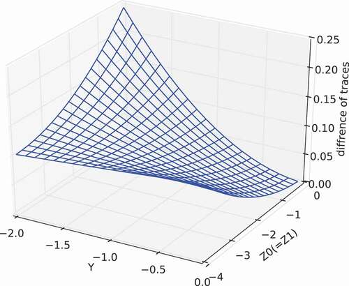
Moreover, Figures 1 and 2 show another calculation result of the difference of traces, namely $\mathrm{t}\mathrm{r}\left({\mathbf{M}}_{\mathrm{M}\mathrm{L}\mathrm{E}\mathrm{A}}^{\ast }\right)-\mathrm{t}\mathrm{r}\left({\mathbf{M}}_{\mathrm{M}\mathrm{L}\mathrm{E}\mathrm{A}}^{min}\right)$, for the simplified case. In this calculation, we defined by $\mathbf{Y}=y\mathbf{J}$ and ${\mathbf{Z}}_0={\mathbf{Z}}_1=z\mathbf{J}$, where $y$ and $z$ are scalar variables, and $\mathbf{J}$ represents the all-ones matrix, in which all elements are unity. Thus, by using $y$ and $z$, we changed $\mathbf{Y}$ and ${\mathbf{Z}}_0(={\mathbf{Z}}_1)$ around the zero matrix (i.e. around $y=z=0$). From these figure, we can see that the difference of traces becomes zero when $\mathbf{Y}=\mathbf{O}$ and ${\mathbf{Z}}_0=\mathbf{O}$ (i.e. ${\mathbf{G}}_0^{(2)-}={\mathbf{G}}^{(2)+}$). That is, $\mathrm{t}\mathrm{r}\left({\mathbf{M}}_{\mathrm{M}\mathrm{L}\mathrm{E}\mathrm{A}}^{min}\right)$ has the minimum value among $\mathrm{t}\mathrm{r}\left({\mathbf{M}}_{\mathrm{M}\mathrm{L}\mathrm{E}\mathrm{A}}^{\ast }\right)$.

Figure 1. Difference of the traces of ${\mathbf{M}}_{\mathrm{M}\mathrm{L}\mathrm{E}\mathrm{A}}^{\ast }$ and ${\mathbf{M}}_{\mathrm{M}\mathrm{L}\mathrm{E}\mathrm{A}}^{min}$ as a function of $\mathbf{Y}(=y\mathbf{J})$ and ${\mathbf{Z}}_0(={\mathbf{Z}}_1=z\mathbf{J})$ within the ranges of $0\le y\le 2$ and $0\le z\le 4$.

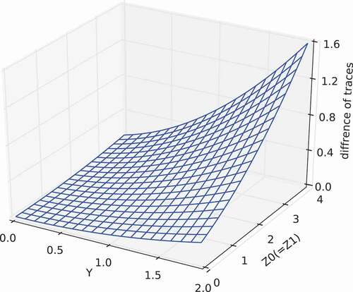
Figure 2. Difference of the traces of ${\mathbf{M}}_{\mathrm{M}\mathrm{L}\mathrm{E}\mathrm{A}}^{\ast }$ and ${\mathbf{M}}_{\mathrm{M}\mathrm{L}\mathrm{E}\mathrm{A}}^{min}$ as a function of $\mathbf{Y}(=y\mathbf{J})$ and ${\mathbf{Z}}_0(={\mathbf{Z}}_1=z\mathbf{J})$ within the ranges of $-2\le y\le 0$ and $-4\le z\le 0$.

4.4. Role of assumption of normal distribution

With regard to MLCA, it was found that the formulation equivalent to CBCA can be derived by introducing the assumption of linear estimation expressed by Equation (69)(69) $\hat{\mathbf{T}}-{\mathbf{T}}_0=\mathbf{F}\left({\mathbf{R}}_e^{(1)}-{\mathbf{R}}_c^{(1)}({\mathbf{T}}_0)\right).$(69) . Meanwhile, the same formula can be derived by using the other assumptions, that is, MSCA and DRCA. For this reason, we examine these assumptions necessary for deriving the formulation equivalent to CBCA. Table 1 summarizes the assumptions used in the derivation of CAs – including CBCA, MRCA, DRCA, MLCA, and MRCA.

Note that the assumption of normal distribution includes an assumption that the mean value is equal to the true value. Meanwhile, the mean value of the normal distribution is equal to the expectation value. Hence, we can understand that the assumption of normal distribution includes the assumption of unbiased estimation. Moreover, it should be noted that, when we assume the linear estimation of Equation (70)(70) ${\hat{\mathbf{R}}}^{(1)}-{\mathbf{R}}_c^{(1)}({\mathbf{T}}_0)=\mathbf{F}\left({\mathbf{R}}_e^{(1)}-{\mathbf{R}}_c^{(1)}({\mathbf{T}}_0)\right).$(70) , it is necessary to introduce the assumption of minimum norm solution:

(157) $\hat{\mathbf{T}}={\mathbf{T}}_0+{\mathbf{G}}^{(1)+}{\mathbf{F}}^{\prime }\left({\mathbf{R}}_e^{(1)}-{\mathbf{R}}_c^{(1)}({\mathbf{T}}_0)\right),$(157)

Table 1. Assumptions used in the derivation of the conventional cross-section adjustment methods

	CBCA	MSCA	DRCA	MLCA	MRCA
Normal distribution	✓
Unbiased estimation	(✓)${ }^{\ast }$	✓	✓	✓	✓
Linear estimation of Equation (70)(70) ${\hat{\mathbf{R}}}^{(1)}-{\mathbf{R}}_c^{(1)}({\mathbf{T}}_0)=\mathbf{F}\left({\mathbf{R}}_e^{(1)}-{\mathbf{R}}_c^{(1)}({\mathbf{T}}_0)\right).$(70)		✓	✓		✓
Minimum norm solution of Equation (157)(157) $\hat{\mathbf{T}}={\mathbf{T}}_0+{\mathbf{G}}^{(1)+}{\mathbf{F}}^{\prime }\left({\mathbf{R}}_e^{(1)}-{\mathbf{R}}_c^{(1)}({\mathbf{T}}_0)\right),$(157)		✓	✓		✓
Projection simplification		✓
Dimensionality reduction			✓
Linear estimation of Equation (69)(69) $\hat{\mathbf{T}}-{\mathbf{T}}_0=\mathbf{F}\left({\mathbf{R}}_e^{(1)}-{\mathbf{R}}_c^{(1)}({\mathbf{T}}_0)\right).$(69)				✓
Equivalence with the CBCA method	=	=	=	=	$\ne$

${ }^{\ast }$Included in the assumption of normal distribution

where ${\mathbf{F}}^{\prime }\in {\mathbb{R}}^{n^{(1)}\times n^{(1)}}$ is another linear combination factor (cf. Equation (40)(40) $\mathrm{E}\left({\mathbf{w}}_k{\mathbf{w}}_i^{\mathrm{T}}\right)=\left\{\begin{array}{c}{\mathbf{Q}}_k(i=k)\\ \mathbf{O}(i\ne k),\end{array}\right.$(40) in reference [9]). Note that the dimension of ${\mathbf{F}}^{\prime }$ differs from that of $\mathbf{F}$ used in the present derivation. We can see that both Equations (157)(157) $\hat{\mathbf{T}}={\mathbf{T}}_0+{\mathbf{G}}^{(1)+}{\mathbf{F}}^{\prime }\left({\mathbf{R}}_e^{(1)}-{\mathbf{R}}_c^{(1)}({\mathbf{T}}_0)\right),$(157) and (69(69) $\hat{\mathbf{T}}-{\mathbf{T}}_0=\mathbf{F}\left({\mathbf{R}}_e^{(1)}-{\mathbf{R}}_c^{(1)}({\mathbf{T}}_0)\right).$(69) ) include a concept of dimensionality expansion in the case that $n_a>n^{(1)}$: the former expands the dimension by ${\mathbf{G}}^{(1)+}\in {\mathbb{R}}^{n_a\times n^{(1)}}$, and the latter by $\mathbf{F}\in {\mathbb{R}}^{n_a\times n^{(1)}}$. Thus, we can deduce that either the projection simplification or the dimensionality reduction is required to compensate the dimensionality expansion introduced by the assumption of minimum norm solution.

Moreover, from this table, it is seen that the assumption of normal distribution adopted in CBCA is equivalent to a set of the assumptions of:

• unbiased estimation, linear estimation of Equation (70)(70) ${\hat{\mathbf{R}}}^{(1)}-{\mathbf{R}}_c^{(1)}({\mathbf{T}}_0)=\mathbf{F}\left({\mathbf{R}}_e^{(1)}-{\mathbf{R}}_c^{(1)}({\mathbf{T}}_0)\right).$(70) , minimum norm solution, and projection simplification.

• unbiased estimation, linear estimation of Equation (70)(70) ${\hat{\mathbf{R}}}^{(1)}-{\mathbf{R}}_c^{(1)}({\mathbf{T}}_0)=\mathbf{F}\left({\mathbf{R}}_e^{(1)}-{\mathbf{R}}_c^{(1)}({\mathbf{T}}_0)\right).$(70) , minimum norm solution, and dimensionality reduction.

• unbiased estimation and linear estimation of Equation (69)(69) $\hat{\mathbf{T}}-{\mathbf{T}}_0=\mathbf{F}\left({\mathbf{R}}_e^{(1)}-{\mathbf{R}}_c^{(1)}({\mathbf{T}}_0)\right).$(69) .

In summary, when we apply CBCA under the condition of the underdetermined problem, the assumption of normal distribution plays an important role to expand properly the information of the integral experimental quantities to the adjusted cross-section set.

4.5. Comparison with derivation based on Bayes theorem

From the derivations of MLCA, MLEA, MLRA, and MLEB, we can deduce that the assumptions of linear estimation expressed by Equations (69)(69) $\hat{\mathbf{T}}-{\mathbf{T}}_0=\mathbf{F}\left({\mathbf{R}}_e^{(1)}-{\mathbf{R}}_c^{(1)}({\mathbf{T}}_0)\right).$(69) –(71(71) ${\hat{\mathbf{R}}}^{(2)}-{\mathbf{R}}_c^{(2)}({\mathbf{T}}_0)=\mathbf{F}\left({\mathbf{R}}_e^{(1)}-{\mathbf{R}}_c^{(1)}({\mathbf{T}}_0)\right).$(71) ) correspond to conditional probabilities maximized in derivations based on the Bayes theorem:

(158) $P(\hat{\mathbf{T}}|{\mathbf{R}}_e^{(1)}),$(158)

(159) $P({\hat{\mathbf{R}}}^{(1)}|{\mathbf{R}}_e^{(1)}),$(159)

and

(160) $P({\hat{\mathbf{R}}}^{(2)}|{\mathbf{R}}_e^{(1)}),$(160)

respectively, where $P(\mathfrak{A}|\mathfrak{B})$ denotes the probability distribution of $\mathfrak{A}$ under the condition that $\mathfrak{B}$ is given. In fact, Equation (158)(158) $P(\hat{\mathbf{T}}|{\mathbf{R}}_e^{(1)}),$(158) is used explicitly in the derivation of CBCA [1,4], and Equation (160)(160) $P({\hat{\mathbf{R}}}^{(2)}|{\mathbf{R}}_e^{(1)}),$(160) is utilized in the derivation of CBEA [8] in the modified form:

(161) $P({\mathbf{R}}_c^{(2)}(\hat{\mathbf{T}})|{\mathbf{R}}_e^{(1)}).$(161)

Besides CBEA, a lot of new techniques based on the Bayes theorem have been recently proposed (e.g. [16–18]). Hence, a detailed comparison with these techniques would be a future task. The foregoing correspondence between the linear estimations and the conditional probabilities, however, will be useful for the comparison of our methodologies with the other techniques based on the Bayes theorem.

5. Conclusions

In comparison with the classical Bayesian conventional cross-section adjustment (CBCA) method, the derivation of the Kalman filter was reviewed. This review revealed that CBCA is equivalent to a linearized model of the nonlinear Kalman filter, while the assumption of linear estimation used in the cross-section adjustment methodology differs from that in the Kalman filter. For this reason, by introducing the assumption used in the Kalman filter, we formulated the conventional, extended, and regressive cross-section adjustment methods (CA, EA, and RA) with no use of the assumption of normal distribution; these methods are called the conventional, extended, and regressive cross-section adjustment methods based on minimum variance unbiased linear estimation (MLCA, MLEA, and MLRA), respectively. Consequently, we found that MLCA has the formulation equivalent to CBCA. From these findings, we discussed the role of the assumption of normal distribution adopted in CBCA. Moreover, we demonstrated that the extended bias factor (EB) method can be formulated with the same procedure; this method is referred to as MLEB. The derivation of MLEB is simple, and would be helpful to understand the difference between EB and EA.

With regard to MLEA, we derived a generalized formulation that can express all the numerous solutions minimizing the variance of the design target core parameters. The formulation of MLEA includes a special case identical to the conventional Bayesian extended cross-section adjustment (CBEA) method; when we adopt the special case, the variance of adjusted cross-section set is also minimized. Thus, we can interpret that CBEA minimizes not only the variance of the design target core parameters but also the variance of the nuclear data. For this reason, we recommend to use the special case of MLEA, which is equivalent to CBEA, from a practical point of view.

On the other hand, in our review, we showed that CBCA is a type of the Kalman filter. Since many enhanced techniques based on the Kalman filter have been proposed in the other fields, we expect that an application of these techniques lead to further improvement in the cross-section adjustment methodology. Moreover, MLEA itself is an enhancement of the Kalman filter. Therefore, MLEA would be applicable in various fields other than nuclear reactor design.

Abbreviations

1. derivation procedures

   CB : classical Bayesian (inference)

   MVUE : minimum variance unbiased estimation

   MVULE : minimum variance unbiased linear estimation

2. variations of cross-section adjustment methodology

   CA : conventional cross-section adjustment method

   EA : extended cross-section adjustment method

   RA : regressive cross-section adjustment method

3. CAs

   CBCA : classical Bayesian conventional cross-section adjustment method

   MRCA : MVUE-based rigorous conventional cross-section adjustment method

   MSCA : MVUE-based simplified conventional cross-section adjustment method

   MLCA : MVULE-based conventional cross-section adjustment method

   DRCA : dimension-reduced conventional cross-section adjustment method

4. EAs

   CBEA : classical Bayesian extended cross-section adjustment method

   MREA : MVUE-based rigorous extended cross-section adjustment method

   MSEA : MVUE-based simplified extended cross-section adjustment method

   MLEA : MVULE-based extended cross-section adjustment method

5. RA

   MLRA : MVULE-based regressive cross-section adjustment method

6. extended bias factor methods

   EB : (original) extended bias factor method

   MLEB : MVULE-based extended bias factor method

Acknowledgments

The authors express their deep gratitude to the coauthors of references [8–10], since the present study is due to discussion with them through the series of studies. The authors are also grateful to Dr S. Takeda of Osaka University for useful comments on the present study. K. Yokoyama wishes to extend his special thanks to Mr M. Ishikawa of JAEA for great encouragement and helpful discussion based on his expertise.

Disclosure statement

No potential conflict of interest was reported by the authors.

References

- Dragt JB. Statistical considerations on techniques for adjustment of Differential cross sections with measured integral parameters. In: STEK, The fast-thermal coupled facility of RCN at Petten. RCN-122. Petten: Reactor Centrum Nederland; 1970. p. 85–105.
- Gandini A, Petilli M, Salvatores M. Nuclear data and integral measurement correlation for fast reactors. Statistical formulation and analysis of methods. The Consistent Approach. International Symposium of Physics of Fast Reactors, 1973 October 16-19. Tokyo, Japan; Vol. 1. p. 612–628.
- Dragt JB, Dekker JWM, Guppelaar H, et al. Methods of adjustment and error evaluation of neutron capture cross sections; Application to fission product nuclides. Nucl Sci Eng. 1977;62:117–129.
- Takeda T, Yoshimura A, Kamei T. Prediction uncertainty evaluation methods of core performance parameters in large liquid-metal fast breeder reactors. Nucl Sci Eng. 1989;103:157–165.
- Salvatores M, Palmiotti G, Aliberti G, et al. Methods and issues for the combined use of integral experiments and covariance data: results of a NEA International Collaborative Study. Nuclear Data Sheets. 2014;118:38–71.
- de Saint-Jean C, Dupont E, Ishikawa M, et al. Assessment of existing nuclear data adjustment methodologies. Paris: OECD/NEA; 2011. NEA/NSC/WPEC/DOC(2010)429.
- Kugo T, Mori T, Takeda T. Theoretical study on new bias factor methods to effectively use critical experiments for improvement of prediction accuracy of neutronic characteristics. J Nucl Sci Technol. 2007;44(12):1509–1517.
- Yokoyama K, Ishikawa M, Kugo T. Extended cross-section adjustment method to improve the prediction accuracy of core parameters. J Nucl Sci Technol. 2012;49(12):1165–1174.
- Yokoyama K, Yamamoto A. Cross-section adjustment methods based on minimum variance unbiased estimation. J Nucl Sci Technol. 2016;53(10):1622–1638.
- Yokoyama K, Yamamoto A, Kitada T. Dimension-reduced cross-section adjustment methods based on minimum variance unbiased estimation. J Nucl Sci Technol. 2018;55(3):319–334.
- Kalman RE, New A. Approach to linear filtering and prediction problems. Trans ASME J Basic Eng. 1960;82:35–45.
- Kalman RE, Bucy RS. New results in linear filtering and prediction therory. Trans ASME J Basic Eng. 1961;83:95–108.
- Harville DA. Matrix algebra from a statistician’s perspective. 1st ed. New York (NY): Springer; 1997.
- Brown RG, Hwang PYC. Introduction to random signals and applied Kalman filtering. 4th ed. Hoboken (NJ): John Wiley & Sons, Inc; 2012.
- Palmiotti G, Salvatores M, Yokoyama K, et al. Methods and approaches to provide feedback from nuclear and covariance data adjustment for improvement of nuclear data files. Paris: OECD/NEA; 2017. NEA/NSC/WPEC/DOC(2016)6.
- Cacuci DG, Ionescu-Bujor M. Best-estimate model Calibration and Prediction Through Experimental Data Assimilation – I: mathematical Framework. Nucl Sci Eng. 2010;165:18–44.
- Hoefer A, Buss O, Hennebach M, et al. MOCABA: A general Monte Carlo-Bayes pro- cedure for improved predictions of integral functions of nuclear data. Ann Nucl Energy. 2015;77:514–521.
- Endo T, Yamamoto A, Watanabe T. Bias factor method using random sampling technique. J Nucl Sci Technol. 2016;53:1494–1501.