Visualized measurement of extremely high-speed droplets in Venturi scrubber

ABSTRACT

Venturi scrubbers for filtered venting have been installed in nuclear power plants worldwide. Venturi scrubbers can eliminate fission products from a polluted gas by interaction through gas–liquid interfaces. Therefore, droplet diameter is important from the viewpoint of decontamination. When Venturi scrubbers are used in severe accidents, the gas flow velocity might be extremely high. In these studies, the authors did not measure droplet diameter under extremely high gas velocity conditions. In the scenarios, experimental data pertaining to droplet diameter, under the extremely high gas flow velocity, are required. Therefore, this objective is to evaluate the diameter of extremely high-speed droplets. A visualization experiment was conducted using a Venturi scrubber. The droplet diameter distribution and the Sauter mean diameter (SMD) were determined. By comparing between the experimental value of SMDs and the one evaluated using Nukiyama–Tanasawa equation, it was confirmed that the Nukiyama–Tanasawa equation can be used to evaluate SMD with good accuracy in the gas velocity range of 82–250 m/s, except the highest gas velocity conditions. Furthermore, the droplet generation mechanism in the Venturi scrubber was considered to clarify the main reason why the Nukiyama–Tanasawa equation can be used to evaluate SMD droplet diameter.

KEYWORDS:

• Venturi scrubber
• filtered venting
• self-priming
• self-priming suspension
• annular dispersed flow
• droplet generation
• visualization

1. Introduction

In nuclear power plants in Japan, filtered venting systems have been installed to prevent environmental contamination by radioactive fission products of severe accidents. The main component of one such filtered venting system is a Venturi scrubber. During filtered venting, a dispersed or an annular dispersed flow including microscale droplets is formed [1–5] in the Venturi scrubber, and it decontaminates particulate and gaseous fission products in the pollutant gas [1–4]. The maximum gas velocity at the throat part of the Venturi scrubber has been evaluated to reach 120 m/s [6]. Therefore, inertial impaction between the aerosol particles and the droplets in the flow and absorption of the gaseous fission products into the droplets are considered the main decontamination mechanisms [2,3,6,7]. In view of these mechanisms, the following equations to evaluate decontamination performance were proposed by Ali et al. [3,7].

(1) $E_{\mathrm{A}\mathrm{e}\mathrm{r}\mathrm{o}\mathrm{s}\mathrm{o}\mathrm{l}\mathrm{p}\mathrm{a}\mathrm{r}\mathrm{t}\mathrm{i}\mathrm{c}\mathrm{l}\mathrm{e}\mathrm{s}}=1-\frac{C_{\mathrm{o}\mathrm{u}\mathrm{t}}}{C_{\mathrm{i}\mathrm{n}}}=1-exp\left(-\frac{3}{2}\frac{Q_{\mathrm{L}}}{Q_{\mathrm{G}}}\frac{x}{D_{\mathrm{d}}^2}\frac{u_{\mathrm{d}}}{\left|u_{\mathrm{G}}-u_{\mathrm{d}}\right|}\eta \right)$(1)

(2) $\eta ={\left(\frac{\psi }{\psi +0.7}\right)}^2$(2)

(3) $\psi =\frac{{\rho }_{\mathrm{p}}{D}_{\mathrm{p}}^2\left(u_{\mathrm{p}}-u_{\mathrm{d}}\right)}{9{\mu }_{\mathrm{G}}{D}_{\mathrm{d}}}$(3)

(4) $E_{\mathrm{G}\mathrm{a}\mathrm{s}\mathrm{e}\mathrm{o}\mathrm{u}\mathrm{s}\mathrm{i}\mathrm{o}\mathrm{d}\mathrm{i}\mathrm{n}\mathrm{e}}=1-\frac{C_{\mathrm{o}\mathrm{u}\mathrm{t}}}{C_{\mathrm{i}\mathrm{n}}}=1-exp\left(-\frac{4\pi D_{\mathrm{d}}^2{k}_{\mathrm{G}}}{V_{\mathrm{d}}}t\right)$(4)

In these equations, C_in and C_out [kg/m³] are the mass concentrations of fission products at the inlet and the outlet, respectively. D_d and D_p [m] are droplet and particle diameters, respectively. E_{Aerosol particles} and E_{Gaseous iodine} [−] are removal efficiencies for aerosol particles and gaseous iodine, respectively. k_G [m] is a gas-side mass transfer coefficient; Q_G [m³/s] and Q_L are the volumetric flow rate of gas and total droplets, respectively. u_d, u_G, and u_p [m/s] are the velocities of droplets, gas, and particles, respectively. η is impaction efficiency, μ_G is a gas viscosity coefficient, ρ_p is particle density, and ψ is inertial coefficient. $V_{\mathrm{d}}=\pi D_{\mathrm{d}}^3/6$ [m³] is the volume of a single droplet.

In the above equations, droplet diameter D_d is one of the important parameters to be evaluated. To evaluate droplet diameter in a dispersed flow, the Nukiyama–Tanasawa equation [8–11] is often used. The equation is as follows.

(5) $D_{\mathrm{d}32}=\frac{585\times {10}^{-9}}{\left|u_{\mathrm{G}}-u_{\mathrm{L}}\right|}{\left(\frac{\sigma }{{\rho }_{\mathrm{L}}}\right)}^{0.5}+211.8\times {10}^{-6}{\left(\frac{{\mu }_{\mathrm{L}}}{\sqrt{\sigma {\rho }_{\mathrm{L}}}}\right)}^{0.45}{\left(1000\frac{Q_{\mathrm{L}}}{Q_{\mathrm{G}}}\right)}^{1.5}$(5)

In this equation, D_d32 [m] is the Sauter mean diameter (SMD) of droplets, and σ [N/m] is surface tension. Notably, the experimental coefficients, 585 × 10⁻⁹ and 211.8 × 10⁻⁶, are not non-dimensional values, but they are values converted from the original values based on the CGS system of units to those based on the SI units. Equation (5)(5) $D_{\mathrm{d}32}=\frac{585\times {10}^{-9}}{\left|u_{\mathrm{G}}-u_{\mathrm{L}}\right|}{\left(\frac{\sigma }{{\rho }_{\mathrm{L}}}\right)}^{0.5}+211.8\times {10}^{-6}{\left(\frac{{\mu }_{\mathrm{L}}}{\sqrt{\sigma {\rho }_{\mathrm{L}}}}\right)}^{0.45}{\left(1000\frac{Q_{\mathrm{L}}}{Q_{\mathrm{G}}}\right)}^{1.5}$(5) was derived based on experimental studies conducted using spray nozzles, and these experimental studies were performed under the following conditions: 0.8 × 10³ < ρ_L < 1.2 × 10³ [kg/m³], 30 × 10⁻³ < σ < 73 × 10⁻³ [N/m], 0.01 × 10⁻¹ < μ_L < 0.25 × 10⁻¹ [kg/(m∙s)], 100 < u_G < 300 [m/s], 1 × 10³ < Q_G/Q_L < 10 × 10³.

A Venturi scrubber is a Venturi pipe with small holes in the throat part. Surrounding liquid is sucked in through these small holes, and small droplets are generated (atomization) in the throat part [6] owing to velocity differences between the gas and the liquid in question. This droplet generation mechanism owing to the velocity difference is the almost same as that of the spray nozzles used in the experiments to develop Equation (5)(5) $D_{\mathrm{d}32}=\frac{585\times {10}^{-9}}{\left|u_{\mathrm{G}}-u_{\mathrm{L}}\right|}{\left(\frac{\sigma }{{\rho }_{\mathrm{L}}}\right)}^{0.5}+211.8\times {10}^{-6}{\left(\frac{{\mu }_{\mathrm{L}}}{\sqrt{\sigma {\rho }_{\mathrm{L}}}}\right)}^{0.45}{\left(1000\frac{Q_{\mathrm{L}}}{Q_{\mathrm{G}}}\right)}^{1.5}$(5) . Therefore, this equation is often used to evaluate droplet diameter generated in Venturi scrubbers [2,3,6].

The applicability of Equation (5)(5) $D_{\mathrm{d}32}=\frac{585\times {10}^{-9}}{\left|u_{\mathrm{G}}-u_{\mathrm{L}}\right|}{\left(\frac{\sigma }{{\rho }_{\mathrm{L}}}\right)}^{0.5}+211.8\times {10}^{-6}{\left(\frac{{\mu }_{\mathrm{L}}}{\sqrt{\sigma {\rho }_{\mathrm{L}}}}\right)}^{0.45}{\left(1000\frac{Q_{\mathrm{L}}}{Q_{\mathrm{G}}}\right)}^{1.5}$(5) to Venturi scrubbers was validated by Guerra et al. [12], who considered gas velocities lower than 70 m/s in the throat part. However, for gas velocities higher than 120 m/s, the applicability of this equation has not been confirmed. The gas velocity in the Venturi scrubber depends strongly on its geometry and the working conditions. It was suggested that depending on the progression of an accident, the gas velocity in the throat part may exceed 120 m/s [2,13].

To precisely evaluate the decontamination performance during filtered venting, the equation for calculating droplet diameter must be validated under high gas velocity conditions. To perform validation works, measured droplet diameter data under high gas velocity conditions are required, but it is very difficult to measure droplet diameter under high gas velocity conditions because the droplets are very small and very fast to measure by general method.

In this study, we developed a method based on visualization and image processing to measure droplet diameter under extremely high speeds. Droplet diameters in the Venturi scrubber were measured over a wide range of gas velocity, and by using the measured data, a few equations for calculating droplet diameter were validated. In addition, the droplet generation mechanism was discussed based on the observed hydraulic behaviors and droplet diameters in the Venturi scrubber.

2. Experimental method

2.1. Experimental apparatus and procedure

The experimental apparatus used in this study was almost the same as that used in the previous study [14], except that a visualization vessel was added downstream of the test section. An outline of this apparatus is shown in Figure 1. The apparatus was composed of a Venturi scrubber as the test section, an air feed system with two compressors, an overflow tank, and a visualization vessel. The visualization vessel was made of acrylic, and it measured 300 mm in width, 300 mm in depth, and 600 mm in height. The top of the visualization vessel was open, and this vessel was installed to eliminate the effect of liquid films on droplet visualization, as well as to prevent water scattering. The fluids, air and water, were exposed to the atmosphere through this vessel. The Venturi scrubber geometry was the same as that in the previous study [15], and the cross-section of the throat part was 20.0 mm², cross sections of the inlet and the outlet were 84.8 mm², and diameter of the hole for suction was 1 mm.

Figure 1. Experimental apparatus.

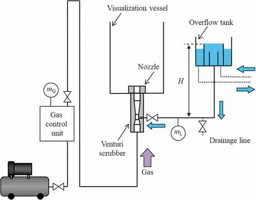
The experimental procedure was as follows. Firstly, the overflow tank was filled with supplied water, and the hydraulic head pressure to the hole was maintained at a constant value. Next, air flow was introduced into the Venturi scrubber section from the compressors, and a valve between the overflow tank and the hole was opened. If pressure in the throat part was lower than the water pressure in the hole, water flowed into the Venturi scrubber, and air and water formed a dispersed or an annular dispersed flow in the Venturi scrubber, and they were exposed to the visualization vessel. This water supply based on pressure difference between the gas and the liquid is called ‘self-priming.’ The mass flow rates of gas and liquid were measured using mass flow meters for both fluids, as shown in Figure 1, and superficial velocities in the throat part of the Venturi scrubber were calculated: $j=\dot{m}/\left({\rho }_{\mathrm{\infty }}\cdot A\right)$. In this equation, $A$ [m²] is the cross-sectional area. $j$ [m/s] is the superficial gas velocity. $\dot{m}$ [kg/s] is the measured gas mass flow rate. ${\rho }_{\mathrm{\infty }}$ [kg/m³] is the gas density at atmospheric pressure, ${\rho }_{\mathrm{\infty }}=1.165$ kg/m³. Superficial gas velocity using the gas density at atmospheric pressure can be used as a parameter to understand hydraulic behavior in Venturi scrubbers was confirmed [14]. In this paper, superficial gas velocity is used as a parameter to study about droplet diameter of Venturi scrubber to be expected close relation to the hydraulic behavior.

The experimental condition was essentially the same as that employed by Horiguchi et al. [14]. The distance from the water surface in the overflow tank to the suction hole was 1,000 mm. Superficial gas and liquid velocities in the throat part ranged from 83 to 292 m/s and 0 to 69 mm/s, respectively. Over the gas velocity range, visualization was not possible because a suspension was formed owing to self-priming, and droplet generation stopped.

2.2. Visualization method

2.2.1. Components of optical system

As the first step, we tried to visualize the droplets to measure the droplet diameter by using a combination of a high-speed video camera and a camera lens with a general working distance of 50 or 100 mm. However, the droplets could not be visualized on the snapshots because they were very small and very fast. Therefore, we increased the resolution of each snapshot and the working distance, and decreased the exposure time of the optical system.

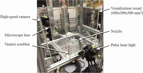
The improved optical system was composed of a high-speed video camera, microscope lens, and short pulse laser light. Figure 2 shows their positional relationship with the experimental apparatus. The microscope lens helped increase the system resolution, and the laser helped reduce the exposure time. A FASTCAM Mini UX100 (Fotron Ltd.), Leica Z16 APO (Leica Microsystems GmbH), and CAVILUX Smart (Cavitar Ltd.) were used as the high-speed camera, microscope lens, and pulse laser light, respectively. The short-pulse laser was set across the visualization vessel from the camera to serve as a backlight. The wavelength of the laser was approximately 810 nm, frame rate was 20,000, and exposure time was 20 ns. The setup method for the exposure time is explained in 2.2.3.

Figure 2. Positional relationship of experimental apparatus and optical system.

2.2.2. Method of visualization experiment

An original image and a processed image are shown in Figure 3 as examples of images obtained using the developed measurement method. The size and position of the visualized area are shown in Figure 3 as well. The visualized area was on the central axis and over the outlet of the Venturi scrubber, and the distance between the outlet and the central point of the visualized area was 4 mm. The visualized area measured 2.11 mm in height, 4.06 mm in width, and 50 μm in depth, and its resolution was about 4 μm/pixel.

Figure 3. Position of visualized area according to proposed measurement method.

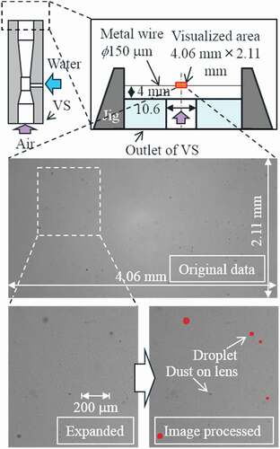
The droplets generated in the Venturi scrubber were visualized on the area, and the diameter of each droplet was determined from the snapshots by image processing. The visualization procedure, which is the first step in the developed method, is as follows. Before the experiment started, a metal wire with a diameter of 150 μm, as in Figure 3, was set over the outlet of the Venturi scrubber to pass through the central point of the visualized area. The optical system was adjusted to visualize the wire and the droplets clearly in a preliminary experiment. The wire was used as a measure to determine the resolution of the snapshot images. Then, the wire was moved out of the visualized area, a snapshot was taken as a background image for the image processing, and the experiment was started.

For visualization of a droplet in mist, elimination of other droplets overlapping with the target droplet is essential. To this end, we used a microscope lens with a thin depth of field to eliminate the unnecessary droplets by defocusing. Based on preliminary visualization, the largest number of droplets under a few experimental conditions seemed to have a diameter of be approximately 20 μm. Accordingly, the depth of field, approximately 50 μm, was defined as two to three times larger than the aforementioned diameter.

Also, based on preliminary visualization, the size of the visualized area was determined to ensure that an adequate number of droplets could be analyzed to understand the trend of droplet diameter, as in Figures 7 and 8, and to ensure that the size is as large as the resolution permits.

Figure 4. Exposure time setup.

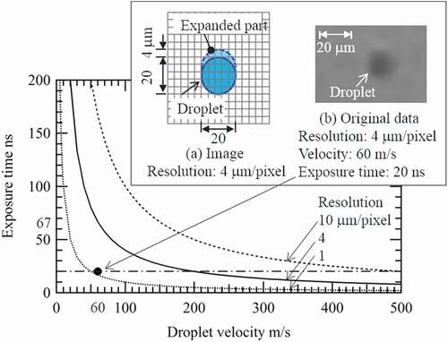
Figure 5. Series of snapshots obtained using proposed image processing scheme.

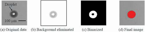
Figure 6. Relationship among gas velocity, liquid velocity, and liquid-gas ratio.

Figure 7. Superimposed images of droplets measured in 100 snapshots at superficial gas velocities of 83–292 m/s.

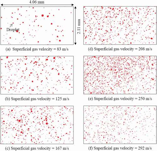
Figure 8. Droplet diameter distributions at superficial gas velocities of 83–292 m/s.

2.2.3. Exposure time to obtain clear images for measuring droplet size

The exposure time of the short-pulse laser is important for obtaining a clear image of the droplet. If the exposure time is long, the obtained droplet image is stretched out and hazy. If the exposure time is short, the amount of light available is small, and an image of the droplet cannot be obtained.

To compute the maximum exposure time, the relationship between the allowable stretching length and the maximum droplet velocity in the visualization area was considered. The maximum exposure time $\mathrm{\Delta }{t}_{\mathrm{e}\mathrm{x}}$ [s] was calculated as $\mathrm{\Delta }{t}_{ex}=\mathrm{\Delta }l/u_{\mathrm{d}}$. $\mathrm{\Delta }l$ [m] is the allowable stretching length of the droplet as the short pulse laser flashes, and $u_d$ [m/s] is the droplet velocity. In the experiment, the maximum velocity at the Venturi scrubber outlet was approximately 70 m/s based on the inlet mass flow rate. The droplet velocity was considered almost equal to the gas velocity, but there was the possibility of that a few droplets could have higher velocities. Then, we set the droplet velocity to 100 m/s to account for fluctuations in droplet velocity. Based on the performance of the microscope lens and the high-speed camera, as well as the results of preliminary visualization, we defined half the resolution of the high-speed video camera (4 μm/pixel) as the allowable stretching length of the droplet, and $\mathrm{\Delta }{t}_{ex}$ = 20 ns. Figure 4 shows the relationship between the maximum exposure time and droplet velocity. In Figure 4, the horizontal line represents droplet velocity, and the vertical line represents exposure time. Finally, we set 20 ns as the exposure time and performed visualization; an example of the obtained images is shown in Figure 4(b). A droplet measuring approximately 20 μm in diameter was visualized without expansion, and we confirmed that we could visualize small high-velocity droplets by using the developed optical system.

2.3. Image processing method

As the second step in the measurement of droplet diameters, the following image processing method was applied to the obtained snapshot images of droplets. Background elimination, binarization at the threshold level, and outline extraction were conducted, as shown in Figure 5, and projected areas of the droplets were obtained. Then, the droplet diameters were calculated as equivalent diameters from these areas. Figure 5 shows the flow of the image processing scheme employed herein, for example, (a) shows the original data, which represents a sample droplet, (b) shows the background-eliminated data, (c) shows binarized data, and (d) shows the data after outline extraction, obtained by drawing the outline and filling it in on the original data. The outline of the sample droplet in Figure 5 was seemingly recognized precisely.

By means of background elimination and binarization, we eliminated unnecessary objects, dust on the lens, and defocused droplets. For binarization, we determined the threshold level by comparing several droplet diameters obtained by image processing to ones obtained by visual measurement. The threshold level was changed as a parameter, and selected to fit the diameters of the image processing to the ones of the visual measurement with the best accuracy. In the visual measurement, droplet diameter was obtained as equivalent area diameter from the original data by counting the number of pixels constituting the droplet and calculating the equivalent diameter in the area.

The accuracy of image processing in terms of relative error is summarized, and the details of a few of the droplets measured using the two methods, namely, visual measurement and image processing, are summarized as examples in Table 1. The relative error [%] between the visual measurement and the image processing was calculated using the following equation.

(6) $\mathrm{R}\mathrm{e}\mathrm{l}\mathrm{a}\mathrm{t}\mathrm{i}\mathrm{v}\mathrm{e}\mathrm{e}\mathrm{r}\mathrm{r}\mathrm{o}\mathrm{r}=\frac{D_{\mathrm{d}\mathrm{I}\mathrm{P}}-D_{\mathrm{d}\mathrm{V}\mathrm{M}}}{D_{\mathrm{d}\mathrm{V}\mathrm{M}}}\times 100$(6)

Table 1. Relative error

Measured μm	Image processed μm	Relative error %
10	9.73	−6.00
13	10.26	−19.10
16	16.22	4.44
28	38.79	39.16
28	41.28	45.62
29	46.21	60.36
32	32.43	0.35
36	34.02	−5.14
37	36.26	−0.92
49	48.33	−2.12
52	42.78	−17.34
60	82.25	37.79
91	88.53	−2.22
243	244.96	0.88
Average of relative error, %		9.70
Standard deviation of relative error, %		24.09

In equation (6)(6) $\mathrm{R}\mathrm{e}\mathrm{l}\mathrm{a}\mathrm{t}\mathrm{i}\mathrm{v}\mathrm{e}\mathrm{e}\mathrm{r}\mathrm{r}\mathrm{o}\mathrm{r}=\frac{D_{\mathrm{d}\mathrm{I}\mathrm{P}}-D_{\mathrm{d}\mathrm{V}\mathrm{M}}}{D_{\mathrm{d}\mathrm{V}\mathrm{M}}}\times 100$(6) , D_dIP [m] and D_dVM [−] denote the droplet diameters determined by image processing and visual measurement, respectively. The average relative error was 9.70%, and the standard deviation σ₀ was 24.09%. Therefore, the visually measured value ranged from −14.4 to 33.8% of the image-processed value with a probability of 1 σ₀. In Table 1, a few of the relative errors are high, even up to 60%.

Furthermore, the theoretical maximum relative error between a real droplet and a droplet comprised of pixels, like the ones on the snapshots, can be calculated as follows. There is a droplet, of diameter 2r and projected area Πr², and four pixels, wherein the side length of each pixel is r and the total area is 4r². The unit of r is [m]. When the droplet is visualized on the four pixels, it is observed as a box composed of the four pixels on the snapshot because of the resolution, and its area is calculated as 4r² in the image processing. On a side note, four pixels are minimum to visualize a droplet because that the diameter of a smaller droplet than a pixel can not to be measured. So, the theoretical maximum relative error is 27.3%.

By comparing the values of the average relative error and the range via the theoretical maximum relative error, the image processing had a sufficient accuracy was concluded, but a few of the relative errors in Table 1 are higher than the theoretical one. That possible reason is the accuracy of the rejection of the defocused droplet in the method of image processing. A few droplets were visualized with low difference in brightness between the droplet and the background because of the defocusing. Some defocused droplets were rejected during image processing, but the other droplets were retained with revised outlines. Therefore, it is plausible for these droplets to be characterized by high relative errors. Based on this result, the SMD considering errors was computed using the following equation.

(7) $D_{\mathrm{d}32}\pm {\delta }_{D_{\mathrm{d}32}}=\frac{\sum \left\{{\left(D_{\mathrm{d}i}\pm {\delta }_{D_{\mathrm{d}i}}\right)}^3\mathrm{\Delta }{n}_i\right\}}{\sum \left\{{\left(D_{\mathrm{d}i}\pm {\delta }_{D_{\mathrm{d}i}}\right)}^2\mathrm{\Delta }{n}_i\right\}}$(7)

where D_d32 [m] is the SMD, D_di [m] is the droplet diameter in Section i, δ [m] is the error in droplet diameter, and Δn_i is the number of droplets in Section I. −δ _Ddi is −0.144D_di, and +δ _Ddi is 0.338 D_di.

3. Result and discussion

3.1. Measurement and evaluation results of self-priming as the basis of droplet evaluation

The liquid–gas ratio is thought to influence the tendency of SMD. In a self-priming Venturi scrubber, the liquid flow rate changes in accordance with the gas flow rate.

Then, in terms of the basic data related to SMD, the gas and liquid flow rate were measured experimentally. In addition, the superficial gas and liquid velocities in the throat part and the liquid–gas ratio, $Q_{\mathrm{L}}/Q_{\mathrm{G}}$, were computed using the obtained data. Figure 6 shows the relationship among the superficial gas velocity, superficial liquid velocity, and liquid-gas ratio in the throat part of the Venturi scrubber. In Figure 6, the horizontal axis represents the superficial gas velocity. The left vertical axis represents the superficial liquid velocity, and the right vertical axis represents the liquid-gas ratio. Open circle plots and open rectangular plots denote the evaluated values of superficial liquid velocity and liquid-gas ratio, respectively. The measurement and evaluation errors therein are shown in Figure 6, but most of them are very small. In terms of the relationship between the gas velocity and the liquid velocity, the superficial liquid velocity was approximately 50 mm/s at zero superficial gas velocity, and it reached its maximum value when the superficial gas velocity was approximately $j_g=$150 m/s owing to a decrease in pressure in the throat part. For $j_g>$150 m/s, the superficial liquid velocity decreased to 0 mm/s. This means the self-priming is suspended when the superficial gas velocity reaches a certain value. This result is consistent with the result of a previous report [14]. In Figure 6, the liquid–gas ratio immediately decreased two-fold with increasing superficial gas velocity. This decrease was caused by the change of the superficial liquid velocity.

3.2. Measurement and evaluation results of droplet diameter

The droplet diameters were obtained using the measurement method explained in Section 2. Figure 7 shows examples of the processed final images. In Figure 7, the droplets in 100 snapshots were superimposed on one picture for each superficial gas velocity. At the superficial gas velocity of 83 m/s, the diameters of a few droplets exceeded 100 μm. The droplet diameter decreased and the number of droplets increased as the superficial gas velocity increased until 250 m/s. At the superficial gas velocity of 292 m/s, droplet size seemed to be the same as that at 250 m/s, but the number of droplets was smaller than that at 250 m/s.

Figure 8 shows droplet diameter distributions based on the measurement results. The horizontal axis represents droplet diameter. The left vertical axis represents the probability distribution function (PDF), and the right vertical axis represents the cumulative distribution function (CDF) of the number of droplets. Histograms denote the PDFs obtained in the experiment, and open-circle plots denote the CDFs obtained in the experiment. The solid lines denote the gamma distributions used to evaluate the histograms. The width of a histogram bar is 6 μm.

In the PDF, the droplet diameters were smaller than 100 μm, except at the superficial gas velocity of 83 m/s. The histogram peak increased from 0.17 to 0.34 with increasing superficial gas velocity. The number of smaller droplets increased and that of larger droplets decreased, which was consistent with the trend shown in Figure 7. In the CDF, droplet diameters decreased when the CDFs reached 0.99 with increasing superficial gas velocity. This tendency was consistent with one of the histogram peaks in the PDF. Therefore, we obtained the data of high-velocity droplets in the Venturi scrubber to understand the tendency of change in droplet diameter.

To estimate the droplet diameter distribution, we considered the use of a distribution function. In general, a droplet diameter distribution is biased toward smaller size, and it can be represented using the gamma distribution [10] as follows.

(8) $\frac{\mathrm{\Delta }{n}_i}{N}=\frac{{\lambda }^m}{\mathrm{\Gamma }\left(m\right)}{\left(\frac{D_{\mathrm{d}i}}{D_{\mathrm{d}10}}\right)}^{m-1}exp\left(-\lambda \frac{D_{\mathrm{d}}}{D_{\mathrm{d}10}}\right)\frac{\mathrm{\Delta }{D}_{\mathrm{d}i}}{D_{\mathrm{d}10}}$(8)

In equation (8)(8) $\frac{\mathrm{\Delta }{n}_i}{N}=\frac{{\lambda }^m}{\mathrm{\Gamma }\left(m\right)}{\left(\frac{D_{\mathrm{d}i}}{D_{\mathrm{d}10}}\right)}^{m-1}exp\left(-\lambda \frac{D_{\mathrm{d}}}{D_{\mathrm{d}10}}\right)\frac{\mathrm{\Delta }{D}_{\mathrm{d}i}}{D_{\mathrm{d}10}}$(8) , D_di [m] is a droplet in section I; ΔD_di [m] is the measurement range of number of droplets, which is counted as -ΔD_d/2 ~ + ΔD_d/2; D_d10 [m] is arithmetic mean diameter; m is a function of σ₀, m = 1/σ₀²; N is the total number of droplets; Δn is the number of droplets in the range of -ΔD_d/2 ~ + ΔD_d/2; Γ (m) is the gamma function as a function of m; λ is a function of m, λ = m; and σ₀ is the standard deviation of the gamma distribution.

In Figure 8, the gamma distributions are fitted to the histograms. Constant numbers of the gamma distribution in Equation (8)(8) $\frac{\mathrm{\Delta }{n}_i}{N}=\frac{{\lambda }^m}{\mathrm{\Gamma }\left(m\right)}{\left(\frac{D_{\mathrm{d}i}}{D_{\mathrm{d}10}}\right)}^{m-1}exp\left(-\lambda \frac{D_{\mathrm{d}}}{D_{\mathrm{d}10}}\right)\frac{\mathrm{\Delta }{D}_{\mathrm{d}i}}{D_{\mathrm{d}10}}$(8) are listed in Table 2. The constant numbers range from 27.7 to 14.1 as the arithmetic mean diameter and from 0.80 to 0.59 as the standard deviation of the distribution. These numbers tended to decrease with increasing superficial gas velocity. The good fit seen in the results indicated that the gamma distribution can represent the droplet diameter distribution of the Venturi scrubber used for filtered venting. The applicable range of superficial gas velocity in the throat part of the Venturi scrubber was 89–292 m/s.

Table 2. Constant values in gamma distribution (Equation (8)(8) $\frac{\mathrm{\Delta }{n}_i}{N}=\frac{{\lambda }^m}{\mathrm{\Gamma }\left(m\right)}{\left(\frac{D_{\mathrm{d}i}}{D_{\mathrm{d}10}}\right)}^{m-1}exp\left(-\lambda \frac{D_{\mathrm{d}}}{D_{\mathrm{d}10}}\right)\frac{\mathrm{\Delta }{D}_{\mathrm{d}i}}{D_{\mathrm{d}10}}$(8) )

Superficial gas velocity in throat part [m/s]	83	125	167	208	250	292
Arithmetic mean diameter D10 [μm]	27.7	22.6	18.7	16.6	14.4	14.1
Standard deviation of gamma distribution σ0	0.80	0.65	0.66	0.65	0.59	0.59

3.3. Evaluation and comparison results of SMD

To statistically represent the characteristics of droplet size, SMD is often used because the relationship between the volumes and the surface areas of the droplets is important in terms of the decontamination mechanism. Figure 9 shows the SMD calculated from the experimental distribution by using Equation (7)(7) $D_{\mathrm{d}32}\pm {\delta }_{D_{\mathrm{d}32}}=\frac{\sum \left\{{\left(D_{\mathrm{d}i}\pm {\delta }_{D_{\mathrm{d}i}}\right)}^3\mathrm{\Delta }{n}_i\right\}}{\sum \left\{{\left(D_{\mathrm{d}i}\pm {\delta }_{D_{\mathrm{d}i}}\right)}^2\mathrm{\Delta }{n}_i\right\}}$(7) ; that calculated using the Nukiyama–Tanasawa equation, Equation (9)(9) $D_{\mathrm{d}32}=\frac{4980\times {10}^{-6}}{\left|u_{\mathrm{G}}-u_{\mathrm{L}}\right|}+28.8\times {10}^{-6}{\left(1000\frac{Q_{\mathrm{L}}}{Q_{\mathrm{G}}}\right)}^{1.5}$(9) , which is an approximation equation derived from Equation (5)(5) $D_{\mathrm{d}32}=\frac{585\times {10}^{-9}}{\left|u_{\mathrm{G}}-u_{\mathrm{L}}\right|}{\left(\frac{\sigma }{{\rho }_{\mathrm{L}}}\right)}^{0.5}+211.8\times {10}^{-6}{\left(\frac{{\mu }_{\mathrm{L}}}{\sqrt{\sigma {\rho }_{\mathrm{L}}}}\right)}^{0.45}{\left(1000\frac{Q_{\mathrm{L}}}{Q_{\mathrm{G}}}\right)}^{1.5}$(5) for some types of nozzles under the conditions of room temperature and pure water [11]. Also, the SMD was calculated by using Equation (10)(10) $W{e}_{\mathrm{c}}=\frac{{\rho }_{\mathrm{G}}{\left(u_{\mathrm{G}}-u_{\mathrm{L}}\right)}^2{D}_{\mathrm{d}}}{\sigma }$(10) based on the critical Weber number [16].

(9) $D_{\mathrm{d}32}=\frac{4980\times {10}^{-6}}{\left|u_{\mathrm{G}}-u_{\mathrm{L}}\right|}+28.8\times {10}^{-6}{\left(1000\frac{Q_{\mathrm{L}}}{Q_{\mathrm{G}}}\right)}^{1.5}$(9)

(10) $W{e}_{\mathrm{c}}=\frac{{\rho }_{\mathrm{G}}{\left(u_{\mathrm{G}}-u_{\mathrm{L}}\right)}^2{D}_{\mathrm{d}}}{\sigma }$(10)

Figure 9. Evaluation of SMD.

In Equation (10)(10) $W{e}_{\mathrm{c}}=\frac{{\rho }_{\mathrm{G}}{\left(u_{\mathrm{G}}-u_{\mathrm{L}}\right)}^2{D}_{\mathrm{d}}}{\sigma }$(10) , We_c [−] is the critical Weber number, and $\sigma$ =  0.07275 N/m and ${\rho }_{\mathrm{G}}=1.165$ kg/m³. In the evaluations performed using Equations (9)(9) $D_{\mathrm{d}32}=\frac{4980\times {10}^{-6}}{\left|u_{\mathrm{G}}-u_{\mathrm{L}}\right|}+28.8\times {10}^{-6}{\left(1000\frac{Q_{\mathrm{L}}}{Q_{\mathrm{G}}}\right)}^{1.5}$(9) and (10(10) $W{e}_{\mathrm{c}}=\frac{{\rho }_{\mathrm{G}}{\left(u_{\mathrm{G}}-u_{\mathrm{L}}\right)}^2{D}_{\mathrm{d}}}{\sigma }$(10) ), the gas velocity was assumed as the superficial gas velocity in the throat part. The liquid velocity was too small relative to the gas velocity, and it was therefore set to zero. Finally, $u_{\mathrm{G}}-u_{\mathrm{L}}\cong j_{\mathrm{G}}$ was used in these equations. In Equation (10)(10) $W{e}_{\mathrm{c}}=\frac{{\rho }_{\mathrm{G}}{\left(u_{\mathrm{G}}-u_{\mathrm{L}}\right)}^2{D}_{\mathrm{d}}}{\sigma }$(10) , the critical Weber number consists of the balance between surface tension and inertial force of the droplet. This evaluation method is often used to evaluate droplet breakup and secondary droplet generation. In a Venturi scrubber, droplet diameter can be determined with good accuracy. In the present study, D_d in Equation (10)(10) $W{e}_{\mathrm{c}}=\frac{{\rho }_{\mathrm{G}}{\left(u_{\mathrm{G}}-u_{\mathrm{L}}\right)}^2{D}_{\mathrm{d}}}{\sigma }$(10) was assumed as the SMD. Representative values of density and velocity were used in this calculation because the actual values are difficult to measure. In a Venturi scrubber, the possibility of non-negligible distributions with high gas velocity owing to the compressibility effect was confirmed numerically [17]. Based on the confirmation, a two-phase flow similar to a supersonic gas flow with high gas velocity was expected. Assuming the occurrence of shockwaves with the change of the supersonic flow to the subsonic flow in the Venturi scrubber, the position with the highest gas velocity in the distribution is at upstream side of the shockwaves, and is more suitable for measuring the representative values. However, the measurement tool may affect the representative values. In general, when a measurement tool, such as a pitot tube, is inserted into a convergent or a diffuser pipe, like the part of the Venturi scrubber, with a supersonic flow, it induces shockwaves. The positions of the shockwaves and the highest gas velocity change, and the value of the highest gas velocity, as the representative value, changes based on the conservation of mass and the geometry of the pipe. In addition, the change of the highest gas velocity may affect droplet diameter based on Equations (9)(9) $D_{\mathrm{d}32}=\frac{4980\times {10}^{-6}}{\left|u_{\mathrm{G}}-u_{\mathrm{L}}\right|}+28.8\times {10}^{-6}{\left(1000\frac{Q_{\mathrm{L}}}{Q_{\mathrm{G}}}\right)}^{1.5}$(9) and (10(10) $W{e}_{\mathrm{c}}=\frac{{\rho }_{\mathrm{G}}{\left(u_{\mathrm{G}}-u_{\mathrm{L}}\right)}^2{D}_{\mathrm{d}}}{\sigma }$(10) ).

In Figure 9, the SMD of the experimental result is approximately 80 μm at the superficial gas velocity of 83 m/s and approximately 26 μm at the superficial gas velocity of 292 m/s. With increasing superficial gas velocity, the SMD decreased exponentially. The range of the error bar at on the positive side was 27.6 μm at 83 m/s and 7.8 μm at 292 m/s, and the range of the error bar on the negative side was 11.8 μm at 83 m/s and 3.3 μm at 292 m/s. These error bars tended to become smaller with increasing superficial gas velocity, as in the case of SMD.

The result computed using Equation (9)(9) $D_{\mathrm{d}32}=\frac{4980\times {10}^{-6}}{\left|u_{\mathrm{G}}-u_{\mathrm{L}}\right|}+28.8\times {10}^{-6}{\left(1000\frac{Q_{\mathrm{L}}}{Q_{\mathrm{G}}}\right)}^{1.5}$(9) , the Nukiyama–Tanasawa equation, is shown by a solid line.The critical Weber numbers were set to 10 and 30 for a dashed line and a dashed–dotted line, respectively. These three lines fell exponentially with increasing the superficial gas velocity, which is consistent with the experimental result. A comparison of these lines with the experimental result showed that the Nukiyama–Tanasawa equation evaluates the SMD of the Venturi scrubber with good accuracy at higher gas velocities of 83–250 m/s, but not at 292 m/s. By contrast, the values of each of the critical Weber numbers fitted only one corresponding point. Based on these results, the Nukiyama–Tanasawa equation can be used to compute SMD at gas velocities of 83–250 m/s. However, the reasons why the values computed by these equations can or cannot fit to the experimental values were not understood. We tried to understand the reasons by considering the hydraulic behavior in the Venturi scrubber and the droplet generation mechanisms.

3.4. Overall hydraulic behavior in Venturi scrubber

To consider the droplet generation mechanism in the Venturi scrubber, we conducted two types of experiment for visualizing hydraulic behaviors in the Venturi scrubber.

In the first type of experiment, we visualized overall hydraulic behaviors in the Venturi scrubber from the front and the right sides [13]. In the second type of experiment, we visualize the hydraulic behavior associated with droplet generation on a liquid film at higher gas velocities by using the optical system used in the droplet visualization method. Figure 10 shows these visualization areas. The size of the visualized area and the resolution of the optical system were adjusted in accordance with the visualization conditions.

Figure 10. Positions of each visualized area in Figures 11–13.

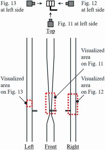
Figure 11. Front view of hydraulic behavior at each gas velocity.

Figure 12. Side view of hydraulic behavior at each superficial gas velocity.

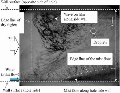
Figure 13. Local snapshot of hydraulic behavior in diffuser part.

Figures 11 and 12 show the overall hydraulic behaviors with increasing superficial gas velocity. In Figures 11 and 12, (a) represents the superficial gas velocity of 82 m/s, (b) 124 m/s, (c) 165 m/s, (d) 210 m/s, (e) 249 m/s, and (f) 290 m/s. In Figure 11, jet breakup can be observed in the throat part. The jet-like wavy band in the throat part and the related droplet generation were observed for gas velocities of 82–165 m/s. With increasing superficial gas velocity, the jet seemed to shorten, and the droplet size decreased. From 201 to 290 m/s, the jet was almost invisible, and the suctioned liquid formed the film flow. Vortexes, a reversed flow, and droplet generation from the liquid film on the diffuser part can be observed from 28 mm to 48 mm in Figures 11 and 12. The number of droplets was large, droplet size was small, and the droplets formed a dispersed flow similar to a mist flow. With increasing superficial gas velocity, the mist-like flow disappeared, and the image obtained in this area cleared up. In addition, the droplet-generation position moved downstream. At superficial gas velocities higher than 330 m/s, self-priming suspension occurred, and a two-phase flow was not observed.

3.5. Droplet generation behavior in throat and diffuser part in Venturi scrubber

The droplet-generation behavior in the diffuser part was visualized using the same method as that used for droplet visualization. Figure 13 shows a snapshot of the side view of the detailed hydraulic behavior of droplet generation at the superficial gas velocity of 317 m/s. This superficial gas velocity condition was selected to observe the hydraulic behavior, including droplet generation. In Figure 13, the position of the visualized area is 10–20 mm downstream of the hole. The gas and the liquid film flow from the left to the right in the figure. The film flow was formed from the jet at the hole. In the left part of the figure, upstream of the observed area, droplets and waves on the liquid film were not observed, and a very clear image was obtained. We called this clear image region ‘dry region.’ In the dry region, a very thin liquid film was present, very few small droplets were generated, and waves could not be observed. The liquid film reached the droplet-generation position shown in Figures 11 and 12, and the liquid film spread to the sidewall. A part of the spread liquid film flowed downstream, but the other part stagnated and waved. In our observations, the droplets were generated from the top of the rippling water periodically. From the liquid film on the hole sidewall, a mist flow with many small droplets was generated locally and flowed downstream. The edge of the mist flow could be observed clearly. The mist flow appeared as a three-dimensional parabola in our visual confirmation.

3.6. Effect of droplet generation by jet breakup in throat part on SMD

Based on the results of the visualization experiment, the droplets were considered to be generated by jet breakup in the throat part of the Venturi scrubber in the superficial gas velocity range of 82–250 m/s. This droplet-generation mechanism is wave formation and growth or jet distortion with steady liquid from the wave edge, as mentioned in [18]. In the experiment conducted to derive the Nukiyama–Tanasawa equation [8–11], sprays were used, and wave formation and growth or jet distortion are known to be components of the atomization mechanism of a spray [19]. Therefore, the Nukiyama–Tanasawa equation could reproduce the droplet diameter of the Venturi scrubber in the superficial gas velocity range of 82–250 m/s because jet breakup at the throat was the dominant mechanism of droplet generation in the Venturi scrubber, and the droplet generation mechanisms was same as those in the Nukiyama–Tanasawa experiment. At superficial gas velocities exceeding 250 m/s, a different droplet generation mechanism was observed in the visualization experiment described in Section 3.5.

The Nukiyama–Tanasawa equation could not obtain a good fit for velocities exceeding 250 m/s because droplet generation from the film in the diffuser part, which was unique to the Venturi scrubber, became dominant and affected SMD. The results obtained using the critical Weber number could not be fit to the experimental results because the droplet-generation mechanism associated with the critical Waver number was not the same as that associated with the Venturi scrubber.

4. Conclusion

To obtain data on the diameters of high-speed droplets in a Venturi scrubber used for filtered venting, a method to measure the droplets generated in the Venturi scrubber under high gas velocities was developed. Droplet diameters in the Venturi scrubber were measured, and by using the measured data, a few equations for evaluating droplet diameter were validated. The reasons why the equations can or cannot evaluate droplet diameter of the Venturi scrubber was considered based on the observed hydraulic behaviors and droplet diameters in the Venturi scrubber. As a result, we arrived at the following conclusions.

• A method to measure the diameters of high-velocity droplets with high-speed video camera, a microscope characterized by a long working distance and a short-pulse laser was developed. By using this method, microscopic droplets moving with a velocity of approximately 60 m/s were visualized.

• Droplet diameter distribution and SMD at higher velocities were determined by visualization and image processing. In addition, it was found that the gamma function can be used to represent the distribution at higher velocities. These findings will be useful to validate several equations used to evaluate droplet diameter.

• The Nukiyama–Tanasawa equation can be used to evaluate SMD in the superficial gas velocity range of 82–250 m/s, but not at 292 m/s. The underlying reason is that in the range of 82–250 m/s, droplets were generated by wave formation and growth in each experiment. At the gas velocity of 292 m/s, the effect of the mist generated in the diffuser part, which seems to be a hydraulic behavior unique to the Venturi scrubber, becomes dominant and the Nukiyama–Tanasawa equation cannot be used to evaluate this mechanism.

Nomenclature

A	=	cross-sectional area [m2]
Cin	=	mass concentration of fission products at inlet [kg/m3]
Cout	=	mass concentration of fission products at outlet [kg/m3]
Dd	=	droplet diameter [m]
Ddi	=	droplet diameter in section i [m]
ΔDdi	=	measurement range of droplet number in section i [m]
DdIP	=	droplet diameter measured by image processing [m]
DdVM	=	droplet diameter measured by visual measurement [m]
Dd10	=	arithmetic mean diameter of droplets [m]
Dd32	=	Sauter mean diameter (SMD) of droplets [m]
Dp	=	particle diameter [m]
EAerosol particles	=	removal efficiency for aerosol particles [-]
EGaseous iodine	=	removal efficiency for gaseous iodine
jG	=	superficial gas velocity [m/s]
jL	=	superficial liquid velocity [m/s]
kG	=	gas-side mass transfer coefficient [m]
$\mathrm{\Delta }l$	=	pixel size [m]
m	=	function of σ0 [-]
$\dot{m}$	=	mass flow rate [kg/s]
N	=	total number of droplets [-]
Δni	=	number of droplets in section i [-]
QG	=	volumetric flow rate of gas [m3/s]
QL	=	volumetric flow rate of liquid in terms of total droplets [m3/s]
r	=	droplet radius [m]
ud	=	droplet velocity [m/s]
uG	=	gas velocity [m/s]
up	=	particle velocity [m/s]
Vd	=	droplet volume [m3]
$t$	=	time [s]
$\mathrm{\Delta }{t}_{ex}$	=	exposure time [s]
Wec	=	critical Weber number [-]
δDd	=	error in droplet diameter [m]
Γ(m)	=	gamma function as a function of m [-]
η	=	impaction efficiency [-]
λ	=	function of m, λ= m
μG	=	gas viscosity coefficient [Pa∙s]
${\rho }_{\mathrm{G}}$	=	gas density [kg/m3]
${\rho }_{\mathrm{p}}$	=	particle density [kg/m3]
${\rho }_{\mathrm{\infty }}$	=	atmospheric gas density [kg/m3]
σ	=	surface tension [N/m]
σ0	=	standard deviation of gamma distribution [-]
ψ	=	inertial coefficient [-]

Acknowledgment

This work was supported by the Japan Atomic Energy Agency.

References

- Lindau L. FILTRA-MVSS_a system for reacter accident mitigation. J Aerosol Sci, 1988; 19(7): 1389–1392,
- Luandilok W, Epstein M, Berger WE Development of the venturi scrubber model for the FILTRA-MVSS system. Proceeding NURETH-13; 2009 Sep 27-Oct 2; Kanazawa (Japan): N13P1255. [CD-ROM].
- Ali M, Yan C, Sun Z, et al. Dust particle removal efficiency of a venturi scrubber. Ann Nucl Energy. 2013;54:178–183.
- Jacquemain D, Guentay S, Basu S, et al. 2014. State report on filtered containment venting. OECD NEA. (NEA/CSNI/R(2014)7).
- Mayinger F, Lehner M. Operating results and aerosol deposition of a venturi scrubber in self-priming operation. Chem Eng Process. 1995;34:283–288.
- Allelein HJ, Auvinen A, Ball J, et al. 2009. State-of-the-art report on nuclear aerosols. OECD NEA. (NEA/CSNI/R(2009)5).
- Ali M, Changoi Y, Zhonging S, et al. Iodine removal efficiency in non-submerged and submerged self-priming venturi scrubber. Nucl Eng Tech. 2013;45(2):203–210.
- Nukiyama S, Tanasawa Y. An experiment on the atomization of liquid by means of an air stream (I). Trans Soc Mech Eng. 1938;4(14):86–93.
- Nukiyama S, Tanasawa Y. An experiment on the atomization of liquid by means of an air stream (II). Trans Soc Mech Eng. 1938;4(15):138–143.
- Nukiyama S, Tanasawa Y. An experiment on the atomization of liquid by means of an air stream (III). Trans Soc Mech Eng. 1939;5(18):63–67.
- Nukiyama S, Tanasawa Y. An experiment on the atomization of liquid by means of an air stream (IV). Trans Soc Mech Eng. 1939;5(18):68–75.
- Guerra VG, Goncalves JAS, Coury JR. Experimental verification of the effect of liquid deposition on droplet size measured in a rectangular venturi scrubber. Chem Eng Proc. 2011;50:1137–1142.
- Horiguchi N, Yoshida H, Kanagawa T, et al. Relationship between flow pattern and pressure distribution in venturi scrubber. Proceeding ICONE22; 2014 Jul 7–11; Prague (Czech Republic): ICONE22-30117 [CD-ROM].
- Horiguchi N, Yoshida H, Kaneko A, et al. Relationship between self-priming and hydraulic behavior in venturi scrubber. Mech Eng J. 2014;1(4):1–11.
- Horiguchi N, Yoshida H, Abe Y. Numerical simulation of two phase flow behavior in venturi scrubber by interface tracking method. Nucl Eng Des. 2016;310:580–586.
- Kolev NI. Multiphase flow dynamics 2. Germany: Springer; 2005. Chap. 8, Acceleration induced droplet and bubble fragmentation; p. 189.
- Horiguchi N, Yoshida H, Kaneko A, et al. Numerical simulation of self-priming phenomena in venturi scrubber by two-phase flow simulation code TPFIT. Proc. ICONE23; 2015 May 17–21; Chiba (Japan): ICONE23-1803 [CD-ROM].
- Goncalves JAS, Costa MAM, Henrique PR, et al. Atomization of liquids in a pease-Anthony Venturi scrubber Part I. Jet dynamics. J Hazardous Mate. 2003;B97:267–279.
- JSME. Atomization technology. Japan; 2008. Chap. 1, Atomization mechanism [in Japanese].