Novel fluctuation reduction procedure for nuclear reactivity calculations based on the discrete fourier transform method

ABSTRACT

A new method for calculating nuclear reactivity based on the Discrete Fourier Transform (DFT) – with two filters: a first-order delay low-pass filter and a Savitzky-Golay filter – is presented. The reactivity is calculated from an integrodifferential equation known as the inverse point kinetic equation, which contains the history of neutron population density. The new method can be understood as a convolution between the neutron population density signal and the response to the characteristic impulse of a linear system. The proposed method is based on the discrete Fourier transform (DFT) that performs a circular convolution. The fast Fourier transform algorithm (FFT) with the zero-padding technique is implemented to reduce the computational cost.

KEYWORDS:

• Reactivity
• nuclear power plant
• nuclear reactor
• numerical simulation

1. Introduction

The development of a country is linked to its production of energy. There are different sources to obtain it, one of them is nuclear energy by means of nuclear fission. That is, the neutron bombardment of a radioactive target either of Uranium or Thorium which releases 200 MeV of energy and from zero to several neutrons which in turn collide with more of these atoms to produce even more neutrons. This process creates a chain reaction that must be controlled by keeping the total neutron population constant. A nuclear reactor is designed and built to control the said reaction, its capacity depends on the energy demanded. The reactor is the most important and the most expensive element of a nuclear plant.

In order to safely operate a nuclear plant, the nuclear reactivity must be known with high precision, this is an essential parameter in the reactor core, which comprises the nuclear fuel, cooling channels and control rods which are inserted into the core for controlling the nuclear reactions. The calculation of reactivity is carried out by using the inverse method of point kinetics, which consists in modeling the temporal behavior of the neutron flux. This method is represented by an integrodifferential equation.

There are several methods in the literature for calculating nuclear reactivity based on the discretization of the integral term in the inverse equation of point kinetics, known as the neutron population density history [1–5]. Recently, several methods for calculating nuclear reactivity based on the Laplace Transform [6], the finite differences method [7] and the three and five-point Lagrange method [8] have been proposed. In a later publication, the discrete version of the Laplace transform was used to calculate the reactivity using the Savitzky-Golay filter to reduce fluctuations [9]. In a more recent article, reactivity is calculated using the Adams-Bashforth-Moulton method and the Savitzky-Golay filter to reduce fluctuations [10].

The previously mentioned works exhibit some drawbacks that could be improved upon, for instance, in the case of the use of the Laplace transform [6,9] – which uses the history of neutron population density – the convolution is slow and has a computational cost of N², where N is the number of samples. A disadvantage of methods that do not use the history of neutron density population [1–5,7,10] is that they can propagate the errors due to noise, since these are recursive methods that only filter the signal once, hence, when calculating a new value of reactivity, the signal cannot be filtered again.

The motivation for the present work is based on a new formulation for the calculation of nuclear reactivity using the Fast Fourier Transform technique which has a computational cost of $\left(\frac{N}{2}\right)Lo{g}_{2}N$. This computational cost is much smaller compared to that of the Laplace transform [6,9]. This method allows the filtering of the noise in the neutron population density signal several times if necessary, since it is a non-recursive method.

2. Theoretical considerations

It is possible to deduce the neutron transport equation to solve any problem in which neutrons are present, the difficulty is, mainly, that its solution would be hard to obtain even using computers since it is an equation that depends on seven variables. Under certain assumptions, it is possible to arrive at the equations of point kinetics [11],

(1) $\frac{dP(t)}{dt}=\left[\frac{\rho (t)-\beta }{\mathrm{\Lambda }}\right]P(t)+\sum _{i=1}^6{\lambda }_i{C}_i(t)$(1)

(2) $\frac{d{C}_i(t)}{dt}=\frac{{\beta }_i}{\mathrm{\Lambda }}P(t)-{\lambda }_i{C}_i(t),i=1,2,\dots ,6$(2)

With initial conditions

(3) $P(t=0)=P_0$(3)

(4) $C_i(t=0)=\frac{{\beta }_i}{\mathrm{\Lambda }{\lambda }_i}{P}_0,$(4)

where P(t) is the neutron population density, C_i(t) is the concentration of the i-th group of delayed neutrons, ρ(t) is the nuclear reactivity, Λ is the generation time of the instantaneous neutrons, β_i is the effective fraction of the i-th group of delayed neutrons, β is the total fraction of delayed neutrons$\left(\beta =\sum _i\beta {\hspace{0.17em}}_i\right)$, λ_i is the decay constant of the i-th group of delayed neutron precursors.

The equations of point kinetics form a system of strongly coupled nonlinear differential equations which describe the temporal evolution of the distribution of neutrons and the concentration of delayed neutron precursors in the core of a nuclear reactor. The solution of this system depends on the form of the reactivity. Two solutions are known, one for the case of constant reactivity, whose solution is a 7^th – order polynomial [11]. A second case is given for a linear variation of the reactivity with an approximate analytical solution [12].

Solving the system provided by Equations (1(1) $\frac{dP(t)}{dt}=\left[\frac{\rho (t)-\beta }{\mathrm{\Lambda }}\right]P(t)+\sum _{i=1}^6{\lambda }_i{C}_i(t)$(1) –4(4) $C_i(t=0)=\frac{{\beta }_i}{\mathrm{\Lambda }{\lambda }_i}{P}_0,$(4) ), the inverse equation of point kinetics can be obtained [11],

(5) $\rho (t)=\beta +\frac{\mathrm{\Lambda }}{P(t)}\frac{dP(t)}{dt}-\frac{1}{P(t)}\sum _{i=1}^6{\lambda }_i{\beta }_i\left[\frac{⟨P_0⟩}{{\lambda }_i}{e}^{-{\lambda }_{i}t}+\underset{0}{\overset{t}{\int }}{e}^{-{\lambda }_i(t-t^{\prime })}P(t^{\prime })d{t}^{\prime }\right],$(5)

where $⟨P_0⟩$ is the initial condition defined as the average of measurements made for the density of the neutron population, which marks the starting point in the simulations (t = 0). Equation (5)(5) $\rho (t)=\beta +\frac{\mathrm{\Lambda }}{P(t)}\frac{dP(t)}{dt}-\frac{1}{P(t)}\sum _{i=1}^6{\lambda }_i{\beta }_i\left[\frac{⟨P_0⟩}{{\lambda }_i}{e}^{-{\lambda }_{i}t}+\underset{0}{\overset{t}{\int }}{e}^{-{\lambda }_i(t-t^{\prime })}P(t^{\prime })d{t}^{\prime }\right],$(5) is the basis for constructing digital reactivity meters, it is an equation that allows decisions to be made for the control and safe operation of a nuclear reactor, such as moving the control rods, passing water with boron or the coolant.

The integral term in Equation (5)(5) $\rho (t)=\beta +\frac{\mathrm{\Lambda }}{P(t)}\frac{dP(t)}{dt}-\frac{1}{P(t)}\sum _{i=1}^6{\lambda }_i{\beta }_i\left[\frac{⟨P_0⟩}{{\lambda }_i}{e}^{-{\lambda }_{i}t}+\underset{0}{\overset{t}{\int }}{e}^{-{\lambda }_i(t-t^{\prime })}P(t^{\prime })d{t}^{\prime }\right],$(5) is known as the history of the neutron population density since for each time step t, it is necessary to know all the values of the power up to that moment in time. This integral term can be written as

(6) $\underset{0}{\overset{t}{\int }}{e}^{-{\lambda }_i(t-t^{\prime })}P(t^{\prime })d{t}^{\mathrm{\prime }}=\underset{0}{\overset{t}{\int }}{h}_i(t-t^{\prime })P(t^{\prime })d{t}^{\prime }=y_i(t),$(6)

where $h_i(t)=e^{-{\lambda }_{i}t}$.

This integral can be solved by approximating the area under the curve through the zero-order numerical summation process [13]. Assuming that N samples of P[n] and h_i[n] are used, it can be approximated by

(7) $y_i(t)\approx y[n]=T\sum _{m=0}^{N-1}{h}_i[n-m]P[m],$(7)

where $T$ is the time step.

On the other hand, the discrete Fourier transform of the periodic digital signals P[n] and h[n] are defined as [14],

(8) $DFT\left\{P[n]\right\}=P[k]=\sum _{n=0}^{N-1}P[n]W_N^{kn},\mathrm{f}\mathrm{o}\mathrm{r}0\le k\le N-1$(8)

(9) $DFT\{h[n]\}=H[k]=\sum _{n=0}^{N-1}h[n]W_N^{kn},\mathrm{f}\mathrm{o}\mathrm{r}0\le ?k\le N-1,$(9)

where

(10) $W_N=e^{-j\frac{2\pi }{N}}$(10)

N is the sample size taken in a time period.

The digital signals P[k] and H[k] for the Inverse Discrete Fourier transform (IDFT) are defined by

(11) $P[n]=\frac{1}{N}\sum _{k=0}^{N-1}P[k]W_N^{-kn},for0\le n\le N-1$(11)

(12) $h[n]=\frac{1}{N}\sum _{k=0}^{N-1}H[k]W_N^{-kn},for0\le n\le N-1,$(12)

where k indicates the frequency space and n the time-space of the signals.

The only differences between the DFT and the IDFT are the factor (1/N) and the negative exponent in the IDFT. Since an algorithm for the calculation of the DFT exists, multiplying the DFT by 1/N and reversing the order of the elements produces an algorithm for the IDFT. The efficient algorithm used for the DFT and IDFT is called the fast Fourier transform (FFT).

Next, the relationship of Equation (7)(7) $y_i(t)\approx y[n]=T\sum _{m=0}^{N-1}{h}_i[n-m]P[m],$(7) with the DFT is shown. Let Y[k] be the DFT of the signal y[n], being equal to the product of the Equations (8(8) $DFT\left\{P[n]\right\}=P[k]=\sum _{n=0}^{N-1}P[n]W_N^{kn},\mathrm{f}\mathrm{o}\mathrm{r}0\le k\le N-1$(8) –9(9) $DFT\{h[n]\}=H[k]=\sum _{n=0}^{N-1}h[n]W_N^{kn},\mathrm{f}\mathrm{o}\mathrm{r}0\le ?k\le N-1,$(9) ), then we can write:

(13) $Y[k]=H[k]P[k].$(13)

Applying the inverse transform to Equation (13)(13) $Y[k]=H[k]P[k].$(13) we have

(14) $y[n]=\frac{1}{N}\sum _{k=0}^{N-1}H[k]P[k]W_N^{-kn}$(14)

Replacing Equation (8)(8) $DFT\left\{P[n]\right\}=P[k]=\sum _{n=0}^{N-1}P[n]W_N^{kn},\mathrm{f}\mathrm{o}\mathrm{r}0\le k\le N-1$(8) into Equation (14)(14) $y[n]=\frac{1}{N}\sum _{k=0}^{N-1}H[k]P[k]W_N^{-kn}$(14) we get

(15) $y[n]=\frac{1}{N}\sum _{k=0}^{N-1}H[k]\left(\sum _{l=0}^{N-1}P[l]W_N^{kl}\right)W_N^{-kn}$(15)

Putting together the summations in Equation (15)(15) $y[n]=\frac{1}{N}\sum _{k=0}^{N-1}H[k]\left(\sum _{l=0}^{N-1}P[l]W_N^{kl}\right)W_N^{-kn}$(15) we can write

(16) $y[n]=\frac{1}{N}\sum _{k=0}^{N-1}\sum _{l=0}^{N-1}H[k]P[l]W_N^{(l-n)k}$(16)

we can introduce the (1/N) factor into Equation (16)(16) $y[n]=\frac{1}{N}\sum _{k=0}^{N-1}\sum _{l=0}^{N-1}H[k]P[l]W_N^{(l-n)k}$(16) to get

(17) $y[n]=\sum _{l=0}^{N-1}P[l]\frac{1}{N}\sum _{k=0}^{N-1}H[k]W_N^{-(n-l)k}$(17)

Using Equation (12)(12) $h[n]=\frac{1}{N}\sum _{k=0}^{N-1}H[k]W_N^{-kn},for0\le n\le N-1,$(12) in Equation (17)(17) $y[n]=\sum _{l=0}^{N-1}P[l]\frac{1}{N}\sum _{k=0}^{N-1}H[k]W_N^{-(n-l)k}$(17) we obtain

(18) $y[n]=\sum _{l=0}^{N-1}P[l]h[n-l]$(18)

With an analogous procedure, Equation (9)(9) $DFT\{h[n]\}=H[k]=\sum _{n=0}^{N-1}h[n]W_N^{kn},\mathrm{f}\mathrm{o}\mathrm{r}0\le ?k\le N-1,$(9) can be replaced in Equation (14)(14) $y[n]=\frac{1}{N}\sum _{k=0}^{N-1}H[k]P[k]W_N^{-kn}$(14) to demonstrate the commutative property, that is

(19) $y[n]=\sum _{l=0}^{N-1}P[l]h[n-l]=\sum _{l=0}^{N-1}P[n-l]h[l]$(19)

Equation (18)(18) $y[n]=\sum _{l=0}^{N-1}P[l]h[n-l]$(18) is the same as Equation (7)(7) $y_i(t)\approx y[n]=T\sum _{m=0}^{N-1}{h}_i[n-m]P[m],$(7) , where m and l are dummy variables.

Thus, by taking the inverse of Y[k] in Equation (13)(13) $Y[k]=H[k]P[k].$(13) , we have the convolution property of the DFT for an output signal and y[n] is given by the following relation:

(20) $y[n]=IDFT\left\{DFT\left\{P[n]\right\}DFT\left\{h[n]\right\}\right\}$(20)

We have seen how Equation (7)(7) $y_i(t)\approx y[n]=T\sum _{m=0}^{N-1}{h}_i[n-m]P[m],$(7) is a zero-order numerical sum approximation of Equation (6)(6) $\underset{0}{\overset{t}{\int }}{e}^{-{\lambda }_i(t-t^{\prime })}P(t^{\prime })d{t}^{\mathrm{\prime }}=\underset{0}{\overset{t}{\int }}{h}_i(t-t^{\prime })P(t^{\prime })d{t}^{\prime }=y_i(t),$(6) , which can be interpreted as Equation (19)(19) $y[n]=\sum _{l=0}^{N-1}P[l]h[n-l]=\sum _{l=0}^{N-1}P[n-l]h[l]$(19) from the Fourier transform just by multiplying by the time step T. But there is a difference, Equation (7)(7) $y_i(t)\approx y[n]=T\sum _{m=0}^{N-1}{h}_i[n-m]P[m],$(7) makes a linear convolution, whilst Equation (19)(19) $y[n]=\sum _{l=0}^{N-1}P[l]h[n-l]=\sum _{l=0}^{N-1}P[n-l]h[l]$(19) makes a circular convolution that can become linear if zeros are added. That is known as the zero-padding technique [14].

Equating Equation (7)(7) $y_i(t)\approx y[n]=T\sum _{m=0}^{N-1}{h}_i[n-m]P[m],$(7) to Equation (20)(20) $y[n]=IDFT\left\{DFT\left\{P[n]\right\}DFT\left\{h[n]\right\}\right\}$(20) and replacing it into Equation (5)(5) $\rho (t)=\beta +\frac{\mathrm{\Lambda }}{P(t)}\frac{dP(t)}{dt}-\frac{1}{P(t)}\sum _{i=1}^6{\lambda }_i{\beta }_i\left[\frac{⟨P_0⟩}{{\lambda }_i}{e}^{-{\lambda }_{i}t}+\underset{0}{\overset{t}{\int }}{e}^{-{\lambda }_i(t-t^{\prime })}P(t^{\prime })d{t}^{\prime }\right],$(5) we get:

(21) $\rho (t)=\beta +\frac{\mathrm{\Lambda }}{P(t)}\frac{dP(t)}{dt}-\frac{⟨P_0⟩}{P(t)}\sum _{i=1}^6{\beta }_i{e}^{-{\lambda }_{i}t}-\frac{T}{P(t)}\left[\left(\sum _{i=1}^6{\lambda }_i{\beta }_i{h}_i(t)\right)\otimes P(t)\right]$(21)

where $h_i(t)=e^{-{\lambda }_{i}t}$is the response to the impulse, $T$is the time step and $\otimes$ denotes a circular convolution. Using the distributive property results only in the solution of one single convolution.

Due to the initial condition imposed in the stable state at t = 0, the reactivity is initially null. This condition is not met, however, by Equation (21)(21) $\rho (t)=\beta +\frac{\mathrm{\Lambda }}{P(t)}\frac{dP(t)}{dt}-\frac{⟨P_0⟩}{P(t)}\sum _{i=1}^6{\beta }_i{e}^{-{\lambda }_{i}t}-\frac{T}{P(t)}\left[\left(\sum _{i=1}^6{\lambda }_i{\beta }_i{h}_i(t)\right)\otimes P(t)\right]$(21) and in order to meet this critical order condition in n= 0, y[0] must be null in Equation (7)(7) $y_i(t)\approx y[n]=T\sum _{m=0}^{N-1}{h}_i[n-m]P[m],$(7) , and so the following adjustment is made:

(22) $y^{\ast }[n]=y[n]-\frac{1}{2}\left[h[n]P[0]+h[0]P[n]\right]$(22)

The adjustment given by Equation (22)(22) $y^{\ast }[n]=y[n]-\frac{1}{2}\left[h[n]P[0]+h[0]P[n]\right]$(22) is known as the trapezoidal adjustment and gives better approximations for the calculation of reactivity. The method represented by Equation (21)(21) $\rho (t)=\beta +\frac{\mathrm{\Lambda }}{P(t)}\frac{dP(t)}{dt}-\frac{⟨P_0⟩}{P(t)}\sum _{i=1}^6{\beta }_i{e}^{-{\lambda }_{i}t}-\frac{T}{P(t)}\left[\left(\sum _{i=1}^6{\lambda }_i{\beta }_i{h}_i(t)\right)\otimes P(t)\right]$(21) allows the calculation of reactivity when the measured neutron population density has noise up to a certain standard deviation σ, which can be called resistance to noise. For a standard deviation σ = 0.001 the differential term can cause problems in the calculation of reactivity, and also the term P(t) in the denominator of Equation (21)(21) $\rho (t)=\beta +\frac{\mathrm{\Lambda }}{P(t)}\frac{dP(t)}{dt}-\frac{⟨P_0⟩}{P(t)}\sum _{i=1}^6{\beta }_i{e}^{-{\lambda }_{i}t}-\frac{T}{P(t)}\left[\left(\sum _{i=1}^6{\lambda }_i{\beta }_i{h}_i(t)\right)\otimes P(t)\right]$(21) , which make these equations non-linear. In order to overcome this problem, and reduce the fluctuations in the input signal, two types of digital filters are used. The first filter is applied to the high-frequency noise, for this, we will consider that the fluctuation of neutron population density input signal has a Gaussian distribution and standard deviation σ around the mean value of the measured neutron population density. The second filter is used for low-frequency noise; this is known as a first-order delay low-pass filter. These filters are expressed as [15],

(23) $\overline{P_i}=\frac{1}{N}\sum _{j=1}^N{P}_j$(23)

(24) $P_i=P_{i-1}+\frac{T}{T+\tau }(\overline{P_i}-P_{i-1}),$(24)

where $\overline{P_i}$ is the average measured neutron population density, $P_i$ and $P_{i-1}$denote the filtered neutron population density at steps i and i-1. We considered that $P_i$ and $P_{i-1}$ are not correlated, τ the filter time constant and T the time step for reactivity calculation.

Another filter that is used to reduce fluctuations is known as the Savitzky-Golay – with Gram’s approximation. This filter is expressed as [10],

(25) $\hat{P}(n)=\sum _{j=-M}^M\sum _{i=0}^d\frac{(2i+1){(2M)}^{(i)}}{{(2M+i+1)}^{(i+1)}}{f}_d^M(j)f_d^M(n)P_j,$(25)

where ${f_d}^M(n)$ is a polynomial of degree d which is calculated using the following formula:

(26) $f_d^M(n)=\sum _{i=0}^d\left(\frac{{(-1)}^{i+d}{(i+d)}^{(2i)}{(M+n)}^i}{{(i!)}^2{(2M)}^{(i)}}\right),$(26)

where ${\left(2M\right)}^i=(2M)(2M-1)...(2M-i+1)$ and ${\left(2M\right)}^0=1$ is the generalized factorial function and M is the half width.

Equation (26)(26) $f_d^M(n)=\sum _{i=0}^d\left(\frac{{(-1)}^{i+d}{(i+d)}^{(2i)}{(M+n)}^i}{{(i!)}^2{(2M)}^{(i)}}\right),$(26) is calculated using the recursive formula:

(27) $f_d^M(j)=\frac{2(2i-1)}{i(2M-i+1)}i{g}_{i-1}^M(j)-\frac{(i-1)(2M+i)}{i(2M-i+1)}{g}_{i-2}^M(j),$(27)

where $g_0^M(j)=1$ and $g_{-1}^M(j)=0$.

In this work, in order to reduce the fluctuations in the calculation of reactivity, we used a filtering constant τ = 0.5 s, given by Equation (24)(24) $P_i=P_{i-1}+\frac{T}{T+\tau }(\overline{P_i}-P_{i-1}),$(24) . The mathematical expression of this filter was presented in [1]. Another filter used for reducing fluctuations is given by Equations (25(25) $\hat{P}(n)=\sum _{j=-M}^M\sum _{i=0}^d\frac{(2i+1){(2M)}^{(i)}}{{(2M+i+1)}^{(i+1)}}{f}_d^M(j)f_d^M(n)P_j,$(25) –27(27) $f_d^M(j)=\frac{2(2i-1)}{i(2M-i+1)}i{g}_{i-1}^M(j)-\frac{(i-1)(2M+i)}{i(2M-i+1)}{g}_{i-2}^M(j),$(27) ) known as the Savitzky-Golay filter (see ref [9,10].). The value of M (half width) can take any integer value, in particular, we take M = 112 for all the numerical experiments – as reported in reference [9] – since that corresponds to the minimum difference in the calculation of reactivity.

In order to simulate the noise contained in the neutron population density term, we make:

(28) $P_{k,noise}=P_k+\sigma {\bar{P}}_i{\eta }_N(0,1),$(28)

where $\sigma$ is the standard deviation, ${\eta }_N(0,1)$ denotes a vector of N values with a Gaussian distribution whose mean and standard deviation are zero and unity, respectively. ${\bar{P}}_i$ is the average of the N values of neutron population density, as given by Equation (23)(23) $\overline{P_i}=\frac{1}{N}\sum _{j=1}^N{P}_j$(23) , $P_{k,noise}$ and $P_k$ denote the neutron population density with and without noise at step k, respectively.

Then, we assume that the noise has a Gaussian distribution with a standard deviation around the mean value of the neutron population density, as provided by Equation (28)(28) $P_{k,noise}=P_k+\sigma {\bar{P}}_i{\eta }_N(0,1),$(28) , a pseudo-random number generator from the Matlab randn (‘state’, 2³¹–1) command was used to reproduce some results obtained in this article.

In the following section, the most relevant results carried out by numerical simulation are presented. The reference method is given by the analytical solution of Equation (5)(5) $\rho (t)=\beta +\frac{\mathrm{\Lambda }}{P(t)}\frac{dP(t)}{dt}-\frac{1}{P(t)}\sum _{i=1}^6{\lambda }_i{\beta }_i\left[\frac{⟨P_0⟩}{{\lambda }_i}{e}^{-{\lambda }_{i}t}+\underset{0}{\overset{t}{\int }}{e}^{-{\lambda }_i(t-t^{\prime })}P(t^{\prime })d{t}^{\prime }\right],$(5) , the proposed method using the FFT is given by Equation (21)(21) $\rho (t)=\beta +\frac{\mathrm{\Lambda }}{P(t)}\frac{dP(t)}{dt}-\frac{⟨P_0⟩}{P(t)}\sum _{i=1}^6{\beta }_i{e}^{-{\lambda }_{i}t}-\frac{T}{P(t)}\left[\left(\sum _{i=1}^6{\lambda }_i{\beta }_i{h}_i(t)\right)\otimes P(t)\right]$(21) , the low-pass filter of first-order delay to reduce the fluctuations in the calculation of reactivity is given by Equation (24)(24) $P_i=P_{i-1}+\frac{T}{T+\tau }(\overline{P_i}-P_{i-1}),$(24) and the Savitzky-Golay filter is given by Equations (25(25) $\hat{P}(n)=\sum _{j=-M}^M\sum _{i=0}^d\frac{(2i+1){(2M)}^{(i)}}{{(2M+i+1)}^{(i+1)}}{f}_d^M(j)f_d^M(n)P_j,$(25) –27(27) $f_d^M(j)=\frac{2(2i-1)}{i(2M-i+1)}i{g}_{i-1}^M(j)-\frac{(i-1)(2M+i)}{i(2M-i+1)}{g}_{i-2}^M(j),$(27) ).

3. Results

In the simulation tests carried out, the parameters: ${\lambda }_i$ the decay constant of delayed neutrons and ${\beta }_i$ the delayed neutron fractions were considered. Table 1 shows the typical coefficients of precursors for a generation time of $\mathrm{\Lambda }=2\times 10{}^{-5}s$.

Table 1. Typical precursor coefficients

Group	1	2	3	4	5	6
λi [s^−1]	0.0127	0.0317	0.115	0.311	1.4	3.87
βi	0.000266	0.001491	0.001316	0.002849	0.000896	0.000182
βi/β	0.0380	0.2130	0.1880	0.4070	0.1280	0.0260

In this work, the difference in reactivity is the error calculated as the absolute value: difference of reactivity = numerical experiment – reference method. The numerical experiment is realized using the proposed method – given by Equation (21)(21) $\rho (t)=\beta +\frac{\mathrm{\Lambda }}{P(t)}\frac{dP(t)}{dt}-\frac{⟨P_0⟩}{P(t)}\sum _{i=1}^6{\beta }_i{e}^{-{\lambda }_{i}t}-\frac{T}{P(t)}\left[\left(\sum _{i=1}^6{\lambda }_i{\beta }_i{h}_i(t)\right)\otimes P(t)\right]$(21) – or the one given by Equations (25(25) $\hat{P}(n)=\sum _{j=-M}^M\sum _{i=0}^d\frac{(2i+1){(2M)}^{(i)}}{{(2M+i+1)}^{(i+1)}}{f}_d^M(j)f_d^M(n)P_j,$(25) –27(27) $f_d^M(j)=\frac{2(2i-1)}{i(2M-i+1)}i{g}_{i-1}^M(j)-\frac{(i-1)(2M+i)}{i(2M-i+1)}{g}_{i-2}^M(j),$(27) ) and the reference method is given by Equation (5)(5) $\rho (t)=\beta +\frac{\mathrm{\Lambda }}{P(t)}\frac{dP(t)}{dt}-\frac{1}{P(t)}\sum _{i=1}^6{\lambda }_i{\beta }_i\left[\frac{⟨P_0⟩}{{\lambda }_i}{e}^{-{\lambda }_{i}t}+\underset{0}{\overset{t}{\int }}{e}^{-{\lambda }_i(t-t^{\prime })}P(t^{\prime })d{t}^{\prime }\right],$(5) . The mean error is the mean value of the vector made up by the differences in reactivity.

Below are some results of numerical experiments developed for different forms of neutron population density. It is worth noticing that the higher mode flux is not considered in this work.

The first numerical experiment consists of assuming an exponential function $P(t)=exp(\omega t)$for the neutron population density term, with ω = 0.016957, where ω is the positive root value of equation “Inhour”. These neutron population density forms imply reactivity values ρ of 100 pcm for simulation times of 300 s. Figure 1 shows that the FFT method is applicable and can reproduce the values obtained with the reference method when the noise contained in the measured neutron population density term has a standard deviation of $\sigma =0.01$, obtaining a maximum difference (Max. Diff in Figures) of 5.45 pcm in $t=2.8s$. 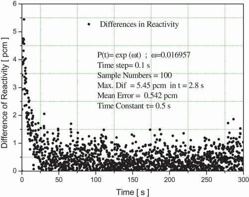This time is very short, as one could wait for a while to observe that the method starts to give better results in the calculation of the reactivity as shown in Figure 2, where the maximum difference after a few seconds is below 2 pcm, which is a lower value compared to that reported in the literature [7] and the mean error in this simulation is approximately 0.542 pcm, which is in good agreement with a recent publication [9].

Figure 1. Variation in nuclear reactivity for a neutron population density factor of $P(t)=exp(0.016957t)$.

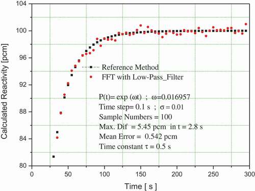
Figure 2. Average error in reactivity for a neutron population density factor of $P(t)=exp(0.016957t)$.

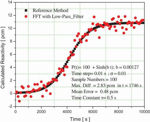
In the second numerical experiment, a neutron population density term of the form $P(t)=100+Sinh(bt)$ with b = 0.00127 and a time step of T= 0.01 s for a total simulation time of 10⁴ s is selected. This neutron population density term produces a variable reactivity of up to 10.84 pcm. Figure 3 shows that for a standard deviation of $\sigma =0.001$, the maximum difference is of 0.29 pcm with a mean error of only 0.05 pcm. Simulating a greater noise with a standard deviation $\sigma =0.01$, which is typical in nuclear reactors, a maximum difference of 2.83 pcm is obtained for an average difference of only 0.48 pcm, as can be observed in Figure 4. These results are consistent with a recent publication [10].

Figure 3. Variation in reactivity for a neutron population density factor of $P(t)=100+Sinh(bt)$ with b = 0.00127 using a standard deviation σ= 0.001.

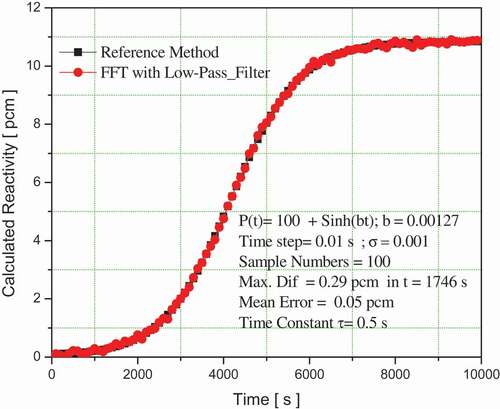
Figure 4. Variation in reactivity for a neutron population density factor of $P(t)=100+Sinh(bt)$ with b = 0.00127 using a standard deviation σ= 0.01.

Tables 2–3 show numerical simulations for several forms of neutron population density, calculation times and different standard deviations. It can be seen that the proposed method using the FFT and the low-pass filter has maximum differences in nuclear reactivity that turn out to be low for standard deviations less than or equal to $\sigma =0.01$for calculation times up to $T=\mathrm{\Delta }t=0.1s$. For this reason, the proposed method could be implemented in a digital reactivity meter.

Table 2. Maximum difference in pcm for several forms of neutron population density with time steps of 0.01 s. Using the first-order delay low-pass filter

Neutron population density	Standard deviation ($\sigma$)	Mean error	Maximum difference (pcm)
$P\left(t\right)=exp\left(\omega t\right);\omega =0.006881$$\mathrm{\Delta }t=0.01s$; (t = 100 s)	0.001	0.31	2.06
	0.01	0.58	2.96
	0.1	4.77	18.47
$P\left(t\right)=exp\left(\omega t\right);\omega =0.01046$$\mathrm{\Delta }t=0.01s$; (t = 100 s)	0.001	0.44	3.12
	0.01	0.67	3.86
	0.1	4.63	17.86
$P\left(t\right)=cosh\left(bt\right);b=0.0123$$\mathrm{\Delta }t=0.01s$; (t = 300 s)	0.001	0.18	0.66
	0.01	0.48	2.22
	0.1	4.43	19.98
$P\left(t\right)=100+\mathbf{S}\mathbf{i}\mathbf{n}\mathbf{h}\left(\mathbf{b}\mathbf{t}\right);b=0.00127$$\mathrm{\Delta }t=0.01s$; (t = 10,000 s)	0.001	0.05	0.29 in t=1746 s
	0.01	0.48	2.83 in t=1746 s
	0.1	4.76	29.46 in t=1746 s

Table 3. Maximum difference in pcm for several forms of neutron population density with time steps of 0.1 s. Using the first-order delay low-pass filter

Neutron population density	Standard deviation ($\sigma$)	Mean error	Maximum difference (pcm)
$P\left(t\right)=exp\left(\omega t\right);\omega =0.006881$$\mathrm{\Delta }t=0.1s$; (t = 100 s)	0.001	0.76	3.02
	0.01	1.36	4.79
	0.1	11.91	51.86
$P\left(t\right)=exp\left(\omega t\right);\omega =0.01046$$\mathrm{\Delta }t=0.1s$; (t = 100 s)	0.001	0.91	4.29
	0.01	1.43	5.70
	0.1	11.58	50.18
$P\left(t\right)=cosh\left(bt\right);b=0.0123$$\mathrm{\Delta }t=0.1s$; (t = 300 s)	0.001	0.59	1.45
	0.01	1.27	5.40
	0.1	11.56	54.83
$P\left(t\right)=100+\mathbf{S}\mathbf{i}\mathbf{n}\mathbf{h}\left(\mathbf{b}\mathbf{t}\right);b=0.00127$$\mathrm{\Delta }t=0.1s$; (t = 10,000 s)	0.001	0.40	1.05
	0.01	1.26	6.94
	0.1	12.18	71.54

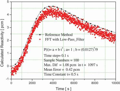
In another experiment, we selected a cubic polynomial form for the neutron population density term $P(t)=a+b{t}^3$ with a = 1 and b = 3.67 * 10^–11 with a standard deviation $\sigma =0.001$ which produces a very low reactivity. The maximum difference when using a calculation time of $T=\mathrm{\Delta }t=0.01s$ turns out to be 0.33 pcm for a time t = 1746 s, with an average error of 0.05 pcm which is negligible, as shown in Figure 5. When the calculation time increases to $T=\mathrm{\Delta }t=0.1s$the maximum difference is 1.08 pcm for a time of t = 1097 s, with a mean error of 0.42 pcm as shown in Figure 6. These results show that the proposed method does not attenuate the reactivity value when compared to the values reported in the literature [7] when the low-pass filter in finite differences was used.

Figure 5. Variation in reactivity for a neutron population density factor of $P(t)=a+b{t}^3$ with a = 1, b= 3.67*10^–11 and time step T= 0.01 s.

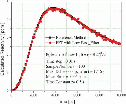
Figure 6. Variation in reactivity for a neutron population density factor of $P(t)=a+b{t}^3$ with a = 1, b= 3.67*10^–11 and time step T = 0.1 s.

Our method has the advantage of using the FFT algorithm, which implies that the noise can be filtered rather than accumulated as it is the case in a recursive process. We considered some forms of the neutron population density with $T=\mathrm{\Delta }t=0.01s$, different standard deviations and several numbers of filtering events, as shown in Table 4. It is observed that when using the proposed method using the FFT and a low pass filter, a slight improvement in the results is obtained for a high standard deviation of $\sigma =0.1$. However, the results improve significantly when the proposed method uses the FFT and the Savitzky-Golay filter to reduce fluctuations in the calculation of reactivity for different forms of the neutron population density and with different standard deviations as shown in Tables 5–6 using $T=\mathrm{\Delta }t=0.01s$ and $T=\mathrm{\Delta }t=0.1s$ respectively. The results can be continually improved upon, that is, with smaller errors if the filters are successively applied, for example, for the neutron population density form $P(t)=100+Sinh(bt)$ with b = 0.00127 and a time step of $T=\mathrm{\Delta }t=0.1s$ for a total simulation time of 10⁴ s, the maximum difference of 7.44 pcm can be achieved using 10 filterings, it can be reduced to 6.26 pcm using 100 filterings and to 4.43 pcm using 1000 filterings.

Table 4. Maximum difference in pcm for several forms of neutron population density with time steps of 0.1 s. Using the first-order delay low-pass filter

Neutron population density	Standard deviation ($\sigma$)	Mean error NoF = 1	Mean error NoF = 5	Mean error NoF = 10	Maximum difference (pcm) NoF = 1	Maximum difference (pcm) NoF = 5	Maximum difference (pcm) NoF = 10
$P\left(t\right)=exp\left(\omega t\right)$$\omega =0.006881$	0.001	0.31	1.51	3.02	2.06	8.26	13.81
	0.01	0.58	1.51	3.00	2.96	7.98	13.60
	0.1	4.77	2.32	3.13	18.47	6.26	11.65
$P\left(t\right)=exp\left(\omega t\right)$$\omega =0.01046$	0.001	0.43	2.14	4.28	3.12	12.47	20.77
	0.01	0.67	2.13	4.26	3.86	12.18	20.56
	0.1	4.63	2.82	4.31	17.86	9.99	18.57
$P\left(t\right)=cosh\left(bt\right)$$b=0.0123$	0.001	0.18	0.84	1.67	0.66	2.49	4.94
	0.01	0.48	0.88	1.68	2.22	2.96	5.13
	0.1	4.43	1.95	2.16	19.98	8.05	8.57

NoF = Number of filterings.

Table 5. Maximum difference in pcm for several forms of neutron population density with time steps of 0.01 s. Using the Savitzky-Golay filter

Neutron population density	Standard deviation ($\sigma$)	Mean error NoF = 1	Mean error NoF = 5	Mean error NoF = 10	Maximum difference (pcm) NoF = 1	Maximum difference (pcm) NoF = 5	Maximum difference (pcm) NoF = 10
$\mathbf{P}\left(\mathbf{t}\right)=exp\left(\omega \mathbf{t}\right)$$\omega =0.006881$	0.001	0.04	0.03	0.03	0.14	0.11	0.10
	0.01	0.40	0.34	0.31	1.45	1.07	0.98
	0.1	4.02	3.39	3.10	14.27	10.80	9.84
$\mathbf{P}\left(\mathbf{t}\right)=exp\left(\omega \mathbf{t}\right)$$\omega =0.01046$	0.001	0.04	0.03	0.03	0.14	0.11	0.10
	0.01	0.39	0.33	0.30	1.42	1.04	0.95
	0.1	3.90	3.29	3.01	13.95	10.51	9.57
$\mathbf{P}\left(\mathbf{t}\right)=exp\left(\omega \mathbf{t}\right)$$\omega =$0.016957	0.001	0.035	0.028	0.026	0.161	0.163	0.155
	0.01	0.348	0.283	0.256	1.526	1.237	1.085
	0.1	3.488	2.840	2.561	15.604	12.595	11.018
$\mathbf{P}\left(\mathbf{t}\right)=cosh\left(\mathbf{b}\mathbf{t}\right)$$\mathbf{b}=0.0123$	0.001	0.04	0.03	0.03	0.16	0.13	0.12
	0.01	0.37	0.30	0.27	1.59	1.29	1.13
	0.1	3.71	3.03	2.73	16.22	13.10	11.47

NoF = Number of filterings.

Table 6. Maximum difference in pcm for several forms of neutron population density with time steps of 0.1 s. Using the Savitzky-Golay filter

Neutron population density	Standard deviation ($\sigma$)	Mean error NoF = 1	Mean error NoF = 5	Mean error NoF = 10	Maximum difference (pcm) NoF = 1	Maximum difference (pcm) NoF = 5	Maximum difference (pcm) NoF = 10
$P\left(t\right)=exp\left(\omega t\right)$$\omega =0.006881$	0.001	0.44	0.45	0.45	2.28	2.27	2.25
	0.01	0.49	0.48	0.51	2.52	2.49	2.33
	0.1	2.87	1.96	1.46	6.22	6.73	6.96
$P\left(t\right)=exp\left(\omega t\right)$$\omega =0.01046$	0.001	0.48	0.48	0.49	3.64	3.61	3.58
	0.01	0.52	0.51	0.54	3.89	3.84	3.66
	0.1	2.75	1.87	1.43	6.44	6.16	6.39
$P\left(t\right)=cosh\left(bt\right)$$b=0.0123$	0.001	0.40	0.40	0.40	0.58	0.59	0.61
	0.01	0.43	0.41	0.42	1.57	1.40	1.35
	0.1	2.43	1.83	1.52	11.98	9.77	8.92
$P\left(t\right)=100+\mathbf{S}\mathbf{i}\mathbf{n}\mathbf{h}\left(\mathbf{b}\mathbf{t}\right)$$b=0.00127$	0.001	0.40	0.40	0.40	0.51	0.48	0.47
	0.01	0.42	0.40	0.40	1.48	1.24	1.09
	0.1	2.44	1.87	1.62	11.42	8.99	7.44

NoF = Number of filterings.

4. Conclusions

A new method to reduce fluctuations in the calculation of nuclear reactivity using the inverse point kinetic equation was presented. Our method is based on a discrete version of the Fourier transform that can perform a circular convolution through the implementation of the fast Fourier transform (FFT). This method resolves the neutron population density history with a zero – order approximation, which is improved with the trapezoidal approximation to meet the criticality condition. In order to reduce fluctuations, a first-order delay low-pass filter and a Savitzky-Golay filter were used, assuming that the measured neutron population density has a Gaussian noise distribution around the average neutron population density with a standard deviation of up to σ = 0.01 and with calculation times up to t = 0.1 s. The best results are obtained using the FFT and a Savitzky-Golay filter with different numbers of filterings of the neutron population density history.

Acknowledgments

The authors thank the research seed of Computational Physics, the research group in Applied Physics FIASUR, and the academic and financial support of the Universidad Surcolombiana.

Disclosure statement

No potential conflict of interest was reported by the authors.

References

- Shimazu Y, Nakano Y, Tahara Y, Okayama T. Development of a compact digital reactivity meter and a reactor physics data processor. Nucl Technol. 1987;77:247–254.
- Ansari SA. Development of on-line reactivity meter for nuclear reactors. IEEE Trans Nucl Sci. 1991;38:946–952.
- Binney SE, Bakir AIM. Design and development of a personal computer based reactivity meter for a nuclear reactor. Nucl Technol. 1989;85:12–21.
- Hoogenboom JE, Van Der Sluijs AR. Neutron source strength determination for on-line reactivity measurements. Ann Nucl Energy. 1988;15:553–559.
- Tamura S. Signal fluctuation and neutron source in inverse kinetics method for reactivity measurement in the sub-critical domain. J Nucl SciTechnol. 2003;40:153–157.
- Suescún DD, Senra AM, Carvalho Da Silva F. Calculation of reactivity using a finite impulse response filter. Ann Nucl Energy. 2008;35:472–477.
- Suescún DD, Senra AM. Finite difference with exponential filtering in the calculation of reactivity. Kerntechnik. 2010;75:210–213.
- Malmir H, Vosoughi N. On-line reactivity calculation using Lagrange method. Ann Nucl Energy. 2013;62:463–467.
- Suescún DD, Bonilla HFL, Figueroa JJH. Savitzky-Golay filter for reactivity calculation. J Nucl Sci Technol. 2016;53:944–950.
- Suescún DD, Rasero CDA, Figueroa JJH. Adams-Bashforth-Moulton method with Savitzky-Golay filter to reduce reactivity fluctuations. Kerntechnik. 2017;82:674–677.
- Duderstadt JJ, Hamilton LJ. Nuclear reactor analysis. New York (NY): Wiley; 1976.
- Palma DAP, Martinez AS, Gonçalves AC. Analytical solution of point kinetics equations for linear reactivity variation during the start-up of a nuclear reactor. Ann Nucl Energy. 2009;36:1469–1471.
- Haykin S, Veen BV. Signal and system. New York (NY): Wiley; 1999.
- Diniz RPS, Da Silva BEA, Netto LS. Digital signal processing: system analysis and design. Cambridge: Cambridge University Press; 2010.
- Kitano A, Itagaki M, Narita M. Memorial-index-based inverse kinetics method for continuous measurement of reactivity and source strength. J Nucl Sci Technol. 2000;37:53–59.