Calculation of the prompt neutron decay constant for the KUCA facility driven by a stationary or pulsed external neutron source

ABSTRACT

In this study, the I-4 configuration of the KUCA facility, as one of the subcritical experimental benchmarks, was examined using computer simulations and experiments. This configuration has all control rods withdrawn. Two different external neutron sources have been analyzed: a pulsed neutron source generated from protons interactions with target materials and a californium neutron source. The two neutron sources have similar spatial effects because the californium neutron source has been located at the position of the proton beam target. Different methods have been applied to calculate the prompt neutron decay constant (alpha) including: the count rate as a function of time fitting, the Rossi, the Feynman, the Cross-Power Spectral Density (CPSD), the Auto-Power Spectral Density (APSD), and the Maρta methods. The input data for these methods consist of the detector timestamps, which can be obtained experimentally using neutron detectors operating in pulse mode or by MCNP fixed-source simulations. The CPSD, the APSD, the count rate fitting, and Maρta methods do not require the detector timestamps since these methods use the average number of neutron counts over some time bins. These averages can be obtained experimentally using detectors operating in the current mode or by MCNP fixed-source simulations.

KEYWORDS:

• Rossi
• Feynman
• spectral density
• decay constant
• KUCA

Introduction

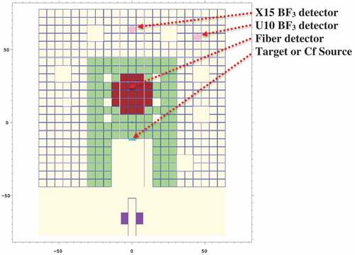
This paper examines the calculations of the prompt neutron decay constant (alpha) of the Kyoto University Critical Assembly KUCA [1,2] using different methods. The main goal of this manuscript is to evaluate how much the alpha values obtained by different methods but the same computational or experimental data differ from one another. The alpha value is obtained from the BF₃ detectors timestamps of the B-10 neutron capture in the detector active zone. These timestamps can be obtained experimentally or by MCNP fixed-source computer simulations [3] and are processed by MATLAB scripts to calculate the alpha value. This study analyzes the I-4 KUCA configuration, which has all control rods withdrawn. The description of this configuration can be found in Refs [4,5]. In this configuration, the facility is driven by an external neutron source, which is generated from protons interactions with a high atomic number material or from the spontaneous fission reactions of californium-252. In the first case, an accelerator produces 100 MeV proton pulses and the proton beam impinges on a tungsten target. The proton pulse duration and period are 100 μs and 50 ms, respectively. The same position is used to place the tungsten target or the californium neutron source. The alpha values have been calculated using the timestamps from three different detectors: two BF₃ detectors located at U10 and X15 positions in the moderator zone and one fiberglass detector located in the fuel zone, as shown in Figure 1. Sections 2 and 3 illustrate the methods to obtain the prompt neutron decay constant for the KUCA facility driven by external neutron sources. Section 4 presents all the obtained alpha results with the different methodologies presented in the previous Sections.

Figure 1. Horizontal section of the KUCA facility; dimensions in cm. Materials legend: light-yellow (air), stainless steel (purple), blue (aluminum), green (polyethylene), cyan (tungsten proton target or Cf source), magenta (indium), pink (BF₃), maroon (fuel).

The MCNP software has been used to provide timestamps with nanosecond precision using the PTRAC and F8 cards, as discussed in Ref [4]. For the noise methods, Rossi, Feynman, and Cross/Auto-Power Spectral Density, the timestamps of the detectors need nanosecond precision for accurate results. For the experimental timestamps, the digital data acquisition system provides timestamps with a precision of 12.5 ns. In addition, the nominal fuel density used in the MCNP simulations has been decreased by 5%, down to 5.44E-2 atoms/b·cm, in accordance with previous studies [4,6]. This decrease has been selected to better match the experimental results (the detector count rate as a function of time), as shown in Ref [4].

Stationary external neutron source

This Section illustrates the various noise methods used to obtain the alpha value when the facility is driven by a californium (stationary) external neutron source located at the tungsten target position. In subcritical systems, unlike in critical systems, the neutron flux does not follow the fundamental mode. Consequently, the position of the detector, relative to the position of the external neutron source, significantly impacts the detector response. In order to set similar detector responses for both the stationary and pulsed external neutron sources, the californium neutron source has been placed at the proton target location. For the stationary external neutron source, the timestamps have been generated by MCNP computer simulations since no experiments were performed with the californium neutron source. Only two methods have been used and they are based on point kinetics and the Rossi and Feynman distributions. These distributions and their calculational procedures are discussed in Refs [4,7]. The prompt neutron decay constant is obtained by fitting the Rossi or Feynman distribution curves using Equations 1(1) $Rossi\left(\tau \right)\cong A+B{e}^{-\alpha \tau }$(1) or 2, respectively [8,9].

(1) $Rossi\left(\tau \right)\cong A+B{e}^{-\alpha \tau }$(1)

(2) $Feynman\left(\tau \right)\equiv \frac{var\left(c\left(\tau \right)\right)}{mean\left(c\left(\tau \right)\right)}-1\cong \frac{B}{{\alpha }^2}\left(1-\frac{1-e^{-\alpha \tau }}{\alpha \tau }\right)$(2)

In Equation 1(1) $Rossi\left(\tau \right)\cong A+B{e}^{-\alpha \tau }$(1) , $\tau$ is the time interval between two neutron capture events, A is a constant set by neutron captures from different fission chains, B is a constant set by neutron captures from the same fission chain, and α is the prompt neutron decay constant. The Rossi distribution peaks when the time interval between two capture events is small since this condition is satisfied for neutrons generated from the same fission chain. Neutrons from the same fission chain contribute only to the second term on the right side of Equation 1(1) $Rossi\left(\tau \right)\cong A+B{e}^{-\alpha \tau }$(1) . In Equation 2(2) $Feynman\left(\tau \right)\equiv \frac{var\left(c\left(\tau \right)\right)}{mean\left(c\left(\tau \right)\right)}-1\cong \frac{B}{{\alpha }^2}\left(1-\frac{1-e^{-\alpha \tau }}{\alpha \tau }\right)$(2) , the Feynman distribution is defined as the ratio between the variance and the mean of the neutron counts c array minus one. The length of the neutron counts array c is defined by the ratio between the experiment time (e.g. 600 seconds) and the arbitrary time interval $\tau$ (e.g. 0.1 ms). Each element of the c array represents the number of neutron counts within the time interval $\tau$. This latter parameter is referred to as the time gate. Consequently, the $\tau$ parameter on the x-axis in the plots of the Rossi and Feynman distributions has a different physical meaning. For the Rossi distribution, the $\tau$ on x-axis represents the time interval between two consecutive neutron captures. For the Feynman distribution, the $\tau$ on x-axis represents the time gate, a time interval of arbitrary size, used for the construction of the c array from the detector timestamps. For each value of the time gate on the x-axis, a different c array is constructed from the detector timestamps.

In the MCNP model, the aluminum sheath of the control rods cells has not been modeled. The fixed-source MCNP calculations of this Section scored 131,049 and 352,534 B-10(n,α) reactions in the BF₃ detector volumes located at positions U10 and X15, respectively, using the PTRAC and F8 cards. The PTRAC card requires analog capture mode, which may have little impact on the Rossi and Feynman distributions [10]. The PTRAC capability of MCNP to obtain the Rossi and Feynman distributions has been also used for the SILENE reactor [11]. The MVP-III Monte Carlo code [12] can calculate the alpha value from the Feynman distribution analysis; however, this code has never been used in this study.

Pulsed external neutron source

Different methods have been used to calculate the prompt neutron decay constant for the KUCA facility driven by a pulsed neutron source. In this case, the timestamps come from either computer simulations or experimental data. The first simplest method for calculating the alpha value is the slope fitting of the detector count rate as a function of time during the decay of prompt neutrons, as discussed and illustrated in Ref. 4. The application of the count rate fitting is straightforward. A single exponential function is fitted in the linear section of the curve when a logarithmic scale is used for the y-axis (the count rate). Additional methods that have been used to calculate the prompt neutron decay constant include fitting the Rossi or Feynman distribution from pulsed neutron sources, using Equations 3(2) $Feynman\left(\tau \right)\equiv \frac{var\left(c\left(\tau \right)\right)}{mean\left(c\left(\tau \right)\right)}-1\cong \frac{B}{{\alpha }^2}\left(1-\frac{1-e^{-\alpha \tau }}{\alpha \tau }\right)$(2) or 4, respectively [13].

(3) $\begin{array}{rl}& Rossi\left(\tau \right)\cong \frac{C_1}{\left({\alpha }_p+{\alpha }_d\right)\left({\alpha }_p-{\alpha }_d\right)}\left(1-\frac{C_2{\lambda }^2}{{\alpha }_p^2}\right)\frac{{\alpha }_p}{2}{e}^{-{\alpha }_p\tau }+\frac{C_1}{\left({\alpha }_p+{\alpha }_d\right)\left({\alpha }_d-{\alpha }_p\right)}\left(1-\frac{C_2{\lambda }^2}{{\alpha }_d^2}\right)\frac{{\alpha }_d}{2}{e}^{-{\alpha }_d\tau }\\ & +C_3\sum _{n=1}^{\mathrm{\infty }}cos{\omega }_n\tau \frac{4\left({\lambda }^2+{\omega }_n^2\right)}{n^2{\pi }^2\left({\alpha }_p^2+{\omega }_n^2\right)\left({\alpha }_d^2+{\omega }_n^2\right)}{\left(sin\frac{{\omega }_{n}W}{2}\right)}^2\end{array}$(3)

(4) $\begin{array}{rl}& Feynman\left(\tau \right)\cong \frac{C_1}{\left({\alpha }_p+{\alpha }_d\right)\left({\alpha }_p-{\alpha }_d\right)}\left(1-\frac{C_2{\lambda }^2}{{\alpha }_p^2}\right)\left(1-\frac{1-e^{-{\alpha }_p\tau }}{{\alpha }_p\tau }\right)+\frac{C_1}{\left({\alpha }_p+{\alpha }_d\right)\left({\alpha }_d-{\alpha }_p\right)}\left(1-\frac{C_2{\lambda }^2}{{\alpha }_d^2}\right)\\ & \left(1-\frac{1-e^{-{\alpha }_d\tau }}{{\alpha }_d\tau }\right)+\frac{C_3}{\tau }\sum _{n=1}^{\mathrm{\infty }}\frac{1}{{\omega }_n^2}{\left(sin\frac{{\omega }_n\tau }{2}\right)}^2\frac{4\left({\lambda }^2+{\omega }_n^2\right)}{n^2{\pi }^2\left({\alpha }_p^2+{\omega }_n^2\right)\left({\alpha }_d^2+{\omega }_n^2\right)}{\left(sin\frac{{\omega }_{n}W}{2}\right)}^2\end{array}$(4)

In Equations 3(2) $Feynman\left(\tau \right)\equiv \frac{var\left(c\left(\tau \right)\right)}{mean\left(c\left(\tau \right)\right)}-1\cong \frac{B}{{\alpha }^2}\left(1-\frac{1-e^{-\alpha \tau }}{\alpha \tau }\right)$(2) and 4(3) $\begin{array}{rl}& Rossi\left(\tau \right)\cong \frac{C_1}{\left({\alpha }_p+{\alpha }_d\right)\left({\alpha }_p-{\alpha }_d\right)}\left(1-\frac{C_2{\lambda }^2}{{\alpha }_p^2}\right)\frac{{\alpha }_p}{2}{e}^{-{\alpha }_p\tau }+\frac{C_1}{\left({\alpha }_p+{\alpha }_d\right)\left({\alpha }_d-{\alpha }_p\right)}\left(1-\frac{C_2{\lambda }^2}{{\alpha }_d^2}\right)\frac{{\alpha }_d}{2}{e}^{-{\alpha }_d\tau }\\ & +C_3\sum _{n=1}^{\mathrm{\infty }}cos{\omega }_n\tau \frac{4\left({\lambda }^2+{\omega }_n^2\right)}{n^2{\pi }^2\left({\alpha }_p^2+{\omega }_n^2\right)\left({\alpha }_d^2+{\omega }_n^2\right)}{\left(sin\frac{{\omega }_{n}W}{2}\right)}^2\end{array}$(3) , the ${\omega }_n$ parameter is defined in Equation 5(5) ${\omega }_n=\frac{2n\pi }{T}$(5) , T is the accelerator pulse period (50 ms), W is the neutron pulse width (100 μs), C_i (with i = 1, 2, or 3) is a constant, λ is the delayed neutrons decay constant, and α_p and α_d are the roots of the inhour equation, which has 2 roots assuming 1 group of delayed neutrons. The prompt neutron decay constant is α_p.

(5) ${\omega }_n=\frac{2n\pi }{T}$(5)

Equations 3(2) $Feynman\left(\tau \right)\equiv \frac{var\left(c\left(\tau \right)\right)}{mean\left(c\left(\tau \right)\right)}-1\cong \frac{B}{{\alpha }^2}\left(1-\frac{1-e^{-\alpha \tau }}{\alpha \tau }\right)$(2) and 4(3) $\begin{array}{rl}& Rossi\left(\tau \right)\cong \frac{C_1}{\left({\alpha }_p+{\alpha }_d\right)\left({\alpha }_p-{\alpha }_d\right)}\left(1-\frac{C_2{\lambda }^2}{{\alpha }_p^2}\right)\frac{{\alpha }_p}{2}{e}^{-{\alpha }_p\tau }+\frac{C_1}{\left({\alpha }_p+{\alpha }_d\right)\left({\alpha }_d-{\alpha }_p\right)}\left(1-\frac{C_2{\lambda }^2}{{\alpha }_d^2}\right)\frac{{\alpha }_d}{2}{e}^{-{\alpha }_d\tau }\\ & +C_3\sum _{n=1}^{\mathrm{\infty }}cos{\omega }_n\tau \frac{4\left({\lambda }^2+{\omega }_n^2\right)}{n^2{\pi }^2\left({\alpha }_p^2+{\omega }_n^2\right)\left({\alpha }_d^2+{\omega }_n^2\right)}{\left(sin\frac{{\omega }_{n}W}{2}\right)}^2\end{array}$(3) have been developed by Kitamura et al. [13]. In Equations 3(2) $Feynman\left(\tau \right)\equiv \frac{var\left(c\left(\tau \right)\right)}{mean\left(c\left(\tau \right)\right)}-1\cong \frac{B}{{\alpha }^2}\left(1-\frac{1-e^{-\alpha \tau }}{\alpha \tau }\right)$(2) and 4(3) $\begin{array}{rl}& Rossi\left(\tau \right)\cong \frac{C_1}{\left({\alpha }_p+{\alpha }_d\right)\left({\alpha }_p-{\alpha }_d\right)}\left(1-\frac{C_2{\lambda }^2}{{\alpha }_p^2}\right)\frac{{\alpha }_p}{2}{e}^{-{\alpha }_p\tau }+\frac{C_1}{\left({\alpha }_p+{\alpha }_d\right)\left({\alpha }_d-{\alpha }_p\right)}\left(1-\frac{C_2{\lambda }^2}{{\alpha }_d^2}\right)\frac{{\alpha }_d}{2}{e}^{-{\alpha }_d\tau }\\ & +C_3\sum _{n=1}^{\mathrm{\infty }}cos{\omega }_n\tau \frac{4\left({\lambda }^2+{\omega }_n^2\right)}{n^2{\pi }^2\left({\alpha }_p^2+{\omega }_n^2\right)\left({\alpha }_d^2+{\omega }_n^2\right)}{\left(sin\frac{{\omega }_{n}W}{2}\right)}^2\end{array}$(3) , the magnitude of the external neutron source affects only the C₃ constant. Consequently, assuming the same facility configuration (including the k_eff value), the sinusoidal oscillations coming from the summation term are amplified by a stronger external neutron source.

In the numerical algorithms used in this study, the upper limit of the summation has been truncated to 1000 because the higher terms give an insignificant contribution to the results. The fitting of the Rossi distribution can be performed using the GNUPLOT software and the scripts listed in the Appendix Section.

Another method to obtain the prompt neutron decay constant is fitting the cross-power spectral density (CPSD) or the auto-power spectral density (APSD). Reference [14] discusses and illustrates these methods and their application to the KUCA experimental data (the detector timestamps) used in this study. The CPSD method uses the timestamps from two detectors and therefore is less sensitive to spatial effects coming from the detector position, relative to other methods. The APSD method uses the timestamps from a single detector.

The last method used to calculate the prompt neutron decay constant is the Maρta method proposed in Refs [15,16]. In this method, it is assumed that the detector count rate P can be written as a combination of some exponential functions as shown in Equation 6(6) $P\left(t\right)\cong b_0+b_1{e}^{-{\alpha }_{1}t}+b_2{e}^{-{\alpha }_{2}t}$(6) and it is proportional to the core power.

(6) $P\left(t\right)\cong b_0+b_1{e}^{-{\alpha }_{1}t}+b_2{e}^{-{\alpha }_{2}t}$(6)

In Equation 6(6) $P\left(t\right)\cong b_0+b_1{e}^{-{\alpha }_{1}t}+b_2{e}^{-{\alpha }_{2}t}$(6) , b_i (with i = 0, 1, 2) and α_j (with j = 1, 2) are the fitting parameters. The detector count rate P is obtained by processing the detector timestamps. Once the fitting parameters of Equation 6(6) $P\left(t\right)\cong b_0+b_1{e}^{-{\alpha }_{1}t}+b_2{e}^{-{\alpha }_{2}t}$(6) are obtained, it is possible to calculate the time derivative of the core power by Equation 7(7) $P^{\prime }\left(t\right)=-{\alpha }_1{b}_1{e}^{-{\alpha }_{1}t}-{\alpha }_2{b}_2{e}^{-{\alpha }_{2}t}$(7) .

(7) $P^{\prime }\left(t\right)=-{\alpha }_1{b}_1{e}^{-{\alpha }_{1}t}-{\alpha }_2{b}_2{e}^{-{\alpha }_{2}t}$(7)

Within the point kinetics analytical framework, it is assumed that Equation 8(8) $C_i=\frac{P\left(T\right){\beta }_{eff}}{{\mathrm{\Lambda }}_{eff}{\lambda }_i}$(8) holds at the end of the pulse period T.

(8) $C_i=\frac{P\left(T\right){\beta }_{eff}}{{\mathrm{\Lambda }}_{eff}{\lambda }_i}$(8)

In Equation 8(8) $C_i=\frac{P\left(T\right){\beta }_{eff}}{{\mathrm{\Lambda }}_{eff}{\lambda }_i}$(8) , C_i is the delayed neutrons precursors concentration for the i group (with i = 1, 2, … 6) of delayed neutrons, ${\beta }_{eff}$ is the delayed neutron fraction, ${\mathrm{\Lambda }}_{eff}$ is the neutron generation time, and λ_i is the precursors decay constant for group i (with i = 1, 2, … 6) of delayed neutrons. In this study, the ${\beta }_{eff}$ and ${\mathrm{\Lambda }}_{eff}$ kinetics parameters were obtained by MCNP criticality simulations, without modeling the external neutron source. The λ_i parameters were obtained from nuclear data libraries. The Maρta method [16] links the core power (Equation 6(6) $P\left(t\right)\cong b_0+b_1{e}^{-{\alpha }_{1}t}+b_2{e}^{-{\alpha }_{2}t}$(6) ), the time derivative of the core power (Equation 7(7) $P^{\prime }\left(t\right)=-{\alpha }_1{b}_1{e}^{-{\alpha }_{1}t}-{\alpha }_2{b}_2{e}^{-{\alpha }_{2}t}$(7) ), and the delayed neutron precursors at the end of the pulse period (Equation 8(8) $C_i=\frac{P\left(T\right){\beta }_{eff}}{{\mathrm{\Lambda }}_{eff}{\lambda }_i}$(8) ) into Equation 9(9) $P^{\prime }\left(t\right)-{\omega }_1\left(t\right)P\left(t\right)-\sum _{i=1}^6\frac{{\lambda }_i{\omega }_1\left(t\right)C_i}{{\omega }_1\left(t\right)+{\lambda }_i}=0$(9) .

(9) $P^{\prime }\left(t\right)-{\omega }_1\left(t\right)P\left(t\right)-\sum _{i=1}^6\frac{{\lambda }_i{\omega }_1\left(t\right)C_i}{{\omega }_1\left(t\right)+{\lambda }_i}=0$(9)

In Equation. 9(8) $C_i=\frac{P\left(T\right){\beta }_{eff}}{{\mathrm{\Lambda }}_{eff}{\lambda }_i}$(8) , it is assumed that the delayed neutron precursors do not change over time and ω₁ is the reactor period. In Equation. 9(8) $C_i=\frac{P\left(T\right){\beta }_{eff}}{{\mathrm{\Lambda }}_{eff}{\lambda }_i}$(8) , the reactor period is a function of time. Equation 9(9) $P^{\prime }\left(t\right)-{\omega }_1\left(t\right)P\left(t\right)-\sum _{i=1}^6\frac{{\lambda }_i{\omega }_1\left(t\right)C_i}{{\omega }_1\left(t\right)+{\lambda }_i}=0$(9) has been solved by MATLAB to obtain the reactor period ω₁ and the core reactivity has been obtained by the in-hour equation, as written in Equation 10(10) $\rho ={\omega }_1\left(T\right){\mathrm{\Lambda }}_{eff}+\sum _{i=1}^6\frac{{\omega }_1\left(T\right){\beta }_i}{{\omega }_1\left(T\right)+{\lambda }_i}$(10) , which has 7 roots, assuming 6 groups of delayed neutrons.

(10) $\rho ={\omega }_1\left(T\right){\mathrm{\Lambda }}_{eff}+\sum _{i=1}^6\frac{{\omega }_1\left(T\right){\beta }_i}{{\omega }_1\left(T\right)+{\lambda }_i}$(10)

Once the reactivity is obtained by Equation 10(10) $\rho ={\omega }_1\left(T\right){\mathrm{\Lambda }}_{eff}+\sum _{i=1}^6\frac{{\omega }_1\left(T\right){\beta }_i}{{\omega }_1\left(T\right)+{\lambda }_i}$(10) , the prompt neutron decay constant (alpha or ω₇) is calculated from Equation 11(11) $\alpha ={\omega }_7\left(T\right)=\frac{\rho -{\beta }_{eff}}{{\mathrm{\Lambda }}_{eff}}$(11) .

(11) $\alpha ={\omega }_7\left(T\right)=\frac{\rho -{\beta }_{eff}}{{\mathrm{\Lambda }}_{eff}}$(11)

The methods based on the Rossi, the Feynman, the CPSD, and the APSD distributions are noise methods [8]. The Rossi and Feynman distribution methods require the use of the detector timestamps. All noise methods assume that once the detector scores one neutron, it will score ν-1 neutrons from the same fission chain and ν neutrons from another (unrelated) fission chain; ν is the number of fission neutrons per fission event. The Rossi and the Feynman distribution methods can be applied to a subcritical assembly driven by either a californium neutron source or a pulsed neutron source. The CPSD and the APSD methods require the use of a pulsed neutron source driving the subcritical assembly, since they are based on frequency domain analyses. The application of the CPSD and APSD methods can be applied using the average neutron count over time intervals. In experiments, the average number of neutron counts as a function of time can be obtained from detectors operating in the current mode or by processing the timestamps of detectors operating in the pulse mode [17]. A discussion about the distinction between the current and the pulse mode detector operation can be found in Ref [7]. The detector pulse mode operation generating timestamps is independent from the pulsed external neutron source parameters set in the proton accelerator. In the experiments of this study, detectors have been always used in pulse mode. In MCNP fixed-source computer simulations, the average number of neutron counts as a function of time can be obtained from the F4 tally results or by processing the timestamps generated by the PTRAC and F8 cards [7]. All the MCNP fixed-source calculations of this study used the PTRAC and F8 card; the F4 card has never been used. The MCNP fixed-source calculations of this Section scored 40,437 and 107,509 B-10(n,α) reactions (by the FM tally multiplier card without modeling the BF₃ gas material) in the BF₃ detector volumes located at positions U10 and X15, respectively. In order to score more neutrons, in the MCNP simulations of this study, the tally volume exceeds the detector volume of the experimental setup. More precisely, the U10 and X15 MCNP tally volumes have 2.5 cm radius and 38 cm height; in the experiment, the U10 and X15 detector volumes have 0.635 and 1.27 cm radius, respectively, and 30 cm height.

The count rate fitting and Maρta methods are not noise methods and do not necessarily require the detector timestamps since they are applied to the count rate as a function of time. Both methods can be only used for a subcritical assembly driven by a particle accelerator operating in pulsed mode.

Results

All computations performed in this study were performed by the Monte Carlo computer program MCNP using the JENDL-4.0 nuclear data library. Different nuclear data libraries were only used for the kinetics parameters summarized in Table 1. These parameters were obtained from MCNP criticality simulations without modeling the external neutron source using ENDF/B-VII, ENDF/B-VIIIβ3, and JENDL-4.0 nuclear data libraries. The delayed neutron fraction and prompt neutron decay constant are insensitive to the used nuclear data library. However, the effective neutron multiplication factors obtained with the ENDF/B nuclear data libraries are 150–300 pcm higher than the value obtained by the JENDL-4.0 nuclear data library.

Table 1. Kinetics parameters obtained from MCNP6 criticality simulations using different nuclear data libraries.

Library	S(α,β)	keff	βeff [pcm]	ρ [μs]
ENDF/B-VIII.β3	ENDF/B-VIII.β3	0.97449 ± 3E-5	809 ± 3	32.57 ± 0.03
ENDF/B-VIII.β3	ENDF/B-VII.1	0.97581 ± 4E-5	812 ± 5	32.65 ± 0.03
ENDF/B-VII.1	ENDF/B-VII.1	0.97549 ± 4E-5	819 ± 5	33.02 ± 0.03
JENDL-4.0	ENDF/B-VII.1	0.97305 ± 4E-5	820 ± 5	33.39 ± 0.04

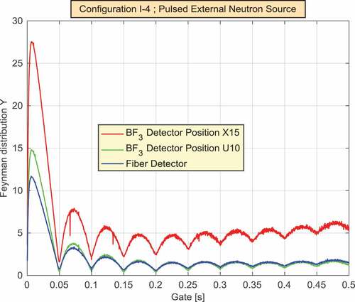
For the KUCA facility driven by a californium external neutron source, all the Rossi and Feynman distributions plots from experimental and computational data are illustrated in Ref. [4], which also shows the fitting of the Rossi, and Feynman distributions to obtain the alpha value. Figure 2 illustrates the Feynman distribution obtained from MCNP simulations for the BF₃ detector located at the U10 position; this plot has not been published in Ref [4]. For the KUCA facility driven by the pulsed neutron source, the neutron count, the Rossi, and the Feynman distributions are illustrated in Figure 3–5, respectively. All these curves have been obtained by MATLAB scripts processing the (pulse mode) detectors timestamps from the experimental data. The experimental data consist of a two-column array and the data in the first column list the timestamps. The Boolean data in the second column can only be 0 or 1; the 0 value indicates the start of an accelerator pulse, whereas the 1 value indicates a B-10(n,α) neutron capture in the detector. The BF₃ detector located at X15 position exhibits the highest count rate since the thermal neutron flux is higher in the reflector zone relative to the fuel zone and this detector is closer to the fuel zone relative to the detector at U10 position. The Rossi distribution peaks when the neutron pulses occur because of the high contribution from neutrons captured from the same fission chain. The Feynman distribution exhibits oscillations that arise from the summation term of Equation 4(4) $\begin{array}{rl}& Feynman\left(\tau \right)\cong \frac{C_1}{\left({\alpha }_p+{\alpha }_d\right)\left({\alpha }_p-{\alpha }_d\right)}\left(1-\frac{C_2{\lambda }^2}{{\alpha }_p^2}\right)\left(1-\frac{1-e^{-{\alpha }_p\tau }}{{\alpha }_p\tau }\right)+\frac{C_1}{\left({\alpha }_p+{\alpha }_d\right)\left({\alpha }_d-{\alpha }_p\right)}\left(1-\frac{C_2{\lambda }^2}{{\alpha }_d^2}\right)\\ & \left(1-\frac{1-e^{-{\alpha }_d\tau }}{{\alpha }_d\tau }\right)+\frac{C_3}{\tau }\sum _{n=1}^{\mathrm{\infty }}\frac{1}{{\omega }_n^2}{\left(sin\frac{{\omega }_n\tau }{2}\right)}^2\frac{4\left({\lambda }^2+{\omega }_n^2\right)}{n^2{\pi }^2\left({\alpha }_p^2+{\omega }_n^2\right)\left({\alpha }_d^2+{\omega }_n^2\right)}{\left(sin\frac{{\omega }_{n}W}{2}\right)}^2\end{array}$(4) . In addition, it dips during the neutron pulses because the pulse neutrons enhance the variance to mean ratio of the c array and lower the Feynman distribution, as can be seen from Equation 2(2) $Feynman\left(\tau \right)\equiv \frac{var\left(c\left(\tau \right)\right)}{mean\left(c\left(\tau \right)\right)}-1\cong \frac{B}{{\alpha }^2}\left(1-\frac{1-e^{-\alpha \tau }}{\alpha \tau }\right)$(2) .

Figure 2. Feynman distribution for the BF₃ detector located at U10 position.

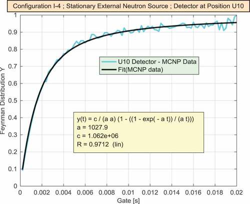
Figure 3. Neutron count as a function of time for three different detectors.

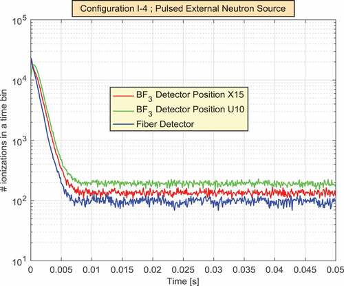
Figure 4. Rossi distribution for three different detectors.

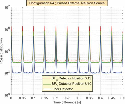
Figure 5. Feynman distribution for three different detectors.

Figure 6 illustrates the Feynman distributions calculated by Argonne National Laboratory and Kyoto University using the same experimental timestamps (but different and independent scripts) for the BF₃ detector located at U10 position; the two distributions overlap. Figures 7 and 8 show the fitting of Figure 6 curves using Equation 4(4) $\begin{array}{rl}& Feynman\left(\tau \right)\cong \frac{C_1}{\left({\alpha }_p+{\alpha }_d\right)\left({\alpha }_p-{\alpha }_d\right)}\left(1-\frac{C_2{\lambda }^2}{{\alpha }_p^2}\right)\left(1-\frac{1-e^{-{\alpha }_p\tau }}{{\alpha }_p\tau }\right)+\frac{C_1}{\left({\alpha }_p+{\alpha }_d\right)\left({\alpha }_d-{\alpha }_p\right)}\left(1-\frac{C_2{\lambda }^2}{{\alpha }_d^2}\right)\\ & \left(1-\frac{1-e^{-{\alpha }_d\tau }}{{\alpha }_d\tau }\right)+\frac{C_3}{\tau }\sum _{n=1}^{\mathrm{\infty }}\frac{1}{{\omega }_n^2}{\left(sin\frac{{\omega }_n\tau }{2}\right)}^2\frac{4\left({\lambda }^2+{\omega }_n^2\right)}{n^2{\pi }^2\left({\alpha }_p^2+{\omega }_n^2\right)\left({\alpha }_d^2+{\omega }_n^2\right)}{\left(sin\frac{{\omega }_{n}W}{2}\right)}^2\end{array}$(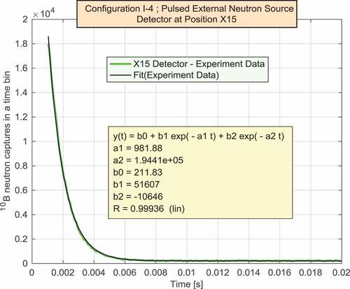4) and GNUPLOT software. The fitting of the Rossi distributions for the BF₃ detectors located at U10 and X15 positions is shown in Figures 9 and 10, respectively. The fitting of the neutron count distributions by Equation 6(6) $P\left(t\right)\cong b_0+b_1{e}^{-{\alpha }_{1}t}+b_2{e}^{-{\alpha }_{2}t}$(6) for the Maρta method and the BF₃ detectors located at U10 and X15 positions is shown in Figures 11 and 12, respectively. All curves shown in Figure 3–12 use experimental timestamps. The fitting of the CPSD and APSD distributions, from the same experimental timestamps of this study, is illustrated in Ref [14].

Figure 6. Feynman distribution for the BF₃ detector located at U10 position. The green and black curves have been produced by Kyoto University and Argonne National Laboratory, respectively, using the same experimental data (detector timestamps).

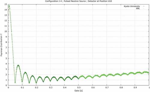
Figure 7. Fitting of the Feynman distribution calculated by Kyoto University (Figure 5) with Equation 4(4) $\begin{array}{rl}& Feynman\left(\tau \right)\cong \frac{C_1}{\left({\alpha }_p+{\alpha }_d\right)\left({\alpha }_p-{\alpha }_d\right)}\left(1-\frac{C_2{\lambda }^2}{{\alpha }_p^2}\right)\left(1-\frac{1-e^{-{\alpha }_p\tau }}{{\alpha }_p\tau }\right)+\frac{C_1}{\left({\alpha }_p+{\alpha }_d\right)\left({\alpha }_d-{\alpha }_p\right)}\left(1-\frac{C_2{\lambda }^2}{{\alpha }_d^2}\right)\\ & \left(1-\frac{1-e^{-{\alpha }_d\tau }}{{\alpha }_d\tau }\right)+\frac{C_3}{\tau }\sum _{n=1}^{\mathrm{\infty }}\frac{1}{{\omega }_n^2}{\left(sin\frac{{\omega }_n\tau }{2}\right)}^2\frac{4\left({\lambda }^2+{\omega }_n^2\right)}{n^2{\pi }^2\left({\alpha }_p^2+{\omega }_n^2\right)\left({\alpha }_d^2+{\omega }_n^2\right)}{\left(sin\frac{{\omega }_{n}W}{2}\right)}^2\end{array}$(4) for the BF₃ detector located at U10 position.

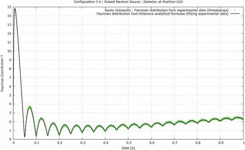
Figure 8. Fitting of the Feynman distribution calculated by Argonne National Laboratory (Figure 5) with Equation 4(4) $\begin{array}{rl}& Feynman\left(\tau \right)\cong \frac{C_1}{\left({\alpha }_p+{\alpha }_d\right)\left({\alpha }_p-{\alpha }_d\right)}\left(1-\frac{C_2{\lambda }^2}{{\alpha }_p^2}\right)\left(1-\frac{1-e^{-{\alpha }_p\tau }}{{\alpha }_p\tau }\right)+\frac{C_1}{\left({\alpha }_p+{\alpha }_d\right)\left({\alpha }_d-{\alpha }_p\right)}\left(1-\frac{C_2{\lambda }^2}{{\alpha }_d^2}\right)\\ & \left(1-\frac{1-e^{-{\alpha }_d\tau }}{{\alpha }_d\tau }\right)+\frac{C_3}{\tau }\sum _{n=1}^{\mathrm{\infty }}\frac{1}{{\omega }_n^2}{\left(sin\frac{{\omega }_n\tau }{2}\right)}^2\frac{4\left({\lambda }^2+{\omega }_n^2\right)}{n^2{\pi }^2\left({\alpha }_p^2+{\omega }_n^2\right)\left({\alpha }_d^2+{\omega }_n^2\right)}{\left(sin\frac{{\omega }_{n}W}{2}\right)}^2\end{array}$(4) for the BF₃ detector located at U10 position.

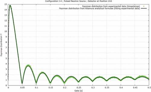
Figure 9. Fitting of the Rossi distribution calculated by Argonne National Laboratory with Equation 3(3) $\begin{array}{rl}& Rossi\left(\tau \right)\cong \frac{C_1}{\left({\alpha }_p+{\alpha }_d\right)\left({\alpha }_p-{\alpha }_d\right)}\left(1-\frac{C_2{\lambda }^2}{{\alpha }_p^2}\right)\frac{{\alpha }_p}{2}{e}^{-{\alpha }_p\tau }+\frac{C_1}{\left({\alpha }_p+{\alpha }_d\right)\left({\alpha }_d-{\alpha }_p\right)}\left(1-\frac{C_2{\lambda }^2}{{\alpha }_d^2}\right)\frac{{\alpha }_d}{2}{e}^{-{\alpha }_d\tau }\\ & +C_3\sum _{n=1}^{\mathrm{\infty }}cos{\omega }_n\tau \frac{4\left({\lambda }^2+{\omega }_n^2\right)}{n^2{\pi }^2\left({\alpha }_p^2+{\omega }_n^2\right)\left({\alpha }_d^2+{\omega }_n^2\right)}{\left(sin\frac{{\omega }_{n}W}{2}\right)}^2\end{array}$(3) for the BF₃ detector at U10 position.

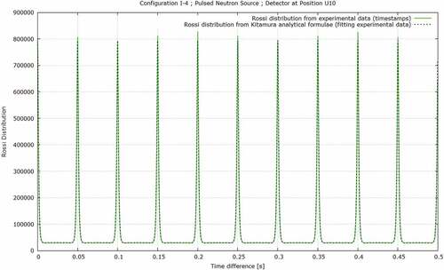
Figure 10. Fitting of the Rossi distribution calculated by Argonne National Laboratory with Equation 3(3) $\begin{array}{rl}& Rossi\left(\tau \right)\cong \frac{C_1}{\left({\alpha }_p+{\alpha }_d\right)\left({\alpha }_p-{\alpha }_d\right)}\left(1-\frac{C_2{\lambda }^2}{{\alpha }_p^2}\right)\frac{{\alpha }_p}{2}{e}^{-{\alpha }_p\tau }+\frac{C_1}{\left({\alpha }_p+{\alpha }_d\right)\left({\alpha }_d-{\alpha }_p\right)}\left(1-\frac{C_2{\lambda }^2}{{\alpha }_d^2}\right)\frac{{\alpha }_d}{2}{e}^{-{\alpha }_d\tau }\\ & +C_3\sum _{n=1}^{\mathrm{\infty }}cos{\omega }_n\tau \frac{4\left({\lambda }^2+{\omega }_n^2\right)}{n^2{\pi }^2\left({\alpha }_p^2+{\omega }_n^2\right)\left({\alpha }_d^2+{\omega }_n^2\right)}{\left(sin\frac{{\omega }_{n}W}{2}\right)}^2\end{array}$(3) for the BF₃ detector at X15 position.

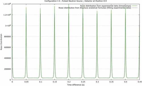
Figure 11. Fitting of the neutron count for the Maρta method and the BF₃ detector located at U10 position.

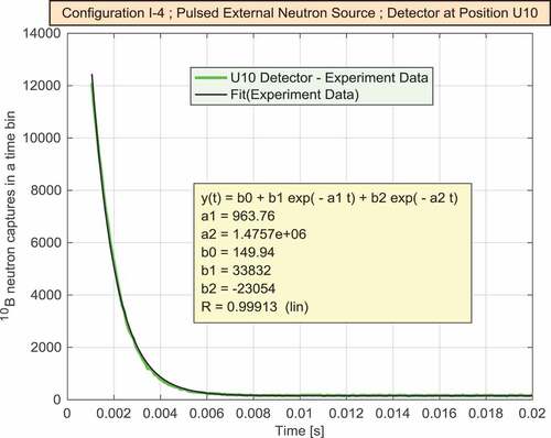
Figure 12. Fitting of the neutron count for the Maρta method and the BF₃ detector located at X15 position.

Table 2 summarizes the values of the prompt neutron decay constant obtained from the different detectors signals using different methods for the I-4 configuration of the KUCA facility. The first column specifies the used neutron source: the fission label refers to the MCNP criticality simulation without external neutron source, the californium label refers to the facility driven by a californium neutron source, the proton label refers to the facility driven by a proton beam interacting with a target material. The second column specifies the source of the timestamps: either experimental values or values obtained from MCNP simulations. The third column defines the used nuclear data library. The fourth Column indicates the used method, all the methods are discussed in Sections 2 and 3 with the exception of the method used for the criticality simulation, which uses Equation 11(11) $\alpha ={\omega }_7\left(T\right)=\frac{\rho -{\beta }_{eff}}{{\mathrm{\Lambda }}_{eff}}$(11) . The fifth column specifies the used detector to obtain the timestamps. The alpha and k_eff values are listed in columns 6 and 7, respectively. The k_eff values have been obtained by using Equation 11(11) $\alpha ={\omega }_7\left(T\right)=\frac{\rho -{\beta }_{eff}}{{\mathrm{\Lambda }}_{eff}}$(11) with the kinetics parameters (β_eff and ρ_eff) from the MCNP criticality simulation. The value in the first row comes from a criticality simulation and therefore it is not subject to corrections related to the detector and the external neutron source location and type. The average alpha values for the detectors at X15 and U10 positions are 977 ± 20 and 979 ± 28 1/s and the average k_eff values from the detectors at X15 and U10 positions are 0.97615 ± 65E-5 and 0.97597 ± 86E-5. The previous statistical errors consist of the standard deviations of the values, which implies all methods are equally reliable. It is beyond the scope of this manuscript to state which method to obtain the alpha value is superior to all others; all methods provide the same alpha value within 3% uncertainty. For this set of experiments, the alpha values obtained by the Maρta method for the BF₃ detectors at positions U10 and X15 are the same.

Table 2. Prompt neutron decay constant obtained by experiments or simulations using different methodologies. The alpha values not discussed in this study are discussed in Refs. [4,14], which also show additional plots on the alpha value calculations.

Neutron Source	Timestamps Source	Data Library	Method	Detector	α [1/s]	keff
Fission	MCNP	JENDL-4.0 ENDF/B-VII.1 S(α,β)	α = (ρ-βeff)/ρ	-	1075 ± 2	0.97305 ± 4E-5
Californium	MCNP	JENDL-4.0 ENDF/B-VII.1 S(α,β)	Rossi Fitting	X15	970 ± 10 [4]	0.97638
Californium	MCNP	JENDL-4.0 ENDF/B-VII.1 S(α,β)	Feynman Fitting	X15	981 ± 6 [4]	0.97603
Proton	MCNP	JENDL-4.0 ENDF/B-VII.1 S(α,β)	Count Rate Fitting	X15	996 ± 4 [4]	0.97556
Proton	Experiment	-	Count Rate Fitting	X15	982 ± 4 [4]	0.97600
Proton	Experiment	-	Maρta	X15	975 ± 2	0.97622
Proton	Experiment	-	Rossi Fitting	X15	938 ± 50	0.97740
Proton	Experiment	-	Feynman Fitting	X15	1000 ± 18	0.97543
Californium	MCNP	JENDL-4.0 ENDF/B-VII.1 S(α,β)	Rossi Fitting	U10	947 ± 30 [4]	0.97712
Californium	MCNP	JENDL-4.0 ENDF/B-VII.1 S(α,β)	Feynman Fitting	U10	1028 ± 15	0.97454
Proton	MCNP	JENDL-4.0 ENDF/B-VII.1 S(α,β)	Count Rate Fitting	U10	987 ± 6 [4]	0.97584
Proton	Experiment	-	Count Rate Fitting	U10	964 ± 4 [4]	0.97657
Proton	Experiment	-	Maρta	U10	975 ± 2	0.97622
Proton	Experiment	-	Rossi Fitting	U10	975 ± 11	0.97622
Proton	Experiment	-	Feynman Fitting	U10	957 ± 19	0.97680
Proton	Experiment	-	CPSD Fitting	U10 & Fiber	958 ± 2 [14]	0.97677
Proton	Experiment	-	APSD Fitting	U10	1019 ± 1 [14]	0.97483

The main burden to obtain the alpha value lies in the experiment or MCNP computation time. The latter can exceed several days, on a cluster of several hundred nodes, because the detector volume to tally the timestamps is small relative to the core volume. Once the timestamps have been acquired or calculated, all Table 2 methods to obtain the alpha value require a few minutes computing time on a desktop. All computations do not require any large RAM memory.

Finally, this study fully integrates with Refs. 4 and 14, which show additional experimental and computational results and plots for the I-4 KUCA configuration. This and previous (Refs. 4 and 14) studies use the same experimental timestamps and MCNP computational model.

Conclusions

This study shows the calculations of the prompt neutron decay constant for the I-4 configuration of the KUCA facility driven by either a stationary (californium) neutron source or a pulsed (proton accelerator) neutron source generated from the proton beam interaction with target materials. The calculation methods for the stationary neutron source configuration include fitting the Rossi and Feynman distributions. The calculation methods for the pulsed neutron source configuration include: fitting the Rossi and Feynman distributions, fitting the peaks of the CPSD and APSD distributions, fitting the count rate as a function of time, and the Maρta method. Noise methods based on the Rossi and Feynman distributions require the detector timestamps, which can be generated from experiments with detectors operating in pulse mode or from MCNP computer simulations with the PTRAC and F8 cards. The CPSD, APSD, fitting the count rate, and Maρta methods do not necessarily require the detector timestamps since they are applied to the average number of neutron counts over time bins. Eventually, the average number of counts over time bins can be constructed from the detectors timestamps. For instance, CPSD, APSD, fitting the count rate and Maρta methods can use the experimental data of detectors operating in current mode or the MCNP simulation results using the F4 tally, without the use of timestamps data. For the BF₃ detectors located at U10 and X15 positions, the average alpha values found in this study are 977 ± 20 and 979 ± 28 1/s and the values obtained by the different methods agree within 3%.

Acknowledgments

The authors acknowledge and thank Prof. Piero Ravetto (Politecnico di Torino) for discussing the Maρta method and Dr. Toshihiro Yamamoto (Kyoto University) for discussing the CPSD and APSD methods.

Disclosure statement

No potential conflict of interest was reported by the authors.

Additional information

Funding

This work is supported by the U.S. Department of Energy, Office of Material Management and Minimization (M3), National Nuclear Security Administration.

APPENDIX

The fitting of the Rossi distribution can be performed using the GNUPLOT software and the following script.

y(x) = c1/((ap+ad)*(ap-ad))*(1-c2*lamda**2/ap**2)*0.5*ap*exp(-ap*x)+

+c1/((ap+ad)*(ad-ap))*(1-c2*lamda**2/ad**2)*0.5*ad*exp(-ad*x)

T0 = 0.05;

w(n) = 2*n*pi/T0;

g(x) = c3*sum[n = 1:1000]cos(w(n)*x)*4*(lamda**2 + w(n)**2)/

/(n**2*pi**2*(ap**2 + w(n)**2)*(ad**2 + w(n)**2))*sin(w(n)*width/2)**2

f(x) = y(x) + g(x) + c4

ap = 971.414; ad = 15.7802; lamda = 0.0753253; width = 0.000992818; c1 = 3.35208e+007; c2 = 121,544; c3 = 5.08641e+013; c4 = 71,188.8;

fit f(x) ‘u10_rossi.data’ using 1:2 via ap,ad,lamda,width,c1,c2,c3,c4

The fitting of the Feynman distribution can be performed using the GNUPLOT software and the following script.

y(x) = c1/((ap+ad)*(ap-ad))*(1-c2*lamda**2/ap**2)*

*(1-(1-exp(-ap*x))/(ap*x))+c1/((ap+ad)*(ad-ap))*

*(1-c2*lamda**2/ad**2)*(1-(1-exp(-ad*x))/(ad*x))

T0 = 0.05;

w(n) = 2*n*pi/T0;

g(x) = (c3/x)*sum[n = 1:1000](1/w(n)**2)*(sin(w(n)*x/2)**2)*4*

*(lamda**2 + w(n)**2)/(n**2*pi**2*(ap**2 + w(n)**2)*

*(ad**2 + w(n)**2))* sin(w(n)*width/2)**2

f(x) = y(x) + g(x)

ap = 957.371; ad = 0.00351491; lamda = 0.280989; width = 0.000168289; c1 = 222,656; c2 = 0.64986; c3 = 6.6487e+013;

fit f(x) ‘u10_feynman.data’ using 1:2 via ap,ad,lamda,width,c1,c2,c3

References

- Pyeon CH, Yagi T, Takahashi Y, et al. Perspectives of research and development of accelerator-driven system in Kyoto University Research Reactor Institute. Prog Nucl Energy. 2015 Jul;82:22–27.
- Pyeon CH, Nakano H, Yamanaka M, et al. Neutron characteristics of solid targets in accelerator-driven system at KYOTO University Critical Assembly. Nucl Tech. 2015 Mar;192(2):181–190.
- Pelowitz DB, Fallgren AJ, McMath GE. MCNP6 user’s manual, code version 6.1.1beta. USA: Los Alamos National Laboratory. LA-CP-14-00745; 2014.
- Talamo A, Gohar Y, Gabrielli F, et al. Advances in the computation of the Sjöstrand, Rossi, and Feynman Distributions. Prog Nucl Energy. 2017 Nov;101:299–311.
- Pyeon CH. Neutronics on solid Pb-Bi in accelerator-driven system with 100 MeV Protons at Kyoto University Critical Assembly. Austria: International Atomic Energy Agency, IAEA; 2014 Nov.
- Pyeon CH, Hervault M, Misawa T, et al. Static and kinetic experiments on accelerator-driven system with 14MeV Neutrons in Kyoto University Critical Assembly. J Nucl Sci Tech. 2008 Jan;45(11):1171–1182.
- Talamo A, Gohar Y. Neutron detector signal processing to calculate the effective neutron multiplication factor of subcritical assemblies. USA: Argonne National Laboratory. ANL-16/14; 2016.
- Pazsit I, Pal L. Neutron fluctuations: A treatise on the physics of branching processes. The Netherlands: Elsevier Science. ISBN-10: 0080450644; 2007.
- Yamanaka M, Pyeon CH, Kim SH, et al. Effective delayed neutron fraction by rossi-α method in accelerator-driven system experiments with 100 MeV Protons at Kyoto University critical assembly. J Nucl Sci Tech. 2017 Jan;54(3):293–300.
- Yamamoto T. Applicability of non-analog Monte Carlo technique to reactor noise simulation. Ann Nucl Energy. 2011 Mar;38(2–3):647–655.
- Humbert P. Simulation and Analysis of List Mode Measurements on SILENE Reactor. J. Comput. Theor. Transport. 2018 Jun;47(4–6):350–363.
- Nagaya Y, Keisuke Okumura K, Sakurai T, et al. MVP/GMVP Version 3: general purpose monte carlo codes for neutron and photon transport calculations based on continuous energy and multigroup methods. JAEA-Data/Code 2016-18. Japan: Japan Atomic Energy Agency; Mar 2017.
- Kitamura Y, Pazsit I, Wright J, et al. Calculation of the pulsed Feynman- and Rossi-alpha Formulae with delayed neutrons. Ann Nucl Energy. 2005 May;32(7):671–692.
- Talamo A, Gohar Y, Yamamoto T, et al. Calculation of the cross and auto power spectral densities for low neutron counting from pulse mode detectors. Ann Nucl Energy. 2019 Sept;131:138–147.
- Dulla S, Hoh SS, Marana G, et al. Analysis of KUCA measurements by the reactivity monitoring MAρTA method. Ann Nucl Energy. 2017 Mar;101:397–407.
- Hoh SS Development of methods for the determination of reactivity from flux measurements in nuclear reactors [Ph.D. Dissertation]. Italy: Politecnico di Torino; 2017.
- Sakon A, Hashimoto K, Sugiyama W, et al. Power spectral analysis for a thermal subcritical reactor system driven by a pulsed 14 MeV neutron source. J Nucl Sci Tech. 2013 Apr;50(5):481–492.