Predictability of a short-term emergency assessment system of the marine environmental radioactivity

ABSTRACT

A Short-Term Emergency Assessment system of the Marine Environmental Radioactivity (STEAMER) was developed at the Japan Atomic Energy Agency (JAEA) to forecast or reanalyze the oceanic dispersion of radionuclides that are released into the ocean around Japan from nuclear facilities during routine operation or in an emergency. STEAMER is currently in daily operation at JAEA to conduct single forecast simulation. The predictability of STEAMER is validated by utilizing oceanographic forecast and reanalysis data in this study. The oceanic dispersion simulations that use oceanographic reanalysis data as input data are assumed to have true solutions. Reanalysis data that has been optimized by data assimilation is the most reliable input for post-analysis. Rigorous oceanic dispersion simulations are conducted for the hypothetical release of Cs-137 from the Fukushima Daiichi Nuclear Power Plant. The predictability of the Cs-137 oceanic dispersion is quantitatively estimated over a forecast period. Moreover, ensemble forecast simulations are also performed applying the Lagged Average Forecast methodology and they successfully improve the predictability of the Cs-137 oceanic dispersion over that obtained using single forecast simulation. The ensemble forecast simulations need to be installed in STEAMER in the future.

KEYWORDS:

• Oceanic dispersion simulation
• cesium 137
• predictability
• STEAMER
• SEA-GEARN
• severe accident
• environment

1. Introduction

Many nuclear facilities, such as nuclear power plants and nuclear fuel reprocessing plants, have been constructed in coastal areas. Therefore, considerable concern has arisen that radionuclides may be routinely released into the ocean from nuclear facilities in operation and accidentally released into the ocean in an emergency. Substantial radionuclides, such as I-131, Cs-134 and Cs-137, were in fact released into the ocean in March 2011 when the tsunami caused by the Great East Japan Earthquake devastated the Fukushima Daiichi Nuclear Power Plant (FNPP1) that was operated by Tokyo Electric Power Company Holdings (TEPCO). In addition, radionuclides could be released into the ocean from other nuclear activities, such as nuclear weapon testing and nuclear waste disposal [1,2]. Given these circumstances, an assessment system that can simulate the oceanic dispersion of radionuclides is required to understand the effect of radionuclides on the marine environment and human activities.

However, there are few assessment systems of oceanic dispersion of radionuclides in the world at present. For example, the French Institute for Radiological Protection and Nuclear Safety (IRSN) has developed emergency response tools for the accidental radiological contamination of French coastal areas [3]. The Japan Atomic Energy Agency (JAEA) has also developed a Short-Term Emergency Assessment system of the Marine Environmental Radioactivity (STEAMER) to forecast or reanalyze the oceanic dispersion of radionuclides in the ocean around Japan [4]. STEAMER is based on an oceanic dispersion model, SEA-GEARN, that was developed at JAEA [5]. STEAMER has been in operation since September 2014 up to the present to evaluate the long-term functioning of this tool. STEAMER receives daily online oceanographic forecast and reanalysis data that is computed by the Japan Meteorological Agency (JMA) and the National Oceanic and Atmospheric Administration (NOAA). Oceanic dispersion simulations are performed daily to forecast the oceanic dispersion of a hypothetical release of Cs-137 from Japanese nuclear facilities using the oceanographic forecast data as input data. The stability of STEAMER has been confirmed thus far over several years of test operations. Recently a downscale methodology was applied to STEAMER to simulate the oceanic condition in the coastal region with a high horizontal resolution [6].

The first purpose of this study is to validate the predictability of STEAMER using oceanographic reanalysis and forecast data. In general, it is difficult to forecast the oceanic dispersion of radionuclides accurately using a single forecast simulation. The second purpose of this study is to improve the predictability of STEAMER using ensemble forecast simulations for future operation. Ensemble forecast simulations are conducted from plural different initial conditions. We can use oceanographic reanalysis and forecast data that we have saved over several years for this validation. The oceanographic forecast is performed using the oceanographic reanalysis data as initial condition. The oceanographic reanalysis data are optimized by data assimilation with abundant observational data to improve accuracy of initial condition. Therefore, the oceanographic reanalysis data are expected to be the most reliable data for post-analysis. Kawamura et al. [7,8] successfully reproduced the Fukushima-induced Cs-137 concentration in the North Pacific and predicted the variation in the oceanic dispersion of Cs-137 using the oceanographic reanalysis data that has been calculated by a similar system to the one used in this study. Therefore, the predictability of STEAMER is validated by conducting oceanic dispersion simulations for the hypothetical release of Cs-137 from FNPP1.

The methodology used in this study is described in Section 2. The simulation results are discussed in Section 3. Lastly, conclusions are presented in Section 4.

2. Methodology

2.1. Oceanographic data

The oceanic dispersion of radionuclides is strongly dependent on ocean currents. STEAMER receives oceanographic data, including ocean currents, temperature, salinity, and sea surface height, that are computed by JMA and NOAA on line daily. This input data are used by STEAMER to forecast the oceanic dispersion of radionuclides. JMA provides the oceanographic 30-day forecast and reanalysis (nowcast) data that are computed using an ocean data assimilation system described below with horizontal resolutions of 1/10° for the western North Pacific around Japan and 1/2° for the North Pacific through the Japan Meteorological Business Support Center. NOAA also provides the oceanographic 8-day forecast and reanalysis (nowcast) data that are computed using the global operational Real-Time Ocean Forecast System (RTOFS-Global) at the National Centers for Environmental Prediction with a horizontal resolution of 1/12° for the global ocean [9].

In this study, the predictability of STEAMER is validated using oceanographic forecast and reanalysis data computed by JMA for the western North Pacific around Japan. The datasets are compiled over a long forecast period (30 days) and have relatively high horizontal resolution (1/10°). The oceanographic reanalysis data are optimized using Multivariate Ocean Variational Estimation (MOVE) [10], which was developed at the Meteorological Research Institute (MRI) of JMA. MRI of JMA used the MRI Community Ocean Model (MRI.COM) [11] to develop an ocean data assimilation system MOVE/MRI.COM. Data assimilation is the synthesis of numerical models and observational data to produce optimal data. Satellite data for the sea surface temperature and height and in situ temperature and salinity data are assimilated in MOVE/MRI.COM using a three-dimensional variational adjoint method (3DVAR) to optimize the initial oceanic condition (nowcast) for numerical forecasting. There are four versions of MOVE/MRI.COM: a global and atmosphere-ocean coupled version (MOVE/MRI.COM-C), a global version (MOVE/MRI.COM-G), a North Pacific version (MOVE/MRI.COM-NP), and a western North Pacific version (MOVE/MRI.COM-WNP). The oceanographic data used in this study for the ocean around Japan is computed by MOVE/MRI.COM-WNP with a horizontal resolution of 1/10° and 54 vertical layers.

The oceanographic reanalysis data that are optimized by data assimilation are often used to analyze past oceanographic phenomena. The oceanographic reanalysis data, as well as the oceanographic forecast data, has been saved from September 2014 up to the present in STEAMER. In this study, oceanographic forecast and reanalysis data are used from the past three years (2015–2017).

2.2. Oceanic dispersion model

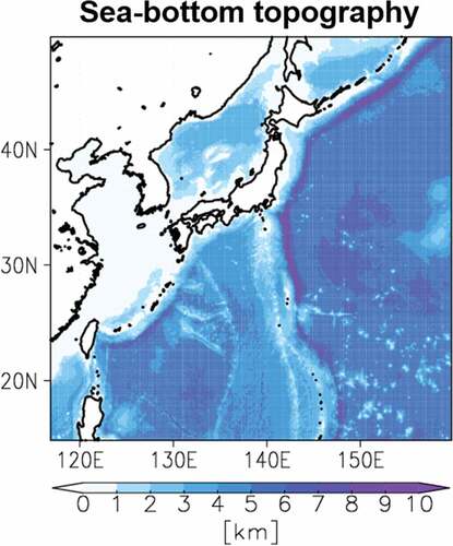
The SEA-GEARN model that is used in this study to simulate the oceanic dispersion of radionuclides is a Lagrangian particle random-walk model [5]. The model domain extends from 14.85°N to 49.75°N in latitude and from 116.85°E to 159.75°E in longitude (Figure 1) for a horizontal resolution of 1/10° and 54 vertical layers. The horizontal and vertical resolutions of SEA-GEARN are same as those of MOVE/MRI.COM-WNP in the western North Pacific around Japan. The time step is set at 360 s. The diffusion process of radionuclides is solved using a random-walk methodology. The horizontal diffusion coefficient is calculated using the Smagorinsky formula [12] and horizontal ocean current data. The vertical diffusion coefficient is set at a constant value of 10⁻⁵ m² s⁻¹. The ocean current data, as computed by MOVE/MRI.COM-WNP, are input with a 1-day interval to the oceanic dispersion simulations. The detailed configuration of SEA-GEARN is summarized in Table 1.

Table 1. SEA-GEARN configuration.

Simulation period	30 days from the first day of every month from 2015 to 2017
Model domain	Western North Pacific
	14.85°N–49.75°N, 116.85°E–159.75°E
Time step	360 s
Horizontal resolution	0.1° for latitude and longitude
Vertical resolution	54 layers
Horizontal diffusion coefficient	Smagorinsky formula
Vertical diffusion coefficient	10^−5 m^2 s^−1
Input oceanographic data	Ocean current data computed by MOVE/MRI.COM-WNP
	1-day interval
Maximum particle number	15,897,600
Radionuclide	Cs-137 (half-life: 30 years)
Release period	30 days (continuous release)
Release point	37.42°N, 141.15°E, sea surface
Release rate	1 Bq h^−1

Figure 1. Sea-bottom topography (km) in the model domain.

This study focuses on Cs-137, which is an important radionuclide for assessing the marine environmental radioactivity in a nuclear severe accident. SEA-GEARN accounts for the interactions among three radionuclide phases in the ocean: a dissolved phase in seawater, an adsorbed phase in large particulate matter, and an adsorbed phase in sea-bottom sediment [5]. In this study, it is assumed that Cs-137 only disperses as a dissolved phase in seawater because the majority of Cs-137 in the ocean remains as this phase. The Cs-137 oceanic dispersion is then calculated by considering the advection and diffusion processes that are caused by ocean currents and radiological decay with a half-life of approximately 30 years.

The oceanic dispersion simulations are conducted over 30 days starting at the first day of each month for 2015, 2016, and 2017. The hypothetical Cs-137 release from FNPP1 is considered to be continuous at a unit release rate of 1 Bq h⁻¹ for 30 days. The release point is set at the sea surface at 37.42°N latitude and 141.15°E longitude. The computation time and statistical error depend on the number of particles. Approximately 1,000,000 particles are assigned for a processor in parallel to save the computation time and suppress the statistical error. As a result, a maximum number of 15,897,600 particles are used to simulate Cs-137 over 30 days by 16 processors in parallel.

The oceanic dispersion simulations that are driven by the oceanographic forecast and reanalysis data are referred to as the ‘forecast simulation’ and the ‘reanalysis simulation,’ respectively, in this study. The results of the reanalysis simulations are assumed to be true solutions and are compared with the results of the forecast simulations to validate the predictability of STEAMER.

2.3. Ensemble forecast simulation

In general, it is difficult to forecast oceanic or atmospheric conditions accurately using a single forecast simulation. This is because in a single forecast simulation, the error including in the initial condition amplifies with time, resulting in forecast error of the oceanic or atmospheric conditions. Recently, ensemble forecast simulations have been extensively employed in oceanography and meteorology to improve forecast precision [13]. An ensemble forecast simulation is often conducted using plural different initial conditions to introduce intentional error. An ensemble forecast simulation can on average improve the predictability of oceanic or atmospheric conditions because of mutual cancelation of the initial errors in the plural forecast simulations.

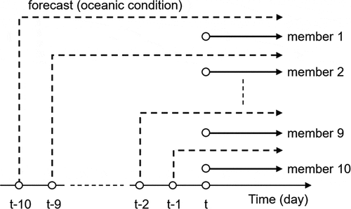
In this study, ensemble forecast simulations are performed to improve the predictability of the Cs-137 oceanic dispersion. We employ the Lagged Average Forecast (LAF) methodology, wherein forecasts are made using plural initial conditions with a constant time interval [14]. In addition to the single forecast simulation, which is referred to as a forecast simulation here, 10 ensemble forecast simulations are performed using 10 oceanographic forecast data (Figure 2). These data are computed from 10 different initial conditions with a time interval of one day during the prior 10 days. In this study, each ensemble forecast simulation is referred to as ‘member 1, 2, 3, 4, 5, 6, 7, 8, 9, and 10.’ For example, the oceanic dispersion simulations are conducted from the first day (t) of the forecast simulations using the oceanographic forecast data that are computed for the prior 10 days (t-10) in member 1. The oceanic dispersion simulations are performed from the same day (t) using the oceanographic forecast data that are computed for the prior 9 days (t-9) in member 2 and so forth. The results of the 10 ensemble members and forecast simulations are averaged to obtain an ensemble mean value for a forecast period of 20 days. The predictability of the ensemble forecast simulations is validated for the period from 2015 to 2017.

Figure 2. Ensemble forecast simulation methodology.

3. Results and discussion

3.1. Predictability of single forecast simulation

The ocean currents in the region off Fukushima Prefecture have a very complex structure because this region includes the Kuroshio Current, the Kuroshio Extension, and the Oyashio Current, all of which vary strongly in space and time [15]. Moreover, many mesoscale eddies with spatial scales of several hundred kilometers are often accompanied with the meander of the Kuroshio Extension. If the radionuclides released from FNPP1 disperse northward in the coastal region, they could be captured by these mesoscale eddies in the offshore region. However, if the radionuclides disperse to the south in the coastal region, they will be entrained into the Kuroshio Extension and carried eastward to the offshore region. Many studies have shown that the radionuclides that were released into the ocean from the FNPP1 accident were largely affected by the Kuroshio Extension and mesoscale eddies [7,8,16–19].

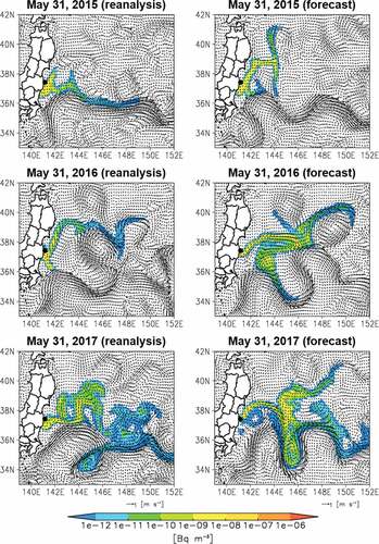
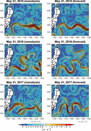
Figure 3 shows the surface Cs-137 concentration 30 days after May 1 in 2015, 2016 and 2017 in the reanalysis and forecast simulations. The reanalysis simulation for the 2015 data shows that the surface Cs-137 is entrained into the Kuroshio Extension and then carried east into the offshore region. However, the forecast simulation for 2015 shows that the surface Cs-137 is mainly dispersed in the northeast direction in the coastal region before being captured by the mesoscale eddies in the offshore region. The remarkable difference between the reanalysis and forecast simulations for 2016 is attributed to the entrainment of the surface Cs-137 into the Kuroshio Extension in the southern offshore region by the westward ocean current in the forecast simulation. Both the reanalysis and forecast simulations for 2017 show that the surface Cs-137 is entrained into the Kuroshio Extension and spreads widely because of the meander of the Kuroshio Extension in the offshore region.

Figure 3. Surface Cs-137 concentration (Bq m⁻³) 30 days after May 1 in 2015 (upper), 2016 (middle), and 2017 (lower): left and right panels show reanalysis and forecast simulations, respectively; vectors show surface horizontal ocean current (m s⁻¹).

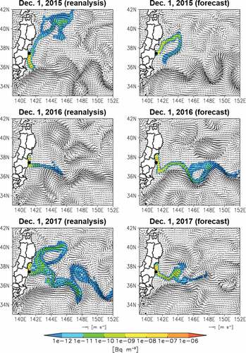
Figure 4 shows the surface Cs-137 concentration 30 days after November 1 in 2015, 2016 and 2017 in the reanalysis and forecast simulations. The reanalysis simulation for 2015 shows that the surface Cs-137 disperses in the north-south direction in the coastal region, is carried in the northeast direction, and then captured by the mesoscale eddies in the offshore region. However, the forecast simulation for 2015 shows the return of the surface Cs-137 in the southwest direction in the offshore region. The reanalysis simulation for 2016 shows that the surface Cs-137 is dispersed straightforward in the east direction in the offshore region. The forecast simulation for 2016 shows similar eastward dispersion of the surface Cs-137, although the transport is much faster than that in the reanalysis simulation. The reanalysis simulation for 2017 shows that the surface Cs-137 is captured by the anticyclonic mesoscale eddy in the northern offshore region and entrained into the Kuroshio Extension in the southern offshore region. The forecast simulation for 2017 shows that the surface Cs-137 disperses in the east and does not spread widely in the offshore region.

Figure 4. Surface Cs-137 concentration (Bq m⁻³) 30 days after November 1; all other notations are the same as those shown in Figure 3.

The differences between the reanalysis and forecast simulations for the 30-day forecast of the Cs-137 concentration can be observed in the surface layer (Figures 3 and 4) as well as the deeper layers. These differences grow with time because of the accumulation of the forecast error in the ocean current. In general, the oceanic condition varies more weakly than the atmospheric condition. However, many factors, such as sea surface wind and heat, can affect the oceanic condition. In particular, it is difficult to forecast the oceanic condition in the Kuroshio Extension because of the high variability and generation of many mesoscale eddies in the region. In addition, the differences between the reanalysis and forecast simulations for the 30-day forecast of the Cs-137 concentration can be also observed in the coastal region near FNPP1 30 days after May 1 in 2017 (Figure 3) and November 1 in 2015 (Figure 4). The oceanic condition in the coastal region is complex, because it is affected by steep topography, coastal wind and so on. A horizontal resolution of 1/10° in this study is insufficient to simulate the oceanic condition in the coastal region accurately. Moreover, the forecast simulation with a horizontal resolution of 1/10° largely depends on the oceanic condition at the release point in the coastal region near FNPP1.

Figure 5 shows the magnitude of the surface horizontal ocean current 30 days after May 1 in 2015, 2016 and 2017 in the reanalysis and forecast simulations. The main axis of the Kuroshio Extension streams from 34°N to 38°N. The reanalysis simulation for 2015 shows that the Kuroshio Extension is relatively stable and streams straightforward to the east. The forecast simulation for 2015 shows similar behavior for the Kuroshio Extension, albeit with a relatively more active meander. Anticyclonic mesoscale eddies are generated off the Tohoku district with a center at 38°N and 144°E in the reanalysis simulation and 40°N and 144°E in the forecast simulation, respectively. The reanalysis simulation for 2016 shows instability and active meandering of the Kuroshio Extension. As a result, many mesoscale eddies are generated along the path of the Kuroshio Extension east of 146°E. However, the forecast simulation for 2016 shows that the axis of the Kuroshio Extension is relatively retained east of 146°E. The difference in the meander of the Kuroshio Extension between the reanalysis and forecast simulations also affects the mesoscale eddies off FNPP1. The mesoscale eddy spreads with a center at 38°N and 143°E in the northeast-southwest direction in the reanalysis simulation, whereas the mesoscale eddy spreads with a center at 38°N and 144°E in the east-west direction in the forecast simulation. This difference in the eddy behavior produces the observed difference in the Cs-137 oceanic dispersion off FNPP1 for May 2016 between the reanalysis and forecast simulations (Figure 3). The forecast simulation for 2017 shows a more intense meander in the Kuroshio Extension relative to that observed in the reanalysis simulation. Another difference between the results of the reanalysis and forecast simulations for 2017 is related to the southward ocean current along the Tohoku district, which is located on the northern part of the main island of Japan. The southward ocean current streams to 37°N off FNPP1 in the reanalysis simulation, whereas it turns to the east, north of 38°N in the forecast simulation. This difference in the behavior of the ocean current causes a corresponding difference in the Cs-137 oceanic dispersion off FNPP1 between the reanalysis and forecast simulations for 2017 (Figure 3).

Figure 5. Surface magnitude of the horizontal ocean current (m s⁻¹) 30 days after May 1 in 2015 (upper), 2016 (middle), and 2017 (lower): left and right panels show reanalysis and forecast simulations, respectively; vectors show surface horizontal ocean current (m s⁻¹).

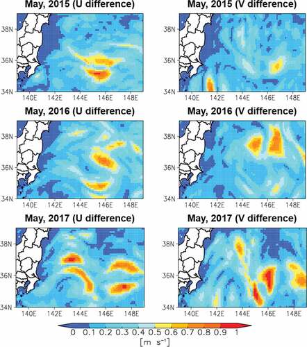
The accumulation of the forecast error in the ocean current over the forecast period is the main reason for the forecast error in the Cs-137 oceanic dispersion. Figure 6 shows the time mean value of the difference between the reanalysis and forecast simulations for the surface zonal and meridional ocean currents for May in 2015, 2016, and 2017. Clear differences between the two simulations can be seen for the surface horizontal ocean current in the Kuroshio Extension region from 34°N to 38°N east of 142°E, which reflects the corresponding differences in the meander of the Kuroshio Extension and the mesoscale eddies. Differences between the results of the two simulations for 2017 are also observable for the surface meridional ocean current in the coastal region near FNPP1, reflecting the difference in the results for the southward ocean current along the Tohoku district.

Figure 6. Time mean value of the difference between the reanalysis and forecast simulations for the surface zonal (left) and meridional (right) ocean currents (m s⁻¹) during the 30 days after May 1 in 2015 (upper), 2016 (middle), and 2017 (lower).

The predictabilities of the oceanic condition and the oceanic dispersion of radionuclides depend on the forecast period. Weather forecasting systems are used to make daily, weekly, and seasonal forecasts in many countries around the world. It is important to validate the predictability of STEAMER using the forecast period that will be regularly used in future operation. The predictability of STEAMER is examined from the point of view of the reproducibility of the significant Cs-137 concentration in the reanalysis simulation. It is not problematic that Cs-137 disperses in some regions in the forecast simulation but not in the reanalysis simulation. In addition, the reproducibility of the Cs-137 concentration within a factor of 10 is considered to be relatively accurate in this study. We defined a predictability indicator (P) as the following equation.

(1) $\mathrm{P}=\frac{N_f}{N_r}\times 100$(1)

N_r: Number of grids (C_r ≥ 10⁻¹² Bq m⁻³)

N_f: Number of grids (C_r × 0.1 ≤ C_f ≤ C_r × 10, C_r ≥ 10⁻¹² Bq m⁻³)

C_r: Cs-137 concentration in the reanalysis simulation

C_f: Cs-137 concentration in the forecast simulation

In Equation (1)(1) $\mathrm{P}=\frac{N_f}{N_r}\times 100$(1) , N_r indicates the number of grids where the Cs-137 concentration (C_r) in the reanalysis simulation is more than 10⁻¹² Bq m⁻³. N_f indicates the number of grids where the Cs-137 concentration (C_f) in the forecast simulation is within a factor of 10 of the Cs-137 concentration in the reanalysis simulation.

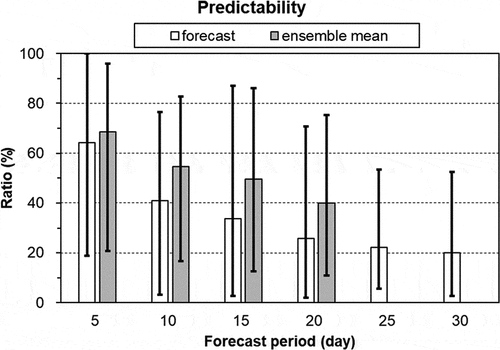
Overall, the predictability of the Cs-137 oceanic dispersion decreases with the forecast period; however, there are variations in the predictability within a forecast period (Figure 7). The predictability indicator attains a maximum value of 100% in February 2016, April 2016, and July 2017 and a minimum value of 19% in November 2017 for the 5-day forecast. The predictability indicator attains a maximum value of 77% in April 2017 and a minimum value of 3% in August 2016 for the 10-day forecast. The predictability indicator attains a maximum value of 87% in October 2017 and a minimum value of 3% in August 2016 for the 15-day forecast. The predictability indicator attains a maximum value of 71% in October 2017 and a minimum value of 2% in October 2015 for the 20-day forecast. The predictability indicator attains a maximum value of 53% in February 2016 and a minimum value of 6% in August 2016 for the 25-day forecast. The predictability indicator attains a maximum value of 53% in February 2016 and a minimum value of 3% in November 2015 for the 30-day forecast. A sufficient number of oceanic dispersion simulations have not been performed in this study; however, the trend in the mean predictability indicator for the period from 2015 to 2017 indicates that the predictability of the Cs-137 oceanic dispersion clearly depends on the forecast period (Figure 8). The mean predictability indicator are calculated to be 64%, 41%, 34%, 26%, 22%, and 20% for the 5-day, 10-day, 15-day, 20-day, 25-day, and 30-day forecasts, respectively.

Figure 7. Predictability indicator (%) for the 5-day, 10-day, 15-day, 20-day, 25-day, and 30-day forecasts.

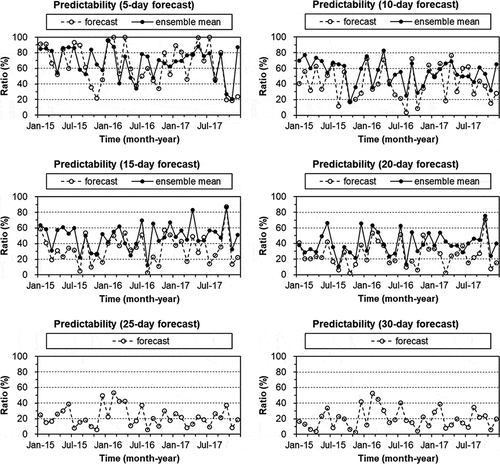
Figure 8. Mean predictability indicator (%) for the period from 2015 to 2017 for the 5-day, 10-day, 15-day, 20-day, 25-day, and 30-day forecasts; bars indicate the range between the minimum and maximum values for the period from 2015 to 2017.

3.2. Predictability of ensemble forecast simulation

The oceanic and atmospheric predictabilities depend on the oceanic and atmospheric conditions, respectively, over the forecast period. If a strong perturbation in the ocean or the atmosphere develops during the forecast period, the oceanic and atmospheric forecast is more difficult to make; conversely, it is easier to make the respective forecasts under smooth conditions. Many research studies have recently been conducted to improve oceanic or atmospheric predictabilities. The ensemble forecast simulation is one of the powerful methodologies that are available to improve oceanic or atmospheric predictabilities. In this study, ensemble forecast simulations employing the LAF methodology [14], as described in subsection 2.3, are used to improve the predictability of the Cs-137 oceanic dispersion.

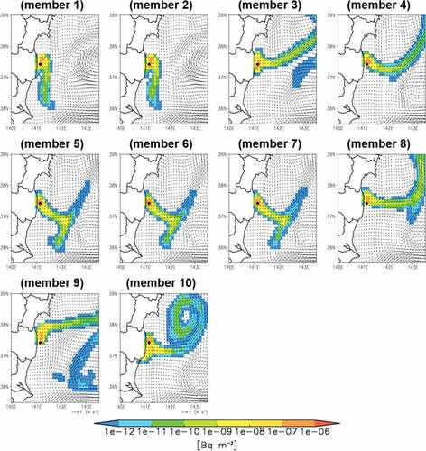
A minimum value (2%) of the predictability indicator is found for the 20-day forecast for October 2015 from the oceanic dispersion simulation (Figure 7). In this case, the reanalysis simulation shows southward Cs-137 oceanic dispersion from FNPP1 along the coast, whereas the forecast simulation shows eastward Cs-137 oceanic dispersion from FNPP1 to the offshore region (Figure 9). As described in subsection 3.1, the forecast simulation with a horizontal resolution of 1/10° largely depends on the predictability of oceanic condition at the release point. In Figure 10, the surface Cs-137 concentration is shown for 20 days after 1 October 2015 as simulated by 10 ensemble members. The Cs-137 oceanic dispersion clearly varies among the 10 ensemble members. Members 1 and 2 show southward Cs-137 oceanic dispersion in the coastal region, although the surface Cs-137 spreads slightly north along the coast. Members 5, 6, and 7 show southeastward Cs-137 oceanic dispersion from FNPP1. Member 10 shows southward Cs-137 oceanic dispersion from FNPP1 along the coast, although the southward Cs-137 oceanic dispersion is much weaker than that observed in the reanalysis simulation. As a result, the surface Cs-137 is captured early by the cyclonic mesoscale eddy that is centered at 38.5°N and 142.5°E in member 10. The ensemble mean value of the surface Cs-137 concentration is evaluated from the results of the forecast simulation and the 10 ensemble members. The surface Cs-137 concentration from the ensemble mean value is more accurate than that from the forecast simulation, especially in the coastal region south of FNPP1 (Figure 9).

Figure 9. Surface Cs-137 concentration (Bq m⁻³) 20 days after October 1 in 2015 from the reanalysis (left) and forecast (middle) simulations; right panel shows the ensemble mean surface Cs-137 concentration (Bq m⁻³) 20 days after October 1 in 2015; vectors in left and middle panels show the surface horizontal ocean current (m s⁻¹).

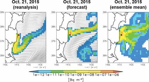
Figure 10. Surface Cs-137 concentration (Bq m⁻³) 20 days after October 1 in 2015 in 10 ensemble simulations; vectors show surface horizontal ocean current (m s⁻¹).

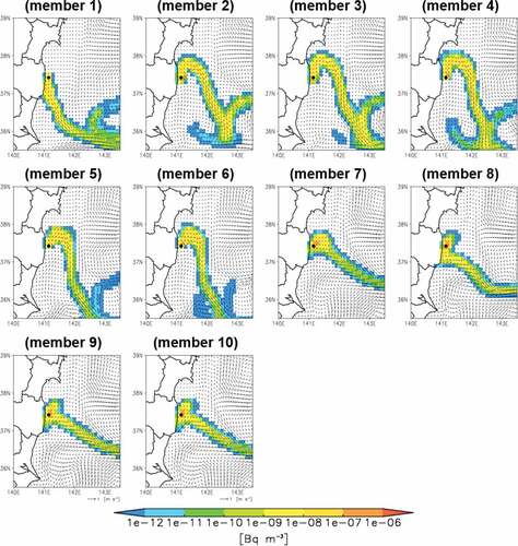
The second worst value (2%) of the predictability indicator is found for the 20-day forecast in the oceanic dispersion simulation for March 2017 (Figure 7). In this case, the reanalysis simulation shows southward Cs-137 oceanic dispersion along the coast from FNPP1 (Figure 11). Overall, the surface Cs-137 spreads only in the narrow coastal region. However, the forecast simulation shows that the surface Cs-137 disperses to the northeast from FNPP1 in the coastal region and then disperses to the southeast in the offshore region. This is mainly caused by the predictability of oceanic condition at the release point. The 10 ensemble members show an overall southeastward oceanic dispersion for Cs-137 in the offshore region, although there are variations in the dispersion patterns in the coastal region near FNPP1 among the ensemble members (Figure 12). As observed in the reanalysis simulation, member 1 shows southward Cs-137 oceanic dispersion along the coast from FNPP1, although the Cs-137 oceanic dispersion in the offshore region is different from that in the reanalysis simulation. Members 7, 8, 9, and 10 show slightly southward Cs-137 oceanic dispersion along the coast from FNPP1. As a result, the ensemble mean value of the surface Cs-137 concentration is improved over that found from the forecast simulation, especially in the coastal region south of FNPP1 (Figure 11).

Figure 11. Surface Cs-137 concentration (Bq m⁻³) 20 days after March 1 in 2017; all other notations are the same as those shown in Figure 9.

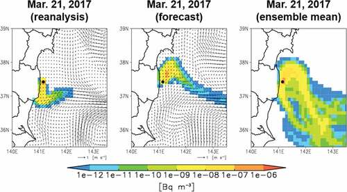
Figure 12. Surface Cs-137 concentration (Bq m⁻³) 20 days after March 1 in 2017 in 10 ensemble simulations; all other notations are the same as those shown in Figure 10.

The predictability of the Cs-137 oceanic dispersion due to the ensemble forecast simulation is quantitatively examined using the ensemble mean results. As in the forecast simulation, the predictability indicator, which is described in subsection 3.1, for the ensemble forecast simulation decreases with the forecast period (Figure 7). Overall, the ensemble forecast simulation quantitatively improves the predictability indicator for the 5-day, 10-day, 15-day, and 20-day forecasts compared with the forecast simulation, although sometimes the predictability indicator worsens. The mean predictability indicator over the period from 2015 to 2017 from the ensemble forecast simulation clearly demonstrates an improvement in the predictability of the Cs-137 oceanic dispersion over that from the forecast simulation (Figure 8). The mean predictability indicators for the period from 2015 to 2017 from the ensemble forecast simulation are calculated to be 68%, 55%, 50%, and 40% for the 5-day, 10-day, 15-day, and 20-day forecasts.

4. Conclusion

STEAMER has been developed at JAEA to forecast or reanalyze the oceanic dispersion of radionuclides released from nuclear facilities during operation or in an emergency. In this study, the predictability of STEAMER is validated by utilizing oceanographic forecast and reanalysis data that has been saved for the period from 2015 to 2017. Quantitative examination of the predictability of the oceanic dispersion of Cs-137 shows that the predictability of the oceanic dispersion decreases with the length of the forecast period. The predictability of STEAMER needs to be improved for future regular operation. In this study, ensemble forecast simulations are performed employing LAF methodology as one measure of improving the predictability of STEAMER. The ensemble forecast simulations successfully improve the predictability of the Cs-137 oceanic dispersion over that obtained from the forecast simulation.

Further validation of the predictability of STEAMER is desirable utilizing oceanographic forecast and reanalysis data that will be saved in the future. In addition, the predictability of STEAMER needs to be validated for radionuclides released from nuclear facilities other than FNPP1. Meanwhile, a sophisticated forecast methodology, such as the ensemble forecast simulation, needs to be installed in STEAMER for future regular operation. A downscale methodology also needs to be installed in STEAMER for operation to simulate the oceanic condition in the coastal region accurately. STEAMER can provide useful information on the oceanic dispersion of radionuclides in the future.

Acknowledgments

The authors thank Dr. Masafumi Kamachi of the Japan Agency for Marine-Earth Science and Technology for his support in developing STEAMER. The authors also thank Dr. Norihisa Usui of MRI of JMA for his technical support in analyzing the oceanographic data of MOVE/MRI.COM. We are also grateful to Dr. Haruyasu Nagai for his helpful advice in analyzing the simulation results.

Disclosure statement

No potential conflict of interest was reported by the authors.

References

- Aoyama M, Hirose K, Igarashi Y. Re-construction and updating our understanding on the global weapons tests 137Cs fallout. J Environ Monit. 2006;8:431–438.
- Tsumune D, Aoyama M, Hirose K, et al. Transport of 137Cs to the Southern hemisphere in an ocean general circulation model. Prog Oceanogr. 2011;89:38–48.
- Duffa C, Bailly Du Bois P, Caillaud M, et al. Development of emergency response tools for accidental radiological contamination of French coastal areas. J Envion Radioact. 2016;151:487–494.
- Kobayashi T, Kawamura H, Fujii K, et al. Development of a short-term emergency assessment system of the marine environmental radioactivity around Japan. J Nucl Sci Technol. 2017;54:609–616.
- Kobayashi T, Otosaka S, Togawa O, et al. Development of a non-conservative radionuclides dispersion model in the ocean and its application to surface cesium-137 dispersion in the Irish sea. J Nucl Sci Technol. 2007;44:238–247.
- Kamidaira Y, Kawamura H, Kobayashi T, et al. Development of regional downscaling capability in STEAMER ocean prediction system based on multi-nested ROMS model. J Nucl Sci Technol. 2019;56:752–763.
- Kawamura H, Kobayashi T, Furuno A, et al. Numerical simulation on the long-term variation of radioactive cesium concentration in the North Pacific due to the Fukushima disaster. J Environ Radioact. 2014;136:64–75.
- Kawamura H, Furuno A, Kobayashi T, et al. Oceanic dispersion of Fukushima-derived Cs-137 simulated by multiple oceanic general circulation models. J Environ Radioact. 2017;180:36–58.
- Tolman HL, Garraffo Z, Mehra A, et al. Ocean plume and tracer modeling for the Fukushima Dai’ichi event: particle tracking. In: MMAB/EMC/NOAA Tech. note. National Oceanic and Atmospheric Administration; 2013. No. 309 and p. 111.
- Usui N, Ishizaki S, Fujii Y, et al. Meteorological research institute multivariate ocean variational estimation (MOVE) system: some early results. Adv Spa Res. 2006;37:806–822.
- Ishikawa I, Tsujino H, Hirabara M, et al. Meteorological Research Institute Community Ocean Model (MRI.COM) manual. Tsukuba (Japan): Meteorological Research Institute; 2005, (Technical Reports of the Meteorological Research Institute No.47) [in Japanese].
- Smagorinsky J, Manabe S, Holloway JL. Numerical results from a nine-level general circulation model of the atmosphere. Mon Weather Rev. 1965;93:727–768.
- Miyoshi T, Kondo K, Terasaki K. Big ensemble data assimilation in numerical weather prediction. Computer. 2015;48:15–21.
- Hoffman RN, Kalnay E. Lagged average forecasting, an alternative to Monte Carlo forecasting. Tellus. 1983;35A:100–118.
- Yasuda I. Hydrographic structure and variability in the Kuroshio-Oyashio transition area. J Oceanogr. 2003;59:389–402.
- Behrens E, Schwarzkopf FU, Lübbecke JF, et al. Model simulations on the long-term dispersal of 137Cs released into the Pacific Ocean off Fukushima. Environ Res Lett. 2012;7:034004(10pp).
- Kamidaira Y, Uchiyama Y, Kawamura H, et al. Submesoscale mixing on initial dilution of radionuclides released from the Fukushima Daiichi nuclear power plant. J Geophy Res Oceans. 2018;123:2808–2828.
- Kawamura H, Kobayashi T, Furuno A, et al. Preliminary numerical experiments on oceanic dispersion of 131I and 137Cs discharged into the ocean because of the Fukushima Daiichi nuclear power plant disaster. J Nucl Sci Technol. 2011;48:1349–1356.
- Miyazawa Y, Masumoto Y, Varlamov SM, et al. Transport simulation of the radionuclide from the shelf to open ocean around Fukushima. Cont Shelf Res. 2012;50–51:16–29.