Statistical arguments towards the development of an advanced embrittlement correlation method for reactor pressure vessel materials

ABSTRACT

An embrittlement correlation method is one of the most important techniques used to ensure the integrity of pressure vessel steels in nuclear power plants. In Japan, the embrittlement correlation method is being addressed in accordance with the Japan Electric Association Code (JEAC 4201), which was developed using actual measured data on the irradiation embrittlement of pressure vessel steels. In the present study, to develop more reliable methodologies, statistical arguments were made concerning the embrittlement data. With regard to a set of residual data defined in JEAC 4201 as a collection of differences between the measured and calculated $\mathrm{\Delta }\mathrm{D}\mathrm{B}\mathrm{T}\mathrm{T}$ (ductile-to-brittle transition temperature shift) values, a statistical relationship between the population and samples was found, and then, the sampling errors in the mean values of the residuals were identified as key for establishing a more reliable correlation method. Using this relationship, it was noted that when predicting the amount of irradiation embrittlement for a particular plant using the JEAC 4201 correlation method, the deviation associated with sampling errors needed to be corrected. Based on this finding, a more appropriate interpretation was found for the so-called MC correction in JEAC 4201, and moreover, a new correction method was developed within the Bayesian estimation framework.

KEYWORDS:

• Radiation damage
• calculation
• database
• error
• LWR type reactor
• neutron irradiation
• numerical analysis

1. Irradiation embrittlement of LWR pressure vessel steels

Pressure vessel steels of ageing light water reactors (LWRs) are embrittled under the influence of neutron irradiation [1–7]. The degree of irradiation embrittlement is generally indicated by the amount of increase in the ductile-to-brittle transition temperature (DBTT) [8]. The increase in the DBTT is monitored under a surveillance program by using test specimens that have been loaded in advance into a capsule located inside the LWR pressure vessel at the start of plant operation [8]. This is one of the regulatory tasks used to confirm the integrity of pressure vessels [9–16]. The important point of this program is not only to investigate the current condition of pressure vessels but also to predict the amount of increase in the DBTT before the next monitoring opportunity.

Since the number of specimens loaded in advance at the start of operation is limited, the number of measured data obtained so far is not large and is, at most, four, even for a long-term operation plant [14–16]. Of course, it is not impossible to predict the future behavior of the target plant using the four measured data. However, from a statistical point of view, the accuracy and precision of prediction would be inadequate. To keep the accuracy and precision at or above a certain level, the number of data available for prediction should be increased.

1.1. JEAC embrittlement correlation method

The regulatory standards for maintaining the integrity of pressure vessels in commercial LWRs in Japan were established by the Japan Electric Association based on the CRIEPI embrittlement correlation model [17–21], which were coded in JEAC 4201–2007 published in 2007 [14] and its supplemented edition published in 2013 [16]. In these codes, the embrittlement correlation is described using reaction rate theory equations that are given to predict the amount of increase in the DBTT as a function of time, in which microstructural changes in pressure vessel steels due to irradiation and the corresponding DBTT changes are evaluated. Details of the equations are given in refs [14–21].

In the rate theory equations, there are 19 coefficients that should be optimized to reproduce the measured data on irradiation embrittlement of the target plant. However, considering that the number of measured data is at most four for each plant, as mentioned above, the number of coefficients is too high to determine. Therefore, when optimizing the coefficients, JEAC 4201 adopted an alternative strategy in which not only the data of the target plant but also all available data acquired from commercial LWRs in Japan and other locations were employed. The total number of data employed was approximately 400. For JEAC 4201–2007, the total number of candidate data was 419 [17], part of which was really employed; while for the supplemented edition in 2013, the total number of data employed was 371 [22].

Now, all the coefficients can be determined via this strategy. However, a new problem seems to have arisen here. It concerns data attributes such as the data characteristics, history, origin, quality, features, lineage, and properties. With regard to irradiation embrittlement, the data attributes depend on the irradiation conditions as well as the material conditions. Irradiation conditions such as the incident neutron flux and irradiation temperature vary greatly depending on the rector type, which can be pressurized water reactors (PWRs) or boiling water reactors (BWRs). Even for the same reactor type, the irradiation conditions differ to some extent from one reactor to another. In addition, the material conditions such as the chemical composition and impurity content of pressure vessel steels also depend on individual reactors. That is, collecting more data from various reactors according to the above strategy will result in greater variability of the data attributes, which will have a greater impact on the accuracy and precision of prediction. This effect must be noted when using the rate equations constructed by using approximately 400 various pieces of data.

1.2. Accuracy and precision of JEAC embrittlement correlation

Consider the accuracy and precision of the embrittlement correlation employed by JEAC 4201. Figure 1 shows a relationship between the measured amount of increase in the DBTT ($\mathrm{\Delta }\mathrm{D}\mathrm{B}\mathrm{T}{\mathrm{T}}_{\mathrm{m}\mathrm{e}\mathrm{a}}$) and the value calculated using the JEAC 4201 rate equations ($\mathrm{\Delta }\mathrm{D}\mathrm{B}\mathrm{T}{\mathrm{T}}_{\mathrm{c}\mathrm{a}\mathrm{l}}$) [18]. Approximately 400 data points appear in this figure. The solid straight line drawn diagonally in the figure indicates that the calculated value is in complete agreement with the measured value. It can be clearly seen that most of the data points are localized near the line. Now, to investigate the difference between the measured and calculated values, let us define a residual as

(1) $a=\mathrm{\Delta }\mathrm{D}\mathrm{B}\mathrm{T}{\mathrm{T}}_{\mathrm{m}\mathrm{e}\mathrm{a}}-\mathrm{\Delta }\mathrm{D}\mathrm{B}\mathrm{T}{\mathrm{T}}_{\mathrm{c}\mathrm{a}\mathrm{l}}$(1)

Figure 1. Correlation between the measured amount of increase in DBTT ($\mathrm{\Delta }\mathrm{D}\mathrm{B}\mathrm{T}{\mathrm{T}}_{\mathrm{m}\mathrm{e}\mathrm{a}}$) and the value calculated using the JEAC 4201 irradiation correlation model. The plot is reconstructed using Fig. 41(b) of ref [18]

The magnitude and sign of the residual can be recognized by the distance and relative position of the data point from the solid straight line. Although the residuals take on various values, it is interesting to note that they remain within the range of about $\pm 20$°C, as indicated by the dashed lines in the figure, and are independent of the amount of increase in the DBTT.

The figure additionally indicates that there are 13 data points not included in the range. These data points seem to be extraordinary, but they are only 3–4% of the total. According to refs [18,19,22], the residual data have the mean values of ${\mu }_0=0.1$°C for JEAC 4201–2007 and of ${\mu }_0=-1.11$°C for the supplemented edition in 2013. The observed mean values of ${\mu }_0\approx 0$°C are quite reasonable and are consistent with the fact that ${\mu }_0$ should ideally be zero because the coefficients of the rate equations were determined by optimization using the measured data, as mentioned above. On the other hand, the standard deviations are reported as ${\sigma }_0=9.4$°C for JEAC 4201–2007 and ${\sigma }_0=9.47$°C [18,22] for the supplemented edition in 2013, which indicate that the range of $\pm 20$°C mentioned above is almost equivalent to $\pm 2{\sigma }_0$. Roughly speaking, if the residual data obey the normal probability distribution, it is not completely unreasonable that the 13 data points are plotted outside the range because approximately 5% of the total are statistically outside the range of $\pm 2{\sigma }_0$ of the normal probability distribution.

It is known from a statistical point of view that there are two types of errors: one is random error, and the other is systematic error. Systematic error produces the fluctuation of data values, depending on such parameters as the neutron flux, temperature, chemical composition, etc., whereas random error is statistical variability that inevitably appears and generally obeys the normal probability distribution. According to refs [21,22], it is reported that the average behavior of approximately 400 residual data in JEAC 4201 do not depend on any irradiation or material conditions such as the neutron flux, temperature, and chemical composition. Rather, it may be more accurate to state that the coefficients of the rate theory equations have been determined so that dependencies do not appear to the extent possible. Regardless, this may indicate that dependencies on those conditions are all successfully included within a description of the rate theory equations. Thus, the residuals only contain the component of random errors. The residual data defined above appear to show only the behavior of random noise, and hence, it is hereinafter assumed that the residual can be well described by the normal probability distribution. This characteristic of the residual data is very useful later when considering the correction method used to improve the accuracy of the prediction.

It is noted that the above discussion on the distribution of residual data is for about all 400 data represented in Figure 1. Needless to say, the distribution of residual data can also be defined individually at each plant. Unfortunately, however, the current JEAC 4201 [14–16] does not mention the distributions of individual plants at all. This is probably because the number of data obtained at each plant is only four at most, which is too few to discuss the distribution and statistics of each plant. This is indeed reasonable. However, the lack of this argument may be the reason why the irradiation embrittlement of each plant cannot seem to be predicted with sufficient accuracy, as discussed later.

1.3. Application of the JEAC 4201 embrittlement correlation method to individual plants

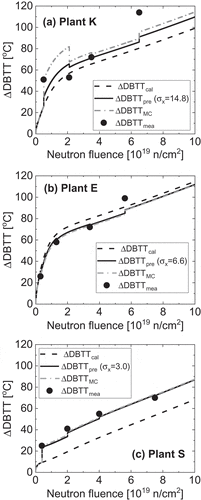
Now, let us look at some examples. Figure 2 shows the time evolution of the amount of increase in the DBTT for plant K [23], E [24], and S [25]. Note that K, E, and S are the names of ageing PWR plants that actually exist in Japan, and the number of surveillance tests is four for each plant. The figures show that the measured data points and the calculated curve are represented by dots and a dashed line, respectively. As shown in the figures, the magnitude of the residuals is different depending on the plant, which may indicate a plant-specific property. For example, in plant E [24], the calculated curve seems to be almost in agreement with the measured values. In plant S [25], on the other hand, the residuals seem to take on a systematic bias. If so, the above conclusion that the residuals of JEAC 4201 contain no systematic errors may become doubtful. Furthermore, in plant K [23], the residuals exhibit large fluctuations.

Figure 2. Time evolutions of the amount of increase in DBTT for (a) plant K, (b) plant E, and (c) plant S [23–25]. All of the plants are PWRs that actually exist in Japan

When looking at the examples more closely, it is found that all the four measured data points are higher than the calculated curve in plant S [24], while they are all lower in plant E [25]. It is reported in ref [22]. that there are quite a few cases in which all measured data are above or below the calculated values, as in the cases of plant S and plant E. Needless to say, statistically, the fraction of such cases should be ${\left(1/2\right)}^4$= 6.25% of the total, but in fact, the observed fractions of those plants are as high as 24.4% and 19.5%, respectively [22]. From this finding, it may seem that there is a bias in many cases; however, this obviously contradicts the above conclusion that bias should essentially not occur because residuals contain only random errors. Is there actually a bias? Or is it just an appearance?

Aside from the question of the credibility of the existence of bias, let us look at the practical solution that JEAC 4201 has adopted, wherein the ‘bias’ seen here was compensated by the methodology called MC correction. This could be the so-called ‘engineering judgement’ that was adopted by JEAC 4201 from the viewpoint of plant safety.

In the MC correction, an Mc value is first evaluated using the measured data that have been obtained at the target plant X, as follows:

(2) $\mathrm{M}\mathrm{c}=\frac{1}{N_X}{\sum }_{i=1}^{N_X}\left\{\mathrm{\Delta }\mathrm{D}\mathrm{B}\mathrm{T}{\mathrm{T}}_{\mathrm{m}\mathrm{e}\mathrm{a}}\left(t_i\right)-\mathrm{\Delta }\mathrm{D}\mathrm{B}\mathrm{T}{\mathrm{T}}_{\mathrm{c}\mathrm{a}\mathrm{l}}\left(t_i\right)\right\},$(2)

where i indicates the order of the measurements and is an integer from 1 to $N_X$. $N_X$ is the maximum number of measurements, which takes only four at most, even in the case of long-term operating plants aged over 40 years. $\mathrm{\Delta }\mathrm{D}\mathrm{B}\mathrm{T}{\mathrm{T}}_{\mathrm{m}\mathrm{e}\mathrm{a}}\left(t_i\right)$ and $\mathrm{\Delta }\mathrm{D}\mathrm{B}\mathrm{T}{\mathrm{T}}_{\mathrm{c}\mathrm{a}\mathrm{l}}\left(t_i\right)$ are the measured and calculated DBTT shifts at time $t_i$, respectively. Then, the $M_{\mathrm{C}}$ value evaluated is added to the JEAC 4201 calculated value, and finally, the corrected value is given by

(3) $\mathrm{\Delta }\mathrm{D}\mathrm{B}\mathrm{T}{\mathrm{T}}_{\mathrm{M}\mathrm{C}}=\mathrm{\Delta }\mathrm{D}\mathrm{B}\mathrm{T}{\mathrm{T}}_{\mathrm{c}\mathrm{a}\mathrm{l}}+M_{\mathrm{C}}$(3)

In Figure 2, the $\mathrm{\Delta }\mathrm{D}\mathrm{B}\mathrm{T}{\mathrm{T}}_{\mathrm{M}\mathrm{C}}$ curves are also drawn as solid curves. The solid curves seem to represent the average behavior of the measured data points very well, indicating that the correction works well. However, is this interpretation correct? More attention must be paid here. Taking into consideration the fact that the $M_{\mathrm{C}}$ value defined by Equation (2)(2) $\mathrm{M}\mathrm{c}=\frac{1}{N_X}{\sum }_{i=1}^{N_X}\left\{\mathrm{\Delta }\mathrm{D}\mathrm{B}\mathrm{T}{\mathrm{T}}_{\mathrm{m}\mathrm{e}\mathrm{a}}\left(t_i\right)-\mathrm{\Delta }\mathrm{D}\mathrm{B}\mathrm{T}{\mathrm{T}}_{\mathrm{c}\mathrm{a}\mathrm{l}}\left(t_i\right)\right\},$(2) is the average of the residuals, it seems to be neither wonder nor coincidental that the corrected curve represents the average behavior of the data points well. Ironically, such a method of correction seems to be only a hindsight trick. Is the MC correction really valid from the aspect of physics?

According to JEAC 4201 [14], the MC correction represented by Equation (3)(3) $\mathrm{\Delta }\mathrm{D}\mathrm{B}\mathrm{T}{\mathrm{T}}_{\mathrm{M}\mathrm{C}}=\mathrm{\Delta }\mathrm{D}\mathrm{B}\mathrm{T}{\mathrm{T}}_{\mathrm{c}\mathrm{a}\mathrm{l}}+M_{\mathrm{C}}$(3) was proposed to compensate for the ambiguity of initial $\mathrm{D}\mathrm{B}\mathrm{T}\mathrm{T}$ values. Certainly, the initial values are different depending on the test specimens, and therefore, there is a need to discuss the ambiguity of the initial values. However, unfortunately, there is no guarantee that this ambiguity is in agreement with the Mc value defined above. To validate the MC correction method, additional explanations are needed.

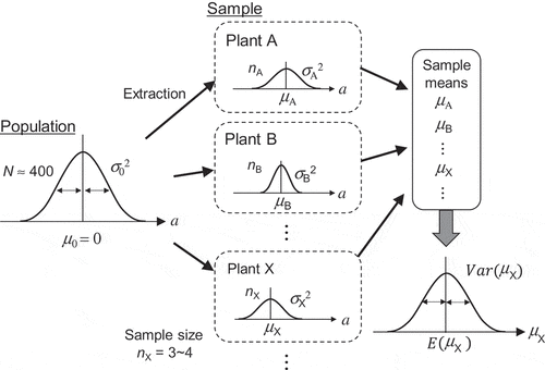
In the present study, based on the arguments presented so far, theoretical evaluations were conducted. The statistical sampling theory dealing with the relationship between populations and samples was applied to obtain the statistical properties of the residual data defined above, in which the residuals were employed as variables of a population. The residual data of each plant were regarded as samples extracted from the population. This situation is schematically drawn in Figure 3. In this viewpoint, the central limit theorem and large number theorem of statistics [26–28] were applied to discuss the relationship. In the next section, the statistical theorem and approaches are presented. In the section 3, the interpretation of MC correction is revised, followed by the development of a new methodology within the framework of Bayesian statistics. Finally, conclusions are given in section 4.

Figure 3. Schematic representation of the relationship between the population and samples

2. Theory

In this work, the statistical sampling theory dealing with the relationship between a population and samples was applied, in which two limit theorems [26–28], i.e. the central limit theorem (CLT) and the law of large numbers, were used. With these theorems, the statistical property of the residual data was first investigated.

The Bayesian updating method was then applied to construct a more reliable embrittlement correlation. The probability density distribution function $\pi$ was defined with respect to the data D and the parameter $\mu$, and then using the Bayesian theorem [26–28], the posterior probability density distribution function of $\mu$ for $\mathrm{a}$ given D was written as

(4) $\pi \left(\mu |D\right)\propto f\left(D|\mu \right)\cdot \pi \left(\mu \right)$(4)

where $\pi \left(\mu \right)$ is the prior probability density distribution function of $\mu$ and $f\left(D|\mu \right)$ is the likelihood of D for a given $\mu$. Using this expression, the probability density function π of μ was updated each time data D was newly obtained. For the data D in Equation (4)(4) $\pi \left(\mu |D\right)\propto f\left(D|\mu \right)\cdot \pi \left(\mu \right)$(4) , the residuals a were employed.

3. Results and discussion

3.1. Statistical consideration of irradiation embrittlement data in JEAC 4201

In JEAC 4201, a set of rate equations was constructed, as mentioned above, using approximately 400 pieces of actual measured embrittlement data. Strictly speaking, the subject here is not the measured embrittlement data itself but the residuals, i.e. the differences between the measured and calculated DBTT values. As noted above, the residuals are associated with only random errors that obey the normal probability distribution with the mean ${\mu }_0$ and the standard deviation ${\sigma }_0$. In this study, the residuals were regarded as statistical variables of a finite population. Needless to say, the residuals obtained at each plant are variables of a small subset of this population. Thus, the residual data of each plant can be regarded as samples drawn from the population, as shown in Figure 3. This relationship between the population and samples will be the basis for the discussions below.

It is obviously found from Equations (1)(1) $a=\mathrm{\Delta }\mathrm{D}\mathrm{B}\mathrm{T}{\mathrm{T}}_{\mathrm{m}\mathrm{e}\mathrm{a}}-\mathrm{\Delta }\mathrm{D}\mathrm{B}\mathrm{T}{\mathrm{T}}_{\mathrm{c}\mathrm{a}\mathrm{l}}$(1) and (2(2) $\mathrm{M}\mathrm{c}=\frac{1}{N_X}{\sum }_{i=1}^{N_X}\left\{\mathrm{\Delta }\mathrm{D}\mathrm{B}\mathrm{T}{\mathrm{T}}_{\mathrm{m}\mathrm{e}\mathrm{a}}\left(t_i\right)-\mathrm{\Delta }\mathrm{D}\mathrm{B}\mathrm{T}{\mathrm{T}}_{\mathrm{c}\mathrm{a}\mathrm{l}}\left(t_i\right)\right\},$(2) ) that the Mc value is merely the mean of the residual data obtained in each plant. When considering the population-sample relationship above, the Mc value of plant X can be regarded as the ‘sample mean’, which is hereafter depicted as ${\mu }_X$. Upon applying the law of large numbers of statistics [26–28], the mean of the Mc values of all plants must be $0$°C because the mean of the sample means agrees with the population mean. Additionally, by using the central limit theorem of statistics [26–28], the standard deviation of the distribution of the Mc values, i.e. the standard error of the sample means, is given by

(5) $Std\left({\mu }_X\right)=\sqrt{\frac{N-N_X}{N-1}\cdot \frac{{\sigma }_0^2}{N_X}}$(5)

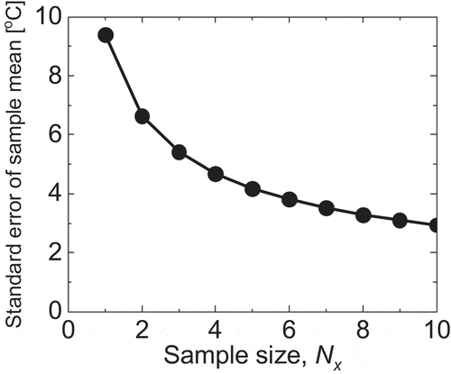
where N is the number of data in the finite population and $N_X$ is the sample size. Figure 4 shows the standard error of the sample mean calculated by Equation (5)(5) $Std\left({\mu }_X\right)=\sqrt{\frac{N-N_X}{N-1}\cdot \frac{{\sigma }_0^2}{N_X}}$(5) when the population standard deviation is set to ${\sigma }_0=9.4$°C (JEAC 4201–2007). Since JEAC 4201–2007 was published in 2007, $N_X$ is considered to be nearly three. Therefore, when $N_X=3$ is applied to Equation (5)(5) $Std\left({\mu }_X\right)=\sqrt{\frac{N-N_X}{N-1}\cdot \frac{{\sigma }_0^2}{N_X}}$(5) and Figure 4, $Std\left({\mu }_X\right)$ in Equation (5)(5) $Std\left({\mu }_X\right)=\sqrt{\frac{N-N_X}{N-1}\cdot \frac{{\sigma }_0^2}{N_X}}$(5) is estimated to be $5.4$°C.

Figure 4. Standard error of the sample mean calculated by Equation (5)(5) $Std\left({\mu }_X\right)=\sqrt{\frac{N-N_X}{N-1}\cdot \frac{{\sigma }_0^2}{N_X}}$(5) when ${\sigma }_0=9.4$°C is applied

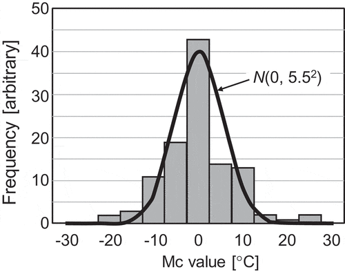
Figure 5 shows the distribution of Mc values in JEAC 4201–2007, which was reported in ref [29]. The figure indicates that the mean of this distribution is $0$°C and the standard deviation is $5.5$°C. These two values are in good agreement with the population mean ${\mu }_0=0$°C and the estimated standard error $5.4$°C, respectively. The consistencies of the two values indicate that there is no contradiction of the concept that the relationship between the population and sample discussed above is valid. Based on this concept, a prediction of the irradiation embrittlement for a particular plant is made as shown below.

Figure 5. Distribution of the Mc values in JEAC 4201–2007, indicating a normal probability distribution with a mean of $0$°C and standard deviation of $5.5$°C.

3.2. Revisit of the interpretation of MC correction

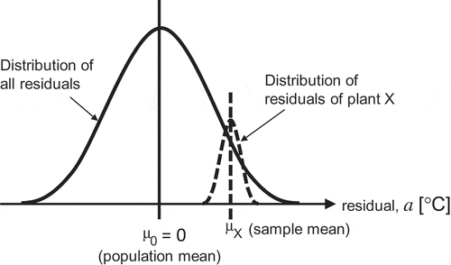
In this section, the accuracy and precision of the embrittlement correlation including the validity of the MC correction are discussed using the population-sample relationship identified above. Figure 6 is a schematic representation showing the distributions of the population on residuals for all plants and of the small subset for plant X. Both distributions naturally take the form of a normal probability distribution because the residuals do not include systematic errors, but they do not necessarily match one another, indicating that the distribution is plant-specific. That is, even random errors must be plant-dependent. The deviation of the two distributions is the essential reason why the correction is needed and is indexed by the differences between their mean values (${\delta }_X={\mu }_X-{\mu }_0$), which is usually referred to as the sampling error about the mean.

Figure 6. Schematic representation of the distribution of all residuals and those of plant X. Both distributions have the form of a normal probability distribution. It is noted that the residuals do not include the component of systematic errors, but their distributions are plant-specific

Let us look at Equation (1)(1) $a=\mathrm{\Delta }\mathrm{D}\mathrm{B}\mathrm{T}{\mathrm{T}}_{\mathrm{m}\mathrm{e}\mathrm{a}}-\mathrm{\Delta }\mathrm{D}\mathrm{B}\mathrm{T}{\mathrm{T}}_{\mathrm{c}\mathrm{a}\mathrm{l}}$(1) again, showing that the measured value deviates from the calculated value by $a$. Considering that $\mathrm{\Delta }\mathrm{D}\mathrm{B}\mathrm{T}{\mathrm{T}}_{\mathrm{m}\mathrm{e}\mathrm{a}}$ is the target value to be predicted, the predicted value $\mathrm{\Delta }\mathrm{D}\mathrm{B}\mathrm{T}{\mathrm{T}}_{\mathrm{p}\mathrm{r}\mathrm{e}}$ is then given by

(6) $\mathrm{\Delta }\mathrm{D}\mathrm{B}\mathrm{T}{\mathrm{T}}_{\mathrm{p}\mathrm{r}\mathrm{e}}=\mathrm{\Delta }\mathrm{D}\mathrm{B}\mathrm{T}{\mathrm{T}}_{\mathrm{c}\mathrm{a}\mathrm{l}}+a$(6)

which is obtained by simply replacing $\mathrm{\Delta }\mathrm{D}\mathrm{B}\mathrm{T}{\mathrm{T}}_{\mathrm{m}\mathrm{e}\mathrm{a}}$ in Equation (1)(1) $a=\mathrm{\Delta }\mathrm{D}\mathrm{B}\mathrm{T}{\mathrm{T}}_{\mathrm{m}\mathrm{e}\mathrm{a}}-\mathrm{\Delta }\mathrm{D}\mathrm{B}\mathrm{T}{\mathrm{T}}_{\mathrm{c}\mathrm{a}\mathrm{l}}$(1) with $\mathrm{\Delta }\mathrm{D}\mathrm{B}\mathrm{T}{\mathrm{T}}_{\mathrm{p}\mathrm{r}\mathrm{e}}$. The parameter $a$ obeys the normal probability distribution $N\left({\mu }_0,{\sigma }_0^2\right)$, as mentioned above. Since ${\mu }_0=0$, $\mathrm{\Delta }\mathrm{D}\mathrm{B}\mathrm{T}{\mathrm{T}}_{\mathrm{p}\mathrm{r}\mathrm{e}}$ matches $\mathrm{\Delta }\mathrm{D}\mathrm{B}\mathrm{T}{\mathrm{T}}_{\mathrm{c}\mathrm{a}\mathrm{l}}$ on average. In addition, the last term in Equation (6)(6) $\mathrm{\Delta }\mathrm{D}\mathrm{B}\mathrm{T}{\mathrm{T}}_{\mathrm{p}\mathrm{r}\mathrm{e}}=\mathrm{\Delta }\mathrm{D}\mathrm{B}\mathrm{T}{\mathrm{T}}_{\mathrm{c}\mathrm{a}\mathrm{l}}+a$(6) represents the ambiguity of the predicted value, which is described by the standard deviation ${\sigma }_0$. These attributes are what Equation (6)(6) $\mathrm{\Delta }\mathrm{D}\mathrm{B}\mathrm{T}{\mathrm{T}}_{\mathrm{p}\mathrm{r}\mathrm{e}}=\mathrm{\Delta }\mathrm{D}\mathrm{B}\mathrm{T}{\mathrm{T}}_{\mathrm{c}\mathrm{a}\mathrm{l}}+a$(6) implies. This implication is equivalent to the methodology adopted by JEAC 4201, in which the value to be predicted is first given by solving the rate equations (i.e. $\mathrm{\Delta }\mathrm{D}\mathrm{B}\mathrm{T}{\mathrm{T}}_{\mathrm{p}\mathrm{r}\mathrm{e}}=\mathrm{\Delta }\mathrm{D}\mathrm{B}\mathrm{T}{\mathrm{T}}_{\mathrm{c}\mathrm{a}\mathrm{l}}$), and then the population standard deviation ${\sigma }_0$ is employed to define the margin (i.e. $M_{\mathrm{R}}=2{\sigma }_0$) [14,16].

Unfortunately, however, this methodology and interpretation could not produce a prediction with sufficient accuracy and precision, as seen in the case of plant S. Therefore, JEAC 4201 additionally adopted the MC correction method shown in Equation (3)(3) $\mathrm{\Delta }\mathrm{D}\mathrm{B}\mathrm{T}{\mathrm{T}}_{\mathrm{M}\mathrm{C}}=\mathrm{\Delta }\mathrm{D}\mathrm{B}\mathrm{T}{\mathrm{T}}_{\mathrm{c}\mathrm{a}\mathrm{l}}+M_{\mathrm{C}}$(3) , but this method is obviously beyond the implications of Equation (6)(6) $\mathrm{\Delta }\mathrm{D}\mathrm{B}\mathrm{T}{\mathrm{T}}_{\mathrm{p}\mathrm{r}\mathrm{e}}=\mathrm{\Delta }\mathrm{D}\mathrm{B}\mathrm{T}{\mathrm{T}}_{\mathrm{c}\mathrm{a}\mathrm{l}}+a$(6) and seems to be a hindsight trick.

Consider the distribution of the parameter $a$ in Equation (6)(6) $\mathrm{\Delta }\mathrm{D}\mathrm{B}\mathrm{T}{\mathrm{T}}_{\mathrm{p}\mathrm{r}\mathrm{e}}=\mathrm{\Delta }\mathrm{D}\mathrm{B}\mathrm{T}{\mathrm{T}}_{\mathrm{c}\mathrm{a}\mathrm{l}}+a$(6) again. Indeed, as mentioned above, the parameter $a$ obeys $N\left(0,{\sigma }_0^2\right)$. However, we must be careful of the fact that the distribution of parameter $a$ was constructed using about all 400 data sets, which contain a wide variety of data in addition to that of the target plant to be predicted. Obviously, variation in the data attributes will make it difficult to predict the behavior of target plants with sufficient accuracy and precision. Therefore, we would like to propose taking a value of $a$ in Equation (6)(6) $\mathrm{\Delta }\mathrm{D}\mathrm{B}\mathrm{T}{\mathrm{T}}_{\mathrm{p}\mathrm{r}\mathrm{e}}=\mathrm{\Delta }\mathrm{D}\mathrm{B}\mathrm{T}{\mathrm{T}}_{\mathrm{c}\mathrm{a}\mathrm{l}}+a$(6) not from $N\left(0,{\sigma }_0^2\right)$ but from $N\left({\mu }_X,{\sigma }_X^2\right)$, where ${\sigma }_X$ is the standard deviation of the residuals for the target plant X. Since $N\left({\mu }_X,{\sigma }_X^2\right)$ is a plant-specific distribution, this attempt will produce a more accurate and precise embrittlement correlation for a particular plant.

Let us define the values ${\xi }_X$ and ${\xi }_0$, which obey the normal probability distributions $N\left({\mu }_X,{\sigma }_X^2\right)$ and $N\left(0,{\sigma }_X^2\right)$, respectively. Regarding these two values, we can find a useful relationship:

(7) ${\xi }_X={\xi }_0+{\mu }_X$(7)

When a value of $a$ in Equation (6)(6) $\mathrm{\Delta }\mathrm{D}\mathrm{B}\mathrm{T}{\mathrm{T}}_{\mathrm{p}\mathrm{r}\mathrm{e}}=\mathrm{\Delta }\mathrm{D}\mathrm{B}\mathrm{T}{\mathrm{T}}_{\mathrm{c}\mathrm{a}\mathrm{l}}+a$(6) is replaced by ${\xi }_X$ and Equation (7)(7) ${\xi }_X={\xi }_0+{\mu }_X$(7) is applied, then we may obtain

(8) $\mathrm{\Delta }\mathrm{D}\mathrm{B}\mathrm{T}{\mathrm{T}}_{\mathrm{p}\mathrm{r}\mathrm{e}}=\left(\mathrm{\Delta }\mathrm{D}\mathrm{B}\mathrm{T}{\mathrm{T}}_{\mathrm{c}\mathrm{a}\mathrm{l}}+{\mu }_X\right)+{\xi }_0$(8)

Upon applying a similar method to the interpretation of Equation (6)(6) $\mathrm{\Delta }\mathrm{D}\mathrm{B}\mathrm{T}{\mathrm{T}}_{\mathrm{p}\mathrm{r}\mathrm{e}}=\mathrm{\Delta }\mathrm{D}\mathrm{B}\mathrm{T}{\mathrm{T}}_{\mathrm{c}\mathrm{a}\mathrm{l}}+a$(6) , this equation indicates that the predicted value is $\mathrm{\Delta }\mathrm{D}\mathrm{B}\mathrm{T}{\mathrm{T}}_{\mathrm{c}\mathrm{a}\mathrm{l}}+{\mu }_X$, on average, and its ambiguity is given by ${\xi }_0\sim N\left(0,{\sigma }_X^2\right)$. With this implication, the margin $M_{\mathrm{R}}$ should be given by ${\sigma }_{\mathrm{X}}$.

Now, revisit the validity of the MC correction. $M\mathrm{c}$ is defined as the mean value of the residuals obtained in each plant, and hence, it is exactly the same as ${\mu }_X$ for plant X. Then, when ${\mu }_X$ in Equation (8)(8) $\mathrm{\Delta }\mathrm{D}\mathrm{B}\mathrm{T}{\mathrm{T}}_{\mathrm{p}\mathrm{r}\mathrm{e}}=\left(\mathrm{\Delta }\mathrm{D}\mathrm{B}\mathrm{T}{\mathrm{T}}_{\mathrm{c}\mathrm{a}\mathrm{l}}+{\mu }_X\right)+{\xi }_0$(8) is replaced by $M\mathrm{c}$ and Equation (3)(3) $\mathrm{\Delta }\mathrm{D}\mathrm{B}\mathrm{T}{\mathrm{T}}_{\mathrm{M}\mathrm{C}}=\mathrm{\Delta }\mathrm{D}\mathrm{B}\mathrm{T}{\mathrm{T}}_{\mathrm{c}\mathrm{a}\mathrm{l}}+M_{\mathrm{C}}$(3) is applied, we finally obtain the following equation:

(9) $\mathrm{\Delta }\mathrm{D}\mathrm{B}\mathrm{T}{\mathrm{T}}_{\mathrm{p}\mathrm{r}\mathrm{e}}=\mathrm{\Delta }\mathrm{D}\mathrm{B}\mathrm{T}{\mathrm{T}}_{\mathrm{M}\mathrm{C}}+{\xi }_0$(9)

This equation indicates that the predicted value is equivalent to $\mathrm{\Delta }\mathrm{D}\mathrm{B}\mathrm{T}{\mathrm{T}}_{\mathrm{M}\mathrm{C}}$ on average. Additionally, the ambiguity is given by ${\xi }_0\sim N\left(0,{\sigma }_X^2\right)$, wherein the margin should be $M_{\mathrm{R}}=2{\sigma }_{\mathrm{X}}$ instead of $2{\sigma }_0$. Although the expression of the ambiguity is obviously different from that of JEAC 4201, the average behavior in Equation (9)(9) $\mathrm{\Delta }\mathrm{D}\mathrm{B}\mathrm{T}{\mathrm{T}}_{\mathrm{p}\mathrm{r}\mathrm{e}}=\mathrm{\Delta }\mathrm{D}\mathrm{B}\mathrm{T}{\mathrm{T}}_{\mathrm{M}\mathrm{C}}+{\xi }_0$(9) is in agreement with that of JEAC 4201. Namely, regarding the average behavior, at least, the current MC correction is considered to be valid from the statistical viewpoint.

In summary, if the purpose is to merely know the overall behavior of all LWRs in Japan, $a$ in Equation (6)(6) $\mathrm{\Delta }\mathrm{D}\mathrm{B}\mathrm{T}{\mathrm{T}}_{\mathrm{p}\mathrm{r}\mathrm{e}}=\mathrm{\Delta }\mathrm{D}\mathrm{B}\mathrm{T}{\mathrm{T}}_{\mathrm{c}\mathrm{a}\mathrm{l}}+a$(6) needs only to obey the normal probability distribution $N\left(0,{\sigma }_0^2\right)$. This is a description of the JEAC 4201 embrittlement correlation without the MC correction. In this case, a bias-like gap as seen in plant S in Figure 2 should be accepted. Obviously, this is not our purpose. To predict the embrittlement behavior of a particular plant with sufficient accuracy and precision, $a$ in Equation (6)(6) $\mathrm{\Delta }\mathrm{D}\mathrm{B}\mathrm{T}{\mathrm{T}}_{\mathrm{p}\mathrm{r}\mathrm{e}}=\mathrm{\Delta }\mathrm{D}\mathrm{B}\mathrm{T}{\mathrm{T}}_{\mathrm{c}\mathrm{a}\mathrm{l}}+a$(6) should obey the distribution $N\left({\mu }_X,{\sigma }_X^2\right)$ defined for each plant. Since the distribution is, however, not known from the beginning, Bayesian updating is performed to estimate the distribution empirically, as described below.

3.3. Bayesian correction method

Once new DBTT data are obtained at plant X, a residual value $a^{\left(X\right)}$ is newly obtained. Upon substituting the new $a^{\left(X\right)}$ into D in the Bayesian expression in Equation (4)(4) $\pi \left(\mu |D\right)\propto f\left(D|\mu \right)\cdot \pi \left(\mu \right)$(4) , ${\mu }_X$ is updated, and then $\mathrm{\Delta }\mathrm{D}\mathrm{B}\mathrm{T}{\mathrm{T}}_{\mathrm{p}\mathrm{r}\mathrm{e}}$ is updated using Equation (8)(8) $\mathrm{\Delta }\mathrm{D}\mathrm{B}\mathrm{T}{\mathrm{T}}_{\mathrm{p}\mathrm{r}\mathrm{e}}=\left(\mathrm{\Delta }\mathrm{D}\mathrm{B}\mathrm{T}{\mathrm{T}}_{\mathrm{c}\mathrm{a}\mathrm{l}}+{\mu }_X\right)+{\xi }_0$(8) . This is hereafter called the Bayesian correction. The likelihood $f$ of the Bayesian expression in Equation (4)(4) $\pi \left(\mu |D\right)\propto f\left(D|\mu \right)\cdot \pi \left(\mu \right)$(4) indicates the probability that the data $a^{\left(X\right)}$ appears when ${\mu }_X$ is given, which is represented by

(10) $f\left(a^{\left(X\right)}|{\mu }_X\right)=\frac{1}{\sqrt{2\pi }{\sigma }_X}exp\left(-\frac{{\left(a^{\left(X\right)}-{\mu }_X\right)}^2}{2{\sigma }_X^2}\right)$(10)

The standard deviation ${\sigma }_X$ is the magnitude of the fluctuations of the residual data for plant X, which is a plant-specific property. Since this is also not known in the beginning, the population standard deviation ${\sigma }_0$ is used instead for the time being, until the actual measured data are sufficiently accumulated to evaluate ${\sigma }_X$. Fortunately, as we find later, the value of ${\mu }_X$ to be estimated does not depend much on ${\sigma }_X$.

Regarding the prior distribution π in the Bayesian expression, the distribution of the population is used as an initial distribution. Thus, we finally obtain the Bayesian expression as follows;

$\pi \left({\mu }_X|a^{\left(X\right)}\right)\propto f\left(a^{\left(X\right)}|{\mu }_X\right)\cdot \pi \left({\mu }_X\right)$

(11) $=exp\left(-\frac{{\left(a^{\left(X\right)}-{\mu }_X\right)}^2}{2{\sigma }_X^2}\right)exp\left(-\frac{{\left({\mu }_X-{\mu }_0\right)}^2}{2{\sigma }_0^2}\right)$(11)

It is found from this equation that the prior distribution π is replaced by the normal probability distribution with the mean of $\frac{{\sigma }_0^2{a}^{\left(\mathrm{X}\right)}+{\sigma }_X^2{\mu }_0}{\left({\sigma }_0^2+{\sigma }_X^2\right)}$ and the standard deviation of ${\left(\frac{1}{{\sigma }_X^2}+\frac{1}{{\sigma }_0^2}\right)}^{-\frac{1}{2}}$. This updated distribution is usually called the posterior distribution, which will become the prior distribution for the next Bayesian trial.

3.4. Application of the Bayesian correction

Now, let us apply the Bayesian correction method to some example nuclear plants K, E, and S. Table 1 shows the irradiation and material conditions for the three target plants [30], all of which actually exist in Japan. Even in the identical plants, the neutron flux is generally different, depending on the location of the surveillance test specimens installed in the pressure vessel. However, for simplicity, the value of the neutron flux used to calculate $\mathrm{\Delta }\mathrm{D}\mathrm{B}\mathrm{T}{\mathrm{T}}_{\mathrm{c}\mathrm{a}\mathrm{l}}$ was herein assumed to be a constant. The average neutron flux was employed for each plant. This simplification fortunately has no impact on the calculation results. In fact, when $\mathrm{\Delta }\mathrm{D}\mathrm{B}\mathrm{T}{\mathrm{T}}_{\mathrm{c}\mathrm{a}\mathrm{l}}$ was calculated using the JEAC rate equations for the example plants, the variation of the neutron flux indicated only a few percent in most cases. Even in the highest case, the variation was estimated to be only 27%, which corresponds to a small change of the calculated $\mathrm{\Delta }\mathrm{D}\mathrm{B}\mathrm{T}{\mathrm{T}}_{\mathrm{c}\mathrm{a}\mathrm{l}}$ of $0.4$°C, at most. Using these conditions and simplification, the DBTT changes were calculated as listed in Table 2–4. The measured values of $\mathrm{\Delta }\mathrm{D}\mathrm{B}\mathrm{T}{\mathrm{T}}_{\mathrm{m}\mathrm{e}\mathrm{a}}$ are also listed in the tables, which are exactly the values measured at the existing plants [23–25].

Table 1. Irradiation and material conditions employed as example plants. Neutron flux of each plant was obtained by using open data to the public on total neutron fluence and effective full power year (EFPY)

Plant name	Plant K	Plant E	Plant S
Cu [wt%]	0.12	0.16	0.05
Ni [wt%]	0.56	0.61	0.62
Irradiation temperature [°C]	288	288	288
Neutron flux [n/cm^2/s]	3.3 × 10^10	3.4 × 10^10	3.3 × 10^10

Table 2. Calculated results obtained from MC and Bayesian corrections for plant K

				${\sigma }_X=9.47$ [°C]		${\sigma }_X=14.8$ [°C]
Neutron fluence [n/cm^2]	$\mathrm{\Delta }\mathrm{D}\mathrm{B}\mathrm{T}{\mathrm{T}}_{\mathrm{m}\mathrm{e}\mathrm{a}}$ [°C]	$\mathrm{\Delta }\mathrm{D}\mathrm{B}\mathrm{T}{\mathrm{T}}_{\mathrm{c}\mathrm{a}\mathrm{l}}$ [°C]	$M_{\mathrm{c}}$ [°C]	${\mu }_X$[°C]	$\mathrm{\Delta }\mathrm{D}\mathrm{B}\mathrm{T}{\mathrm{T}}_{\mathrm{p}\mathrm{r}\mathrm{e}}$[°C]	${\mu }_X$[°C]	$\mathrm{\Delta }\mathrm{D}\mathrm{B}\mathrm{T}{\mathrm{T}}_{\mathrm{p}\mathrm{r}\mathrm{e}}$[°C]
0	-	-	-	0	-	0	-
0.5 × 10^19	51	25.9	25.1	12.6	38.5	7.3	33.2
2.1 × 10^19	53	56.8	10.7	7.1	63.9	4.8	61.6
3.5 × 10^19	72	65.6	9.2	6.9	72.5	5.1	70.7
6.5 × 10^19	114	80.4	15.3	12.3	92.7	9.5	89.9

Table 3. Calculated results obtained from MC and Bayesian corrections for plant E

				${\sigma }_X=9.47$ [°C]		${\sigma }_X=6.6$ [°C]
Neutron fluence [n/cm^2]	$\mathrm{\Delta }\mathrm{D}\mathrm{B}\mathrm{T}{\mathrm{T}}_{\mathrm{m}\mathrm{e}\mathrm{a}}$ [°C]	$\mathrm{\Delta }\mathrm{D}\mathrm{B}\mathrm{T}{\mathrm{T}}_{\mathrm{c}\mathrm{a}\mathrm{l}}$ [°C]	$M_{\mathrm{c}}$ [°C]	${\mu }_X$ [°C]	$\mathrm{\Delta }\mathrm{D}\mathrm{B}\mathrm{T}{\mathrm{T}}_{\mathrm{p}\mathrm{r}\mathrm{e}}$ [°C]	${\mu }_X$ [°C]	$\mathrm{\Delta }\mathrm{D}\mathrm{B}\mathrm{T}{\mathrm{T}}_{\mathrm{p}\mathrm{r}\mathrm{e}}$ [°C]
0	-	-	-	0	-	0	-
0.3 × 10^19	26	31.5	-5.5	-2.8	28.8	-3.7	27.8
1.3 × 10^19	58	65.3	-6.4	-4.3	61.0	-5.1	60.2
3.4 × 10^19	72	79.9	-6.9	-5.2	74.7	-5.9	74.0
5.6 × 10^19	99	90.9	-3.2	-2.5	88.4	-2.8	88.1

Table 4. Calculated results obtained from MC and Bayesian corrections for plant S

				${\sigma }_X=9.47$ [°C]		${\sigma }_X=3.0$ [°C]
Neutron fluence [n/cm^2]	$\mathrm{\Delta }\mathrm{D}\mathrm{B}\mathrm{T}{\mathrm{T}}_{\mathrm{m}\mathrm{e}\mathrm{a}}$ [°C]	$\mathrm{\Delta }\mathrm{D}\mathrm{B}\mathrm{T}{\mathrm{T}}_{\mathrm{c}\mathrm{a}\mathrm{l}}$ [°C]	$M_{\mathrm{c}}$ [°C]	${\mu }_X$ [°C]	$\mathrm{\Delta }\mathrm{D}\mathrm{B}\mathrm{T}{\mathrm{T}}_{\mathrm{p}\mathrm{r}\mathrm{e}}$ [°C]	${\mu }_X$ [°C]	$\mathrm{\Delta }\mathrm{D}\mathrm{B}\mathrm{T}{\mathrm{T}}_{\mathrm{p}\mathrm{r}\mathrm{e}}$ [°C]
0	-	-	-	0	-	0	-
0.4 × 10^19	25	9.3	15.7	7.9	17.2	14.3	23.6
2.0 × 10^19	41	19.3	18.7	12.5	31.8	17.8	37.1
4.0 × 10^19	55	32.7	19.9	14.9	47.6	19.3	52.0
7.5 × 10^19	70	53.5	19.1	15.2	68.7	18.6	72.1

Assuming that the data acquisition was performed one by one in the order from low to high neutron fluence, the Bayesian updating was performed each time $a^{\left(X\right)}$ was newly obtained. Through this updating, ${\mu }_X$ and then $\mathrm{\Delta }\mathrm{D}\mathrm{B}\mathrm{T}{\mathrm{T}}_{\mathrm{p}\mathrm{r}\mathrm{e}}$ were obtained as functions of the neutron fluence.

In the calculations, two cases were employed as the ${\sigma }_X$ value in the likelihood $f$ in Equation (10)(10) $f\left(a^{\left(X\right)}|{\mu }_X\right)=\frac{1}{\sqrt{2\pi }{\sigma }_X}exp\left(-\frac{{\left(a^{\left(X\right)}-{\mu }_X\right)}^2}{2{\sigma }_X^2}\right)$(10) : one was the same as the population standard deviation ${\sigma }_0$ (9.47 °C for the supplemented edition published in 2013), and the other employed the plant-specific value that was empirically determined using all four measured data for each plant. The $M_{\mathrm{c}}$ values are also listed in Table 2–4. Interestingly, as shown in the tables, ${\mu }_X$ and $M_{\mathrm{c}}$ are not always identical, although the two values are both the mean of the residuals. This is because the estimation methods are different. ${\mu }_X$ is obtained by the Bayesian estimation, while $M_{\mathrm{c}}$ is obtained by the point estimation through statistics. As seen later in the case of plant K, when the measured data fluctuates significantly, the estimated value obtained by the point estimation changes more dramatically than does that from the Bayesian estimation. The point estimation is more likely to follow the actual measured value than is the Bayesian estimation.

Figure 7 shows the predicted curve obtained with the Bayesian correction ($\mathrm{\Delta }\mathrm{D}\mathrm{B}\mathrm{T}{\mathrm{T}}_{\mathrm{p}\mathrm{r}\mathrm{e}}$) and that obtained with the MC correction ($\mathrm{\Delta }\mathrm{D}\mathrm{B}\mathrm{T}{\mathrm{T}}_{\mathrm{M}\mathrm{C}}$), as well as the measured data points ($\mathrm{\Delta }\mathrm{D}\mathrm{B}\mathrm{T}{\mathrm{T}}_{\mathrm{m}\mathrm{e}\mathrm{a}}$) for plants K, E, and S. Note that the MC correction performed at the lowest neutron fluence in each figure cannot usually be defined by the JEAC 4201 regulation because this correction is only allowed when there are two or more measured data. The figure shows that the predicted curves will explain the measured data points well when the MC and Bayesian corrections are made. No matter which correction method is adopted, the resultant curves look similar to each other, except in the case of plant K, for which the data points are highly oscillating. To understand the difference between the correction methods in more detail, the accuracy was defined as described below.

Figure 7. Time evolution of the DBTT changes for the three example plants. The calculated curves ($\mathrm{\Delta }\mathrm{D}\mathrm{B}\mathrm{T}{\mathrm{T}}_{\mathrm{c}\mathrm{a}\mathrm{l}}$), the MC correction curves ($\mathrm{\Delta }\mathrm{D}\mathrm{B}\mathrm{T}{\mathrm{T}}_{\mathrm{M}\mathrm{C}}$), and the Bayesian correction curves ($\mathrm{\Delta }\mathrm{D}\mathrm{B}\mathrm{T}{\mathrm{T}}_{\mathrm{p}\mathrm{r}\mathrm{e}}$) are shown along with the measured data points ($\mathrm{\Delta }\mathrm{D}\mathrm{B}\mathrm{T}{\mathrm{T}}_{\mathrm{m}\mathrm{e}\mathrm{a}}$) for (a) plant K, (b) plant E, and (c) plant S

All three plants employed here have been operated for 40 years or more, and the individual plants have acquired four sets of measured data so far. When the n-th measured data are obtained, the (n+ 1)-th data are predicted using the JEAC 4201 rate equations with the Bayesian or MC correction methods. This operation was performed for n = 0 to 3, and the difference between the (n + 1)-th predicted value and the (n + 1)-th measured value was evaluated. The results are shown in Figure 8. Note that the MC correction at the lowest neutron fluence in each figure is invalid for regulatory purpose because of the same reason as mentioned above. Needless to say, a smaller difference indicates a higher prediction accuracy. The figure shows that the accuracy of the Bayesian correction is almost comparable to that of the MC correction.

Figure 8. Prediction accuracies of the MC and Bayesian correction methods for (a) plant K, (b) plant E, and (c) plant S

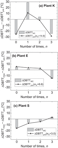
What is the essential difference between these two correction methods? It can be clearly shown that unlike the MC correction, the Bayesian correction can also evaluate the sample standard deviation ${\sigma }_X$, which is a plant-specific parameter. Some plants have high ${\sigma }_X$ values, and others have small ${\sigma }_X$ values. With this parameter, the embrittlement correlation can be improved within the framework of the probabilistic risk assessment [31,32]. This is an advantage of the Bayesian correction method, and the details will be published elsewhere.

4. Conclusion

To establish a more accurate and precise embrittlement correlation method, irradiation data were analyzed from the viewpoint of statistics, and then a new correction methodology was provided.

1. When all residual data are regarded as variables in the population, the residual data for individual plants can be considered as samples extracted from the population. To predict the $\mathrm{\Delta }\mathrm{D}\mathrm{B}\mathrm{T}\mathrm{T}$ values for a particular plant with sufficient accuracy, the sampling errors about the statistical mean should be taken into consideration.

2. To eliminate issues associated with sampling errors, an appropriate correction should be made to the JEAC 4201 calculated values. When the irradiation embrittlement of a particular plant is predicted, the conventional MC correction is still valid even from a statistical point of view, although it is not correct to use the population standard deviation as a margin.

3. As an alternative method to the MC correction, a new correction method was developed using the Bayesian estimation theory. Although this method exhibits only the same level of accuracy as that of the MC correction, it has the potential advantage of extending more useful methodology within the framework of probabilistic risk assessment.

Disclosure statement

No potential conflict of interest was reported by the authors.

Additional information

Funding

This work was supported by the Japan Society for the Promotion of Science [KAKENHI Grant Number 17J09649].

References

- Was GS. Fundamentals of radiation materials science: metals and alloys. New York: Springer; 2007.
- Odette GR, Lucas GE. Embrittlement of nuclear reactor pressure vessels. JOM: J Miner Met Mater Soc 2001 Jan;53(7):18–22.
- Phythian WJ, English CA. Microstructural evolution in reactor pressure vessel steels. J Nucl Mater. 1993 Oct;205:162–177.
- Fukuya K. Current understanding of radiation-induced degradation in light water reactor structural materials. J Nucl Sci Technol. 2013 Mar;50(3):213–254.
- Ishino S, Sekimura N, Suzuki M, et al. Present status of radiation-damage mechanism study on reactor pressure vessels based on irradiation correlation concept. J At Energy Soc Jpn. 1994 May;36:396–404. Japanese.
- Mishima Y, Ishino S, Ishikawa M, et al. PTS integrity study in Japan. Int J Pres Ves Pip. 1994;58(1):91–101.
- Ruan X, Nakasuji T, Morishita K. An investigation of the structural integrity of a reactor pressure vessel using 3D-CFD and FEM based probabilistic pressurized thermal shock analysis for optimizing maintenance strategy. J Pressure Vessel Technol. 2018 Oct;140(5):051302-051302-10.
- Tipping PG, editor. Understanding and mitigating ageing in nuclear power plants: materials and Operational Aspects of Plant Life Management (PLIM). Oxford: Woodhead publishing in energy; 2010.
- US Nuclear Regulatory Commission. Rules and regulations title 10 code of federal regulations part 50 fracture toughness requirement. Washington (DC): US Government Printing Office; 1986.
- U.S. Nuclear Regulatory Commission. regulatory guide 1.99-rev.2: radiation embrittlement to reactor pressure vessel materials. Washington (DC): US Government Printing Office; 1988.
- Eason ED, Wright JE, Odette GR. Improved embrittlement correlations for reactor pressure vessel steels. Washington DC: US Government Printing Office; 1998 Nov. (US Nuclear Regulatory Commission Report No. NUREG/CR-6551).
- Eason ED, Odette GR, Nanstad RK, et al. Physically based correlation of irradiation-induced transition temperature shifts for RPV steels. Washington (DC): US Government Printing Office; 2007. (US nuclear regulatory commission report No. ORNL-TM-2006/530).
- American Society for Testing and Materials. Standard guide for predicting radiation-induced transition temperature shift for reactor vessel materials, E706 (IIF): ASTM E900-02. West Conshohocken (PA): American Society for Testing and Materials; 2002.
- Japan Electric Association. Method of surveillance tests for structural materials of nuclear reactors: JEAC 4201-2007. Tokyo (Japan): Japan Electric Association; 2007 Dec. Japanese
- Japan Electric Association. Method of surveillance tests for structural materials of nuclear reactors: JEAC 4201-2007 [2010 addendum]. Tokyo (Japan): Japan Electric Association; 2010 Jul. Japanese
- Japan Electric Association. Method of surveillance tests for structural materials of nuclear reactors: JEAC 4201-2007 [2013 addendum]. Tokyo (Japan): Japan Electric Association; 2013 Sep. Japanese
- Soneda N, Nakashima K, Nishida K, et al. Modification of embrittlement correlation method of reactor pressure vessel steels – development of neutron irradiation embrittlement correlation of reactor pressure vessel materials of light water reactors: CRIEPI report Q06019. Tokyo (Japan): Central Research Institute of Electric Power Industry; 2007 Apr. Japanese
- Soneda N, Nakashima K, Nishida K, et al. Modification of embrittlement correlation method of reactor pressure vessel steels – calibration to the surveillance test data at high fluence –: CRIEPI report Q12007. Tokyo (Japan): Central Research Institute of Electric Power Industry; 2013 Mar. Japanese
- Soneda N, Dohi K, Nomoto A, et al. Embrittlement correlation method for the Japanese reactor pressure vessel materials: JAI102127. J ASTM Int. 2010 Feb;7(3):64–93.
- Soneda N, Dohi K, Nishida K, et al. Microstructural characterization of RPV materials irradiated to high fluences at high flux: JAI102128. J ASTM Int. 2009 Aug;6(7):129–152.
- Soneda N, Nakashima K, Nishida K, et al. High fluence surveillance data and recalibration of RPV embrittlement correlation method in Japan: PVP2013-98076. In: Barannyk O, Karri S, Oshkai P, editors. Proceedings of the ASME 2013 pressure vessels and piping conference; 2013 Jul 14–18; Paris (France). New York: American Society of Mechanical Engineers; 2013. p. 1–12.
- Nuclear Regulation Authority. Technical evaluation report on JEAC4201-2007 [2013 addendum]: method of surveillance tests for structural materials of nuclear reactors. [ updated 2015 Oct 7; cited 2019 Jul 19]:[68p.]. Available from: http://www.nsr.go.jp/data/000125554.pdf. Japanese.
- Kyushu Electric Power CO. Inc. On the integrity of reactor pressure vessels against irradiation embrittlement. [ updated 2012 Dec 21; cited 2019 Jul 19]:[10p.]. Available from: http://www.kyuden.co.jp/library/pdf/nuclear/nuclear_irradiation121221.pdf. Japanese.
- Kansai Electric Power Co. Inc. Units 1 and 2 of Takahama power station, Evaluation of degradation (neutron irradiation embrittlement of reactor vessel), supplementary explanation documents. [ updated 2016 Jun; cited 2018 Jul]. Available from: http://www.nsr.go.jp/data/000143515.pdf. Japanese.
- Shikoku Electric Power Co. Inc. On the result of surveillance tests of reactor pressure vessels in unit 1 of Ikata power station. [ updated 2013 Jul; cited 2019 Jul]:[5p.]. Available from: https://www.yonden.co.jp/press/re1307/data/pr007-01.pdf. Japanese.
- Ramachandran KM, Tsokos CP. Mathematical statistics with applications. 1st ed. Cambridge (MA): Academic Press; 2009.
- Ayyub BM, McCuen RH. Probability, statistics, and reliability for engineers and scientists. 2nd ed. Boca Raton (FL): CRC press; 2003.
- Stapleton JH. Models for probability and statistical inference: theory and applications. Hoboken (NJ): Wiley; 2007.
- Soneda N. Development of RPV embrittlement correlation method: annual report 2005 nuclear technology research laboratory. Tokyo (Japan): Central Research Institute of Electric Power Industry; 2005 Oct [ updated 2005 Oct; cited 2019 Jul]:[2p.]. Available from: https://criepi.denken.or.jp/jp/nuclear/contents/result/annual2005/5.pdf. Japanese. For more detail see also, Soneda N, English C, Server W. Use of an offset in assessing radiation embrittlement data and predictive models: PVP2006-ICPVT11-93369. In: Todd JA, Cory JF, Zamrik SY, et al., editors. Proceedings of the ASME 2006 Pressure Vessels and Piping Conference; 2006 Jul 23–27; Vancouver (Canada). New York: American Society of Mechanical Engineers; 2006. p. 351–357.
- Nuclear and Industrial Safety Agency (NISA). 5th opinion hearing on technical assessment of aging management of nuclear power plants document-2: on neutron irradiation embrittlement of reactor pressure vessel. [ updated 2012 Jan; cited 2019 Jul]:[11p.]. Available from: http://dl.ndl.go.jp/view/download/digidepo_6011694_po_5-2.pdf?contentNo=6&alternativeNo= Japanese.
- Lee JC, McCormick NJ. Risk and safety analysis of nuclear systems. Hoboken (NJ): Wiley; 2011.
- Yamamoto Y, Morishita K. Development of methodology to optimize management of failed fuels in light water reactors. J Nucl Sci Technol. 2015 May;52(5):709–716.