Loading pattern optimization for a PWR using Multi-Swarm Moth Flame Optimization Method with Predator

ABSTRACT

This paper aims to propose a new methodology for optimizing fuel loading pattern in a nuclear reactor which is important for its higher safety and economic efficiency. Previous researches have proposed various methodologies to decide better loading patterns automatically. However, the processes still require manual operations of engineers to automatically design actual loading patterns. Swarm intelligence algorithm has currently gained interest as a solution to seek the patterns. Although these methodologies generate better patterns, they sometimes struggle with getting out from local optima and fails to complete the optimization. Large and multimodal solution space sometimes captures worse solutions due to local optima. The conventional methodologies struggle with setting proper parameters to get out from local optima. This research focuses on Multi-Swarm Moth Flame Optimization with Predator (MSMFO-P), an improved Moth Flame Optimization (MFO) by applying the concepts of predator and multi-swarm, as new methodologies. The method of MSMFO-P was applied to solve a loading pattern problem and compared with the conventional optimization methods such as simulated annealing (SA), Hybrid genetic algorithm (GA), and particle swarm optimization (PSO). The results of our experimental works indicated that MSMO-P generates better loading patterns than the conventional methodologies.

KEYWORDS:

• Loading pattern
• optimization
• Moth Flame Optimization method
• PWR type reactor
• fuel assembly

1. Introduction

Optimizing fuel loading patterns is important for higher safety and economic efficiency of a nuclear reactor. In order to develop a better loading pattern, the combinational optimization problem should be solved.

Previous researches have proposed various methodologies to automatically decide better loading patterns. Main previous works until middle of the 1980s includes, the dynamic programming (1965) [1],the dual exchange search scheme (1971) [2], the direct search (1973) [3],the variational techniques (1982) [4], the backward diffusion calculation (1986) [5],the reverse depletion (1986) [6], the linear programming (1989) [7]. In the 1990s, some algorithms inspired by a natural phenomenon, such as the simulated annealing (1990) [8], were proposed. The genetic algorithm (1996) [9] is a family of these methods having a good global search capability. The hybrid GA (1997) [10], which combines GA and the local search method was proposed to increase the local search capability. After the 2000s, the swarm intelligence, which is inspired by an animal swarm movement to find feed is proposed, e.g., the particle swarm optimization (2009) [11], the artificial bee colony (2011) [12] and the ant colony(2012) [13].

However, these processes still require additional manual operations of engineers to design actual loading patterns. For example, 157 fuel assemblies are loaded in a 3-loop type PWR, thus a total number of combinations is enormous, i.e., 157! $\approx$ 10²⁵⁰. Clearly, an exhaustive search is impractical due to its huge design space and computational cost for core calculations. Automatic calculation of the loading patterns as a combination of partial optimization enables to test various scenarios in longer-term fuel management. Such extension of design capability will contribute to the safety, reliability, and economics of a reactor.

The conventional methodologies, which are introduced above, struggle with setting proper parameters to get out from local optima. The above brief review suggests that various approaches are developed and applied thanks to increasing computational resources. However, these approaches have advantages and disadvantages.

We focused on Multi-Swarm Moth Flame Optimization with Predator (MSMFO-P), an improved Moth Flame Optimization (MFO) by applying predator and multi-swarm, as new methodologies for loading pattern optimization. In this paper, MFO which is recently proposed in the computational science field is introduced and improved in this study. We focused on MFO since it has local and global search capabilities based on the swarm intelligence algorithm, which has currently gained interest as an optimization method. In addition, its search capability is expected to be improved.

The improvements applied to MFO are as follows:

• Increase capability escaping from local optima using predators.

• Improve the comprehensiveness of the search using multi-swarm.

In MSMFO-P, predators eat moths by deleting moths around the predators and randomly generate new moths to escape from local optima. The multi-swarm is also introduced by carrying out optimizations with different random seeds to cover wider design space. This paper aims to verify MSMFO-P, a new methodology for optimizing fuel loading pattern in a nuclear reactor.

The method of MSMFO-P was applied to solve a loading pattern problem and compared with the conventional optimization methods such as Simulated Annealing (SA), Hybrid GA, and Particle Swarm Optimization (PSO). The following sections are organized as follows. Section 2 describes the fundamentals of MFO and MSMFO-P. Section 3 provides calculation conditions and numerical results. Finally, section 4 summarizes concluding remarks.

2. Optimization method

2.1. Moth Flame Optimization

MFO [14] is an optimization method which is inspired by the motion of a moth. The motion of moths in the night is a fundamental idea of this method. A moth flies straight by keeping a constant angle with the light source which is far from a moth like a moon. A moth can fly wide area by this mechanism, which corresponds to the global search in the optimization method. On the other hand, a moth flies around the light and moth will not leave from the light which is close to the moth like a flame or a street lamp. A moth can fly a narrow area by this mechanism, which corresponds to the local search in the optimization method. A solution with better objective function value is set as a light source. Having sufficient distance between a moth and a light source, a moth moves widely to perform a global search. Having close distance between a moth and a light source, a moth moves around the light source. Therefore, the MFO can naturally cover both of the local search and global search depending on the distance between a moth and a light source.

MFO treats loading patterns as moths to optimize loading patterns. Light sources in the algorithm correspond to better loading patterns in the optimization process and moths approach the light sources. As an optimization progresses, the number of the light source decreases, then superior light sources gather lager number of moths. A motion of a moth naturally changes from a global search to a local search. The optimization process to apply MFO for loading pattern optimization is described as follows since MFO is used as a fundamental optimization method of the proposed method MSMFO-P. Note that the definition of the objective function is described in section 3.1.

• Step 1. Initial loading patterns are randomly generated as moths.

  • 1.1 A number of generated initial patterns (moths) are given by input. These moths compose the first generation. In the MFO, a moth has loading pattern information, e.g., k-infinity, ²³⁵U enrichment, burnable poison, and assembly burnup. First, moth_no, which is a number of initial candidate moths, and flame_no, which is the number of initial flames, are given by input. Note that moth_no ≥ flame_no. Figure 1 shows the example of the k-infinity vector of a moth and Figure 2 shows that 3 types of fuel assemblies loading positions in an octant symmetry core.

  • 1.2 One hundred times binary assembly swaps for each moth generate initial moths randomly. Note that binary swaps are carried out only within the quarter symmetry fuels and within octant symmetry fuels, i.e., no binary swap between a quarter and octant symmetry fuels is carried out.

• Step 2. Next, the objective function values of the solution candidates (moths) are evaluated using a core calculation code.

  • 2.1 The moth has loading pattern information such as as²³⁵U enrichment and so on, thus, a core calculation code can evaluate core characteristics and calculate the objective function value.

  • 2.2 The value of the objective function determines the superiority of each moth.

• Step 3. Moths and flames are sorted using the objective function value.

  Candidates of flames in the next generation are the loading patterns, which have better objective function value. Step4 ~ 5 pick flames in the next generation up from these candidates.

• Step 4. The flame_no in the next generation is calculated using Equation (1)(1) $flameno=\mathrm{r}\mathrm{o}\mathrm{u}\mathrm{n}\mathrm{d}\left(N-\mathrm{\ell }\ast \frac{N-1}{T}\right),$(1) .

  Decreasing the number of flames during the optimization process is important for the search capability. Several methods are available to decrease the number of flames. In this paper, the number of flames decreases using Equation (1)(1) $flameno=\mathrm{r}\mathrm{o}\mathrm{u}\mathrm{n}\mathrm{d}\left(N-\mathrm{\ell }\ast \frac{N-1}{T}\right),$(1) as the optimization progresses. This method has been established in the MFO [15]. Initial flame_no is given by an input. Several methods to decrease flames are compared in section 3.2.

  (1) $flameno=\mathrm{r}\mathrm{o}\mathrm{u}\mathrm{n}\mathrm{d}\left(N-\mathrm{\ell }\ast \frac{N-1}{T}\right),$(1)

  Figure 1. A fuel loading pattern and k-infinity vector.

  

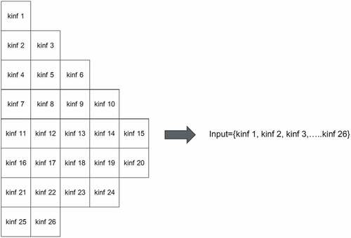
  Figure 2. Core geometry used in optimization calculations.

  

where N: maximum number of flames, $\mathrm{\ell }$: current number of generations, T: maximum number of generations

• Step 5. The candidates of flame are sorted by the objective function value.

  The moths are sorted in superior order based on the value of the objective function. Moths that have superior objective function value are saved as the flames (i.e., light sources).

• Step 6. A target flame is assigned to each moth.

  • 6.1 For example, being 100 moths and 100 flames, the different flame is assigned to each moth. Being 100 moths and 10 flames, a flame is assigned to ten moths, i.e., the target of moths 1–10 is the flame 1, that of moths 11–21 is the flame 2, and that of moths 91–100 is the flame 10.

• Step 7. Moths approach each target flame. Moving the current moth toward a flame generates a new candidate moth. Distance between the current moth and a flame determine the position of a new candidate moth. Distance is calculated by the sum of the square of the difference of assembly k-infinities. Figure 3 is an example of positions of candidate moths. The origin is the flame position and the distance between the current moth and the flame is assumed as 1.0. The dots in Figure 3 indicate examples of possible candidate position of new moth. Search naturally becomes from global search to local search depending on the distance between a flame and a moth. The global search is carried out when the distance is long while the local search is carried out for short distance. The global search tends to generate a new loading pattern that is considerably different from existing loading patterns from the viewpoint of k-infinity vector (k-infinity distribution in a core). On the other hand, the local search tends to generate a new loading pattern that has similar k-infinity vector with existing loading patterns.

  • 7.1 The distance between a moth and the assigned flame is calculated as the sum of squares of the difference of assembly k-infinities (k-infinity vector). Note that the distance is not defined as the conventional root mean square but the sum of squares of the difference of assembly k-infinities in this paper.

  • 7.2 Candidate moth position is chosen in the hypersphere whose radius is the distance calculated in 7.1, and the center of the hypersphere is the flame position. The dimension of the hypersphere is the number of assemblies. The central area of the hypersphere, which is close to the flame tends to be used as the position for a next candidate moth.

  • 7.3 A detail sampling method of the position for a next candidate moth is described as follows. The following explanation assumes a three-dimensional case for simplicity.

    • 7.3.1 The standard normal distribution generates random numbers x, y, and z to make a three-dimensional vector r = (x, y, z). The standard normal distribution is used to make isotropic sampling on direction around the origin (flame).

    • 7.3.2 The position vector from the flame is calculated as$r_{next}$ using Equation (2)(2) ${\mathit{r}}_{next}=\frac{\mathit{r}}{\left|\mathit{r}\right|}\times rand\times dist\times n,$(2) -(4(4) ${\mathit{r}}_{next}=\frac{\mathit{r}}{\left|\mathit{r}\right|}\times dist\times n,$(4) ). Choice of the equation is determined by the sensitivity study in section 3.2.

      Figure 3. Candidates of next moth position.

      
      (2) ${\mathit{r}}_{next}=\frac{\mathit{r}}{\left|\mathit{r}\right|}\times rand\times dist\times n,$(2)
      (3) ${\mathit{r}}_{next}=\frac{\mathit{r}}{\left|\mathit{r}\right|}\times ran{d}^{\frac{1}{dim}}\times dist\times n,$(3)
      (4) ${\mathit{r}}_{next}=\frac{\mathit{r}}{\left|\mathit{r}\right|}\times dist\times n,$(4)

$r_{next}$: a difference of k-infinity vector between the flame and the next candidate moth,

$\left|r\right|$：norm of $r$,

rand: uniform random number between [0,1],

dist: the distance between the current moth and the flame,

n: adjustment factor.

dim: Dimension of input

A sampling of next moth position shown in Figure 3 is carried out using Equation (2)(2) ${\mathit{r}}_{next}=\frac{\mathit{r}}{\left|\mathit{r}\right|}\times rand\times dist\times n,$(2) . The position vector (k-infinity vector) of next candidate moth is generated by adding $r_{next}$ to the position (k-infinity vector) of the current flame.

• Step 8. The generated candidate moths are composed with the k-infinity vector whose k-infinity does not correspond to actual fuel k-infinities. Therefore, the elements in a k-infinity vector of a generated moth are assigned to actual fuel assemblies as shown in Figure 4. K-infinities of the current moth in Figure 4 corresponds to the current moth position in the hyperspace and the ‘perturbation’, which is $r_{next}$, is added. These operations represent a movement of a moth. The generated moth has a k-infinity vector and ranking is assigned by the value of k-infinity. Actual fuels are loaded to specific positions using the ranking.

• Step 9. The flame_no in next generation is calculated using Equation (1)(1) $flameno=\mathrm{r}\mathrm{o}\mathrm{u}\mathrm{n}\mathrm{d}\left(N-\mathrm{\ell }\ast \frac{N-1}{T}\right),$(1) , and flame_no candidates are picked up from the top of superior candidates (including the moths and the flames). The flames in the next generation are these picked candidates. New moths in the next generation are generated using these flames.

• Step 10. Repeat Step 2 ~ 9 until the number of calculated patterns reaches to the total number of calculated loading patterns set as the termination condition.

Figure 4. Generation of candidate moth and assignment of actual fuel inventory.

2.2. Multi-Swarm Moth Flame Optimization with Predators

In this study, MFO is improved to address its weak point. First, predators have been introduced to increase the escaping capability from local optima [16]. Second, the multi-swarm concept is introduced to improve the comprehensiveness of the search [17]. The proposed method is called the multi-swarm MFO with predator (MSMFO-P). These are introduced as the improvements for PSO in the previous works.

The calculation procedures of MSMFO-P are described as follows. Steps 1 ~ 9 is operations carried out in each swarm, and Step 10 and 11 gather the results of all swarms. Figure 5 shows a flowchart. Steps 1 ~ 7 are the same as MFO.

• Step 1. Initial loading patterns are randomly generated. A number of generated initial patterns are given by input.

• Step 2. A core calculation code evaluates the objective function value.

• Step 3. Moths and flames are sorted using the objective function value.

• Step 4. The flame_no in the next generation is calculated using Equation (1)(1) $flameno=\mathrm{r}\mathrm{o}\mathrm{u}\mathrm{n}\mathrm{d}\left(N-\mathrm{\ell }\ast \frac{N-1}{T}\right),$(1) .

• Step 5. The candidates of flame are sorted by the objective function value.

• Step 6. Target flame is assigned to each moth.

• Step 7. Moths approach each target flame.

• Step 8. Moths located at the vicinity of a predator are eaten by the predator, which is introduced to eliminate moths located near the predator. Then, new moths are generated at different positions to escape a predator(a local optimum).

  • 8.1 The predator position is set at the same position as the best moth. The satiety level of predator is set to be 0, and increment of the satiety level with eaten moth is set by the input.

  • 8.2 Each predator randomly eats moth located near the predator, which is located near the predator within the parameter ViewRange in section 3.2. First, a random number [0, the maximum satiety level] is generated for each moth located near the predator. The predator does not eat a moth with the random number which is larger than the predator’s current satiety level.

  • 8.3 The capability of escaping from local optima increases but the search becomes similar to the random search when ViewRange is large. Contrary, the capability of escaping from local optima decreases when ViewRange is small. Since the setting of hypersphere radius, which is generated to choose candidate moth position, is an important factor, sensitivity analysis is carried out in section 3.2.

  • 8.4 Eating a moth increases satiety level of the predator, and the new moth is randomly born. The number of generated moths at this time is given by input.

  • 8.5 Repeating Steps 7~ Step 8.4 until the satiety level of a predator reaches a maximum, or a predator eats all target moths.

• Step 9. The generated candidate moths are composed with the k-infinity vector whose k-infinity does not correspond to actual fuel k-infinities. Therefore, actual fuel k-infinities are assigned by the same procedure with MFO.

• Step 10. Steps 2 ~ 9 are repeated while a number of calculated patterns are less than the input value, which is the same as MFO.

• Step 11. Multi-swarm optimization

  • 11.1 Steps 3 ~ 9 are carried out for each swarm using a different random seed.

  • 11.2 The best loading pattern among all swarms is the result of MSMFO-P. This process is shown in Figure 6.

Figure 5. Flowchart of MFO with predator (MFO-P).

Figure 6. Flowchart of MSMFO-P.

3. Numerical results

3.1. Calculation conditions

Figure 2 shows a core of a 3-loop PWR used in this paper. The octant symmetry is assumed with no fixed fuel assembly position except for the odd fuel assembly. The ICEBURN code, which is an in-house burnup calculation code based on diffusion theory, performs core calculations. Other calculation conditions are as follows:

• Core calculation conditions

  • Burnup calculation using burnup step of {0.0, 2.5, 5.0, 7.5, 10.0, 12.0, 12.5, 13.0, 13.5, 14.0, and 16.5} GWd/t. Fine burnup steps around the end of a cycle are adopted to accurately estimate the cycle length.

  • 1 × 1 mesh per fuel assembly using the finite-difference method

  • Two group diffusion theory

Table 1 shows the inventory of fuel assemblies used in this paper.

Table 1. Fuel inventory used for optimization calculations.

U235 Enrichment (wt%)	Burnable Poison	Burnup (GWd/t)	Number of Fuel Assemblies
4	-	34.7	1
4	-	34.7	4
4	-	34.7	4
4	-	32.2	4
4	-	32.0	8
4	-	28.9	4
4	-	27.9	8
4	-	23.8	8
4	-	23.0	4
4	-	19.5	4
4	-	19.0	8
4	-	18.9	8
4	-	18.4	8
4	-	16.8	4
4	-	16.8	4
4	-	12.6	4
4	-	12.6	4
4	-	11.3	8
4	-	10.2	8
4	-	0.0	8
4	-	0.0	8
4	-	0.0	8
4	Gd	0.0	4
4	Gd	0.0	8
4	Gd	0.0	8
4	Gd	0.0	8
Total			157

In the octant symmetry core, three different types of fuel assembly positions are considered, i.e., the odd fuel assembly at the center of the core, the 8 pair fuel assemblies at octant symmetry positions in Figure 2, and the 4 pair fuel assemblies at quarter symmetry positions in Figure 2. The followings are considered in the present study.

• The odd fuel assembly at the center of the core is fixed.

• The swap between 8 pair and 4 pair fuel assemblies is not performed

For core design, various limitations and objectives are considered to guarantee the safety and economic efficiency. In the present study, the objective function is calculated by using Equations (5(5) $objectivefunctionvalue=a\times P_{norm}+b\times C_{norm}+c\times B_{norm}$(5) )–(8(8) $B_{norm}=\left\{\begin{array}{cc}1+\frac{1}{B}\times {\left(B-B_{limit}\right)}^2& \left(B>B_{limit}\right)\\ 0& \left(B\le B_{limit}\right)\end{array}\right.$(8) ) [18]. The coefficients are set as follows through preliminary sensitivity analyses: a = 20, b = −1, c = 1, d = 0.05. Each coefficient was chosen to make the impacts of different optimization parameters similar. For example, when a large coefficient is assigned to a limitation of power peaking factor can be easily achieved but the optimization of other parameters (cycle length and maximum assembly burnup) will be difficult.

A limitation of power peaking factor P can be easily achieved but the optimization of other parameters (the cycle length C and the maximum assembly burnup B) will be difficult. The values of P, C, and B are targets in the optimization. The limitations are set as follows: $P_{limit}=1.4,B_{limit}=48$ [19]. P and B are indexes from the viewpoint of safety and C is an index from the viewpoint of economic efficiency. Therefore, the objective function includes both safety and economic aspects. Equations (5)(5) $objectivefunctionvalue=a\times P_{norm}+b\times C_{norm}+c\times B_{norm}$(5) –(8(8) $B_{norm}=\left\{\begin{array}{cc}1+\frac{1}{B}\times {\left(B-B_{limit}\right)}^2& \left(B>B_{limit}\right)\\ 0& \left(B\le B_{limit}\right)\end{array}\right.$(8) ) indicate that when the safety limitations on power peaking factor and maximum assembly burnup are achieved, loading patterns with longer cycle length is searched. Note that a negative value in the objective function shows a better loading pattern.

(5) $objectivefunctionvalue=a\times P_{norm}+b\times C_{norm}+c\times B_{norm}$(5)

(6) $P_{norm}=\left\{\begin{array}{cc}1+\frac{1}{P}\times {\left(P-P_{limit}\right)}^2& \left(P>P_{limit}\right)\\ 0& \left(P\le P_{limit}\right)\end{array}\right.$(6)

(7) $C_{norm}=d\times C$(7)

(8) $B_{norm}=\left\{\begin{array}{cc}1+\frac{1}{B}\times {\left(B-B_{limit}\right)}^2& \left(B>B_{limit}\right)\\ 0& \left(B\le B_{limit}\right)\end{array}\right.$(8)

where

P [-]: power peaking factor,

C [GWd/t]: cycle length,

B [GWd/t]: maximum assembly burnup.

For the MFO optimization, the default calculation conditions are as follows:

• Number of moths in one generation: 100

  • n in Equation (2)(2) ${\mathit{r}}_{next}=\frac{\mathit{r}}{\left|\mathit{r}\right|}\times rand\times dist\times n,$(2) –(4(4) ${\mathit{r}}_{next}=\frac{\mathit{r}}{\left|\mathit{r}\right|}\times dist\times n,$(4) ): 1

  • The initial number of flame: 100

The calculation conditions for predator are as follows:

• Initial satiety level: 0

• Increase satiety level when predator eat moth: 0.1

• Maximum satiety level: 1

• The target moth eaten by a predator: it is randomly chosen in hypersphere whose origin is the predator and the hypersphere radius, which is generated to choose candidate moth position, is given by input as the parameter ViewRange.

• Number of generated moths after a predator eats moths: number of eaten moths multiplied by an integer, which is given by input as BornCoeff shown section 3.2.

• The generation method of the reborn moth: binary fuel assembly swap is performed for 1–4 times starting from the best loading pattern. The number of swaps is randomly determined.

• Total number of calculated loading pattern during optimization: 100,000 patterns × 10 swarms = 1,000,000 patterns

3.2. Sensitivity analysis

Sensitivity analyses are carried out to choose appropriate parameters and coefficients. Table 2 shows the calculation conditions considered in the sensitivity analysis. Meaning of the parameters are summarized as follows:

• NumMoth: Number of moths in one generation in one swarm

• Fdtype: Variation of the number of flames during optimization

  • Condition 1: utilize Equation (1)(1) $flameno=\mathrm{r}\mathrm{o}\mathrm{u}\mathrm{n}\mathrm{d}\left(N-\mathrm{\ell }\ast \frac{N-1}{T}\right),$(1)

  • Condition 2: decrease by 1 at each iteration while the number of flames is larger than 1.

• FuncType: The type of sampling for next moth position in a hypersphere shown in Step 7.3.2 in section 2.1.

  • Condition 1: Dense sampling at the central region using Equation (2)(2) ${\mathit{r}}_{next}=\frac{\mathit{r}}{\left|\mathit{r}\right|}\times rand\times dist\times n,$(2) .

  • Condition 2: Uniform sampling within the hypersphere using Equation (3)(3) ${\mathit{r}}_{next}=\frac{\mathit{r}}{\left|\mathit{r}\right|}\times ran{d}^{\frac{1}{dim}}\times dist\times n,$(3) .

  • Condition 3: Uniform sampling on hypersphere surface using Equation (4)(4) ${\mathit{r}}_{next}=\frac{\mathit{r}}{\left|\mathit{r}\right|}\times dist\times n,$(4) .

• CoeffD: n in Equation (2)(2) ${\mathit{r}}_{next}=\frac{\mathit{r}}{\left|\mathit{r}\right|}\times rand\times dist\times n,$(2) –(4(4) ${\mathit{r}}_{next}=\frac{\mathit{r}}{\left|\mathit{r}\right|}\times dist\times n,$(4) )

• NumFlame: Maximum number of flames in one swarm

• EatMoth: Maximum number of eaten moths by predators at each generation

• ViewRange: View range (radius) of a predator, which is related to the position of moth eaten by a predator. A predator eats moths which are located within the ViewRange. ViewRange is not a normalized value; it directly corresponds to the radius.

• BornCoeff: Integer value multiplied to the number of eaten moths to obtain the number of reborn moths

Table 2. Calculation conditions used in the sensitivity analysis.

Case Number	NumMoth	Fdtype	FuncType	CoeffD	NumFlame	EatMoth	ViewRange	BornCoeff
0	100	1	1	1	100	10	0.5	10
1	1000	1	1	1	100	10	0.5	10
2	100	2	1	1	100	10	0.5	10
3	100	1	2	1	100	10	0.5	10
4	100	1	1	0.5	100	10	0.5	10
5	100	1	1	10	100	10	0.5	10
6	100	1	1	1	10	10	0.5	10
7	100	1	1	1	50	10	0.5	10
8	100	1	1	1	100	1	0.5	10
9	100	1	1	1	100	50	0.5	10
10	100	1	1	1	100	10	0.1	10
11	100	1	1	1	100	10	1	10
12	100	1	1	1	100	10	0.5	0.5
13	100	1	1	1	100	10	0.5	1

The optimizations are carried out ten times with different random seeds to estimate the average and the standard deviation of the objective function value of the best loading pattern. The number of swarms in MSMFO-P is chosen by an observation in the optimization process of MFO-P. In MFO-P optimization, the loading patterns significantly change during the first 10% of the whole optimization process in the present calculation condition. It means that at least 10% of the number of calculated loading patterns in MFO-P is necessary to obtain converged optimization results. Therefore, when the number of swarms is too large, the number of calculated loading pattern will be too smaller since the total number of calculated loading patterns is unchanged in MDMFO-P. Therefore, the number of swarms are decided as 10. Figure 7 shows the average and the standard deviation of the objective function.

Figure 7. Result of sensitivity analysis of MSMFO-P.

The range of average ± standard deviation (the standard deviation of 10 results) overlaps. The following observations are obtained from the results:

• Optimization parameters have small sensitivity for optimization results since multi-swarm is introduced. In the process of multi-swarm, the optimization result is chosen from the best solutions obtained by the several independent optimizations in swarms. Therefore, variation in optimization results becomes smaller. Note that the statistical test indicates MSMFO-P is better than MSMFO thus the introduction of predators is still effective using MS.

• Small sensitivity of optimization parameters is a superior point of the proposed method since small sensitivity implies the robustness of the optimization method.

• In the following section, the parameters of case number 0 in Table 2 are used for the optimization calculations by MSMFO-P since no significant difference of optimization performance is observed among the calculation cases and the case number 0 is the base case of perturbation in the sensitivity analysis.

3.3. Optimization parameters of the conventional methods

Table 3 shows the optimization parameters of the conventional methods (SA [8], Hybrid GA [10], PSO [11]). The PSO is carried out using Equations (9)(9) $v_{ij}\left(t+1\right)=w^t{v}_{ij}\left(t\right)+c_1{r}_1\left(t\right)\left(p_{ij}\left(t\right)-x_{ij}\left(t\right)\right)+c_2{r}_2\left(t\right)\left(p_{gj}\left(t\right)-x_{ij}\left(t\right)\right)$(9) –(11(11) $w^t=\frac{w_{max}-w_{min}}{t_{max}}t$(11) ). The parameters in PSO are appropriately determined by sensitivity analysis.

(9) $v_{ij}\left(t+1\right)=w^t{v}_{ij}\left(t\right)+c_1{r}_1\left(t\right)\left(p_{ij}\left(t\right)-x_{ij}\left(t\right)\right)+c_2{r}_2\left(t\right)\left(p_{gj}\left(t\right)-x_{ij}\left(t\right)\right)$(9)

(10) $x_{ij}\left(t+1\right)=x_{ij}\left(t\right)+v_{ij}\left(t+1\right)$(10)

Table 3. Calculation conditions of the conventional optimization methods.

SA	Initial temperature	1
	Cooling rate	0.99029/1000	calculations
	Number of assemblies in one swap	1–3
	Number of assembly swap	1–3
Hybrid GA	Number of populations	60
	Number of survived candidates after selection	50
	Number of binary swaps for random mutaion	5
	Tournament size	5
	Probability of random mutation	0.1
	Probability of crossover	0.99
PSO	Number of particles in one generation	500
	c1 in Equation (9)(9) $v_{ij}\left(t+1\right)=w^t{v}_{ij}\left(t\right)+c_1{r}_1\left(t\right)\left(p_{ij}\left(t\right)-x_{ij}\left(t\right)\right)+c_2{r}_2\left(t\right)\left(p_{gj}\left(t\right)-x_{ij}\left(t\right)\right)$(9)	2.4
	c2 in Equation (9)(9) $v_{ij}\left(t+1\right)=w^t{v}_{ij}\left(t\right)+c_1{r}_1\left(t\right)\left(p_{ij}\left(t\right)-x_{ij}\left(t\right)\right)+c_2{r}_2\left(t\right)\left(p_{gj}\left(t\right)-x_{ij}\left(t\right)\right)$(9)	2.4
	w_max in Equation (11)(11) $w^t=\frac{w_{max}-w_{min}}{t_{max}}t$(11)	0.9
	w_min in Equation (11)(11) $w^t=\frac{w_{max}-w_{min}}{t_{max}}t$(11)	0.4

The weight is updated by:

(11) $w^t=\frac{w_{max}-w_{min}}{t_{max}}t$(11)

where

i: the particle number,

j: the position number of input vector elements,

$t$: the current number of iterations,

$t_{max}$: the maximum number of iterations,

$w^t$: the weight at iteration t,

$v_{ij}\left(t\right)$: velocity,

$r_1\left(t\right),r_2\left(t\right)$: random number of [0, 1],

$x_{ij}\left(t\right)$: current position,

$x_{ij}\left(t+1\right)$: candidate position at iteration $t+1$,

$p_{ij}\left(t\right)$: the best solution found by particle i,

$p_{gj}\left(t\right)$: the global best solution,

$c_1$: the influence of the best solution found by individual particle,

$c_2$ the influence of the global optimal solution found by all particles,

The parameters $w_{max}$, $w_{min}$, $c_1$, and $c_2$ are set by input and are summarized in Table 3.

3.4. Results and discussions

3.4.1. Results

The optimization results of the proposed method are shown in Table 4, and the results of conventional methods are shown in Tables 5–7. The optimization parameters used in these optimizations are chosen as described in section 3.3. In an optimization run, 100,000 core calculations are carried out for each optimization method, MSMFO-P, SA, HybridGA, and PSO.

Table 4. Optimization results of MSMFO-P.

Initial random seed	Objective function value [-]	Power peaking factor [-]	Cycle length [Gwd/t]	Assembly mximum burnup [Gwd/t]
1	−0.9888	1.3954	19.7769	47.9607
2	−0.9884	1.3988	19.7673	47.1154
3	−1.0038	1.3881	20.0765	47.5023
4	−0.9921	1.3981	19.8427	47.6035
5	−0.9998	1.3976	19.9952	47.1899
6	−0.9834	1.3944	19.6671	47.9761
7	−1.0041	1.3993	20.0819	47.6675
8	−0.9873	1.3974	19.7462	44.8057
9	−0.9927	1.3909	19.8532	47.4170
10	−1.0053	1.3889	20.1061	47.0931
Average (within limits)	−0.9946	1.3949	19.8913	47.2331
Standard deviation (within limits)	0.0080	0.0042	0.1603	0.9093

Table 5. Optimization results of SA.

Initial random seed	Objective function value [-]	Power peaking factor [-]	Cycle length [Gwd/t]	Assembly maximum burnup [Gwd/t]
1	−0.9709	1.3980	19.4185	45.8646
2	−0.9731	1.3876	19.4614	47.6073
3	−0.9555	1.3832	19.1109	47.6174
4	−0.9631	1.3803	19.2613	47.4817
5	−0.9661	1.3978	19.3221	47.3424
6	−0.9708	1.3932	19.4156	47.3677
7	−0.9581	1.3870	19.1625	46.3525
8	−0.9583	1.3804	19.1663	46.2128
9	−0.9544	1.3906	19.0888	47.9333
10	−0.9553	1.3960	19.1054	46.9831
Average (within limits)	−0.9626	1.3894	19.2513	47.0763
Standard deviation (within limits)	0.0072	0.0068	0.1440	0.6973

Table 6. Optimization results of Hybrid GA.

Initial random seed	Objective function value [-]	Power peaking factor [-]	Cycle length [Gwd/t]	Assembly maximum burnup [Gwd/t]
1	−0.9553	1.3959	19.1064	47.2429
2	−0.9871	1.39777	19.7429	45.6215
3	−0.9343	1.39846	18.6858	45.3398
4	−0.9601	1.39242	19.2019	47.1136
5	−0.9549	1.39954	19.0987	43.4144
6	−0.9603	1.39387	19.2069	46.8826
7	−0.9606	1.38456	19.2122	47.8374
8	−0.9585	1.3996	19.1704	46.6201
9	−0.9754	1.39984	19.5072	45.7462
10	−0.9832	1.39638	19.6642	45.4915
Average (within limits)	−0.9630	1.3958	19.2597	46.1310
Standard deviation (within limits)	0.0154	0.0047	0.3080	1.2798

Table 7. Optimization results of PSO.

Initial random seed	Objective function value [-]	Power peaking factor [-]	Cycle length [Gwd/t]	Assembly maximum burnup [Gwd/t]
1	−0.9534	1.3926	19.0684	47.1146
2	−0.9290	1.3969	18.5804	46.9788
3	−0.9243	1.3995	18.4853	47.1263
4	19.0132	1.4071	19.7507	47.8684
5	−0.9602	1.3965	19.2050	47.8062
6	−0.9593	1.3788	19.1855	47.7289
7	−0.9774	1.3998	19.5486	44.8491
8	−0.9599	1.3998	19.1975	47.6917
9	−0.9556	1.3939	19.1121	45.6608
10	−0.9218	1.3904	18.4361	46.2739
Average (within limits)	−0.9490	1.3942	18.9799	46.8034
Standard deviation (within limits)	0.0193	0.0067	0.3855	1.0179

Table 4 to Table 7 include the result whose objective function value is positive. The positive objective function value means that the limitations on power peaking factor and/or maximum assembly burnup are violated such as $\mathrm{P}>{\mathrm{P}}_{\mathrm{l}\mathrm{i}\mathrm{m}\mathrm{i}\mathrm{t}}$ and/or $\mathrm{B}>{\mathrm{B}}_{\mathrm{l}\mathrm{i}\mathrm{m}\mathrm{i}\mathrm{t}}$ in Equation (6)(6) $P_{norm}=\left\{\begin{array}{cc}1+\frac{1}{P}\times {\left(P-P_{limit}\right)}^2& \left(P>P_{limit}\right)\\ 0& \left(P\le P_{limit}\right)\end{array}\right.$(6) and (8(8) $B_{norm}=\left\{\begin{array}{cc}1+\frac{1}{B}\times {\left(B-B_{limit}\right)}^2& \left(B>B_{limit}\right)\\ 0& \left(B\le B_{limit}\right)\end{array}\right.$(8) ). The average and standard deviation of objective function values excluding the positive value are summarized in Figure 8 since a loading pattern with positive objective function value violates the safety limitations thus is not feasible. Excluding positive value is because a loading pattern which does not satisfy safety limits is not considered in the core design. Figure 8 suggests that the MSMFO-P optimization generates better results than those generated by the conventional methods.

Figure 8. Comparison of objective function values satisfying limits.

Loading patterns generated by the proposed and conventional methods are shown in Figure 9. The value of k-infinity is also shown in Figure 9. In Figure 9, the fresh fuels are located not only in the core peripheral region but also the inner core region and burned fuels having low k-infinity are located in the core peripheral region. This type of loading pattern is a low leakage loading pattern (L3P). The cycle length of L3P is longer due to lower leakage of neutron from a core [20].

Figure 9. Example of generated loading patterns by (a) MSMFO-P, (b) SA, (c) Hybrid GA, (d) PSO. Value in the assembly indicates k-infinity.

When the limitations of the power peaking factor and assembly maximum burnup are satisfied, the objective function value depends on only the cycle length. In this paper, L3P is defined as that number of burned fuels loaded core peripheral region is larger than that of fresh fuels. Table 8 shows the number of generated L3P in 10 trials, which is counted when L3P is obtained as the final result. All loading patterns generated by MSMFO-P are L3P.

Table 8. Number of L3P loading patterns in which fresh fuel assemblies without Gd are loaded core inboard in 10 trials.

MSMFO-P	SA	HybridGA	PSO
10	5	4	5

3.4.2. Discussions

In order to make a discussion on optimization performances of MSMFO-P and the conventional methods, the L3P index is newly introduced that represents the magnitude of neutron leakage from a core. The L3P index is defined by the weighted sum of assembly burnups in the core periphery. The weight to calculate the L3P index is a number of faces adjacent to baffle, e.g., a fuel assembly adjacent to baffle through two faces has a weight of 2.0. The L3P index increases for a low leakage core in which highly burned fuel assemblies are loaded at the core periphery region.

At first, in order to compare the optimization performances of MFO, MFO-P, MSMFO, and MSMFO-P, the maximum values of L3P index in the last generation of these methods are shown in Table 9. Note that MSO-P and MSMFO represent MFO coupled with predator and MFO coupled with multi-swarm, respectively.

Table 9. Average and standard deviations of the L3P indexes in the last generation of MFO, MFO-P, MSMFO, and MSMFO-P.

	MFO	MFO-P	MSMFO	MSMFO-P
Average	112.62	145.06	161.59	182.33
Standard deviation	34.93	36.12	22.47	20.11
Relative standard deviation	0.31	0.25	0.14	0.11

The k-s test [21] shows statistically significant differences in the L3P index among methods. Namely, two improvements, i.e., predator (P) and multi-swarm (MS) for MFO surely improve the optimization performance. The objective function values are shown in Table 10. The statistical test of results in Table 10 shows that the introduction of the predator and the multi-swarm increases optimization performance.

Table 10. Average and standard deviations of the objective function of MFO, MFO-P, MSMFO, and MSMFO-P.

	MFO	MFO-P	MSMFO	MSMFO-P
Average	−0.9608	−0.9773	−0.9782	−0.9917
Standard deviation	0.0169	0.0152	0.0112	0.0101
Relative standard deviation	0.0176	0.0156	0.0115	0.0102

Introduction of predators increases the local search capability by generating a better solution through small perturbations. Approximately 90% of the best solutions obtained in each generation are generated by the local search regarding to predators. Comparing the L3P indexes for MFO and MSMFO, the introduction of MS significantly reduces the standard deviation of the L3P index. Since MS performs independent multiple optimizations starting from different initial loading patterns, global search capability increases. The optimization results are less trapped in the local optima thus the standard deviation of the L3P index reduces. Figure 8 indicates that the standard deviation of the objective function values is larger for Hybrid-GA and PSO, indicating that these methods tend to be trapped into local optima. Applying MS to the conventional methods (SA, Hybrid-GA, and PSO), performance improves in Hybrid-GA and PSO. This result also supports the discussion on MS capability of escaping from local optima.

Next, the difference of optimization performance among the present and the conventional methods are discussed. Figure 10 shows a comparison of the average L3P index during100 optimization trials using different random seeds. The horizontal axis is normalized so that the largest generation corresponds to 1.0.

Figure 10. Averages of maximum L3P index of each method.

In the beginning of optimization, the L3P indexes are large and similar among different methods since loading patterns are randomly generated. Then the L3P indexes decrease in order to satisfy the limitations of power peaking factor and maximum burnup. Note that, an L3P core with a higher L3P index tends to have a higher power peaking factor since assembly power at the core peripheral region is low. Once the L3P indexes decrease then they begin to increase by the end of optimization. The final result depends on the degree of reduction of the L3P index at the early optimization stage and their recovery at the latter stage. In MSMFO-P, peripheral fuel assembly positions are changed in approximately 10% of newly generated loading patterns while the probability is 30–40% in the conventional methods. Low probability of changing peripheral fuel assemblies in MSMFO-P contributes to suppress reduction of the L3P index at the early optimization stage and thus contributes to its higher performance. For the reasons described above, loading patterns having a higher L3P index tend to survive in the early stage of optimization in MSMFO-P and they push up its optimization performance.

4. Conclusions

Optimization of fuel loading patterns is important for higher safety and economic efficiency of a nuclear reactor. Previous researches have proposed various methodologies to automatically decide better loading patterns. However, these methodologies have their advantages and disadvantages.

Recently, swarm intelligence has been applied for the loading pattern optimization problems. In this research, we focused on Multi-Swarm Moth Flame Optimization with Predator (MSMFO-P), which is an improved Moth Flame Optimization (MFO) by applying predator and multi-swarm as new methodologies. However, MFO has difficulty to escape from local optima. MSMFO-P generates better loading pattern than the conventional methodologies (SA, hybrid GA, and PSO), and sensitivity analysis shows that MSMFO-P has small sensitivity on optimization parameters because of the multi-swarm nature. The reason for the better optimization performance of MSMFO-P is discussed by comparing the optimization performances of MFO, MFO-P, MSMFO, MSMFO-P, and the conventional methods. The choice of optimization parameters is not very difficult in MSMFO-P, and it would provide a robust result on actual applications. Setting parameters of predators and the number of swarms are future works to further improve the optimization performance.

Disclosure statement

No potential conflict of interest was reported by the authors.

References

- Wall I, Fenech H. The application of dynamic programming to fuel management optimization. Nucl Sci Eng. 1965;22:285–297.
- Naft NB, Sesonske A. Pressurized water reactor optimal fuel management. Nucl Technol. 1971;14:123–132.
- Stout BR Optimization of in-core nuclear fuel management in a pressurized water reactor [dissertation]. Corvallis(OR): Oregon State University at Oregon; 1973.
- Terney BW, Williamson AE Jr. The design of reload cores using optimal control theory. Nucl Sci Eng. 1982;82:260–288.
- Chao YA, Hu CW, Suo CA. A theory of fuel management via backward diffusion calculation. Nucl Sci Eng. 1986;93:78–87.
- Downar. JT, Kim. JY. A reverse depletion method for pressurized water reactor core reload design. Nucl Sci Eng. 1986;93:78–87.
- Stillman AJ, Chao AY, Downar JT. The Optimum fuel and power distribution for a pressurized water reactor burnup cycle. Nucl Sci Eng. 1989;103:321–333.
- Parks TG. An intelligent stochastic optimization routine for nuclear fuel cycle design, nuclear technology. Nucl Technol. 1990;89:223–246.
- Parks TG. Multiobjective pressurized water reactor reload core design by nondominated genetic algorithm search. Nucl Sci Eng. 1996;124:178–187.
- Yamamoto A Study on advanced in-core fuel management for pressurized water reactors using loading pattern optimization methods [dissertation]. Kyoto: Kyoto University at Kyoto; 1998.
- Meneses MAA. Particle swarm optimization applied to the nuclear reload problem of a pressurized water reactor. Prog Nucl Energy. 2009;51:319–326.
- Safarzadeh A, Zolfaghari A, Norouzi A, et al. Loading pattern optimization of PWR reactors using artificial bee colony. Ann Nucl Energy. 2011;38:2218–2226.
- Lin C, Lin FB. Automatic pressurized water reactor loading pattern design using ant colony algorithms. Ann Nucl Energy. 2012;43:91–98.
- Mirjalili S. Moth-flame optimization algorithm: a novel nature-inspired heuristic paradigm. Knowledge-Based Syst. 2015;89:228–229.
- Sayed IG, Hassanien EA. A hybrid SA-MFO algorithm for function optimization and engineering design problems. Complex Intell Syst. 2018;4:195–212.
- Inukai N, Inoue T, Uwate Y, et al. Investigation of particle swarm optimization with predator. Tokyo: the institute of electronics, information and communication engineers; 2013. (Technical Report of IEICE; Report No. 113 p. 109–112).
- Xia X, Gui L, Zhan Z. A multi-swarm particle swarm optimization algorithm based on dynamical topology and purposeful detecting. Appl Soft Comput. 2018;67:126–140.
- Park KT, Lee CH, Foo KH, et al. Loading pattern optimization by multi-objective simulated annealing with screening technique. In: Proceedings of PHYSOR-2006;2006 Sep 10–14; Vancouver, BC, Canada. Vancouver (BC): The Canadian Nuclear Society; 2006.
- Genshirosekkei OY. [Design of reacotor]. Tokyo: Ohmsha; 2010. Japanese. p. 113,156.
- Chang CY, Sesonske A. Optimization and analysis of low-leakage core management for pressurized water reactors. Nucl Technol. 1984;65:292–304.
- The R project for statistical computing [Internet]. Vienna(Austria): R Foundation for Statistical Computing; cited 2019 June 14]. Available from . https://www.R-project.org/