Modeling of gap conductance for LWR fuel rods applied in the BISON code

ABSTRACT

A new gap conductance model is proposed in this study as a combination of Toptan’s model and the Ross-Stoute model. A variance-based sensitivity analysis is performed to understand how simulation results depend on all input parameters of the proposed model. Additionally, new modeling options (e.g. fill gas thermal conductivity, temperature jump distance, thermal accommodation coefficient, etc.) are added into the nuclear fuel performance code, BISON. The need for further investigation of the gap heat transfer between fuel and cladding in BISON motivated this study to evaluate its impact on the code’s predictions. New gap conductance modeling is proposed. A series of integral-effects validation tests is performed: (1) to demonstrate the impact of the proposed model on the code’s fuel temperature predictions at the beginning of life and through the reactor’s life; (2) to ensure that the proposed model is capable of accurately modeling gap heat transfer characteristics in real-world problems; and (3) to investigate the impact of the estimation of fission gas release on the fuel temperature predictions with the proposed model. The results indicate that the proposed gap conductance model improves BISON’s predictions.

KEYWORDS:

• BISON
• fuel performance
• gap conductance
• gap heat transfer
• validation
• LWR

1. Introduction

The model conventionally used to compute heat transfer across the fuel-cladding gap in light water nuclear reactors is a modified version of the Ross-Stoute model. The original model [1] was modified to include gap distance in the formulation to account for the gap evolution in nuclear fuel applications [2–6]. This introduced additional uncertainties because the model parameters were not adjusted after the modification. This conventional model was optimized for uranium dioxide–Zircaloy interfaces using experimental data at high pressure for single – and multi-component gases by Toptan et al. [7]. However, the model applies to light contact between fuel pellet and cladding. In this study, a gap conductance model is proposed which is also valid for large loads on the contact surfaces (large contact pressures). Later, a series of integral-effects validation tests is performed to demonstrate the code’s predictions with the improved gap heat transfer modeling at the beginning of life (BOL) and through reactor life using a finite-element-based nuclear fuel performance code, BISON [2]. BISON is a state-of-the-art fuel performance code for modeling nuclear thermomechanical behavior and is applicable to a variety of fuel types. The code has been developed by Idaho National Laboratory (INL) and solves the fully coupled equations of thermomechanics and species diffusion in multi-dimensions. The code is based on the Multiphysics Object-Oriented Simulation Environment (MOOSE) framework, a high-performance, open-source finite element toolkit developed at INL. Williamson et al. [8] indicated the need to further investigate the gap heat transfer between fuel and cladding in BISON. This study aims to evaluate its impact on BISON’s predictions with enhanced gap conductance modeling. Note that only the thermal aspects of the gap are considered in this study.

A background on the gap conductance modeling is provided in Section 2. A variance-based sensitivity analysis is performed to investigate the influential parameters of the gap conductance model in Section 3. The BISON predictions are validated against the experimental data by performing a series of validation tests to ensure that the code is capable of accurately modeling real-world problems. The results and discussion of the validation are given in Section 4. Concluding remarks and future work are discussed in Section 5.

2. Thermal model across the fuel–cladding gap

Total conductance across the gap is computed as three summed heat paths: fill gas conductance ($h_g$), direct thermal radiation ($h_r$), and solid contact conductance ($h_s$):

(1) $h_{gap}=h_g+h_s+h_r.$(1)

BISON models the gap conductance using a modified version of the Ross–Stoute model [1]. Conductance due to the thermal radiation is also included and is taken from Bird et al. [9] with a unity ratio of the areas.

(2) $h_{gap}=\frac{{\lambda }_g}{d+{\theta }_1({\xi }_1+{\xi }_2)+(g_1+g_2)}+\frac{{\theta }_2\mathrm{\Lambda }}{\sqrt{{\xi }_1+{\xi }_2}}\left(\frac{W}{H}\right),$(2)

where ${\lambda }_g$ is gas thermal conductivity, $d$ is gap distance, $\xi$ is surface roughness which is defined as a one-dimensional parameter to represent the mean deviation of surface irregularities, $g$ is temperature jump distance, $\mathrm{\Lambda }=\left(\frac{2{\lambda }_1{\lambda }_2}{{\lambda }_1+{\lambda }_2}\right)$ is the harmonic mean of thermal conductivities of the surrounding solids (1 for fuel; 2 for clad in this study), $W$ is load on the contact interface (or contact pressure), $H$ is Meyer’s hardness of the softer material, ${\theta }_1$ (1.5 in default) is the roughness coefficient, and ${\theta }_2$ ($10.0/\sqrt{0.8}$ in default) is the contact coefficient.

The original Ross-Stoute model [1] is given by

(3) $\begin{array}{cc}{h}_{gap}& =\frac{{\lambda }_g}{{\theta }_1({\xi }_1+{\xi }_2)+(g_1+g_2)}+\frac{{\theta }_2\mathrm{\Lambda }}{\sqrt[4]{{\xi }_1^2+{\xi }_2^2}}\left(\frac{W}{H}\right),\\ \theta & =\{{\theta }_1,{\theta }_2\}=\left\{1.2,\frac{10.0}{\sqrt[4]{0.5}}\right\},\end{array}$(3)

which underlies the assumption of plastically deformed surface irregularities at contact. The load was ranged from approximately 5.0 to 54.0 MPa in their experiment.

BISON’s model was modified to include gap distance $d$ in Equation (3)(3) $\begin{array}{cc}{h}_{gap}& =\frac{{\lambda }_g}{{\theta }_1({\xi }_1+{\xi }_2)+(g_1+g_2)}+\frac{{\theta }_2\mathrm{\Lambda }}{\sqrt[4]{{\xi }_1^2+{\xi }_2^2}}\left(\frac{W}{H}\right),\\ \theta & =\{{\theta }_1,{\theta }_2\}=\left\{1.2,\frac{10.0}{\sqrt[4]{0.5}}\right\},\end{array}$(3) , which introduced additional uncertainty because the model parameters were not adjusted after the modification. To understand sources of the uncertainties in the gap conductance model due to the inclusion of the gap thickness, Toptan et al. [7,10] calibrated the following model

(4) $\begin{array}{rl}& h_{gap}=\frac{{\lambda }_g}{d+{\theta }_1({\xi }_1+{\xi }_2)+(g_1+g_2)}+\frac{{\theta }_2\mathrm{\Lambda }}{\sqrt{{\xi }_1^2+{\xi }_2^2}}\left(\frac{W}{H}\right),\\ & \theta =\{{\theta }_1,{\theta }_2\}=\{0.605,14.522\},\end{array}$(4)

using the available literature data for uranium dioxide and Zircaloy-4 interfaces by Garnier and Begej [11] at temperatures from 283 to 673 K and fill gas pressures from 0.1 to 7 MPa for light contact (i.e., the load was 1300 N/m${ }^2$). The model was calibrated with helium, argon, and their binary mixture. The data include the gap thickness information. As mentioned in their paper, additional data are necessary for more representative gas compositions in a nuclear fuel setting. The results can be repeated with the additional experimental data with the established procedure in [7].

The advantages and disadvantages of the aforementioned models are listed below:

• Equation (3)(3) $\begin{array}{cc}{h}_{gap}& =\frac{{\lambda }_g}{{\theta }_1({\xi }_1+{\xi }_2)+(g_1+g_2)}+\frac{{\theta }_2\mathrm{\Lambda }}{\sqrt[4]{{\xi }_1^2+{\xi }_2^2}}\left(\frac{W}{H}\right),\\ \theta & =\{{\theta }_1,{\theta }_2\}=\left\{1.2,\frac{10.0}{\sqrt[4]{0.5}}\right\},\end{array}$(3) does not include the gap thickness; however, Ross and Stoute have data in a vacuum where the contact coefficient, ${\theta }_2$ was estimated (i.e., independent of the roughness coefficient, ${\theta }_1$).

• Equation (4)(4) $\begin{array}{rl}& h_{gap}=\frac{{\lambda }_g}{d+{\theta }_1({\xi }_1+{\xi }_2)+(g_1+g_2)}+\frac{{\theta }_2\mathrm{\Lambda }}{\sqrt{{\xi }_1^2+{\xi }_2^2}}\left(\frac{W}{H}\right),\\ & \theta =\{{\theta }_1,{\theta }_2\}=\{0.605,14.522\},\end{array}$(4) applies for light contact as the applied load in the data was 1300 N/m${ }^2$; however, the roughness coefficient, ${\theta }_1$ can simply be assumed independent of the contact effects because the Meyer’s hardness of the cladding (i.e., the softer material) is on the order of approximately 1 $\times {10}^9$Pa; therefore, the load-to-hardness, $(W/H)$ was on the order of 1 $\times {10}^{-6}$.

Here, the following model is postulated as a combination of Toptan’s model and the Ross-Stoute model:

(5) $\begin{array}{cc}{h}_{gap}& =\frac{{\lambda }_g}{d+0.605({\xi }_1+{\xi }_2)+(g_1+g_2)}+\frac{10\mathrm{\Lambda }}{\sqrt[4]{0.5({\xi }_1^2+{\xi }_2^2)}}\left(\frac{W}{H}\right),\\ \theta & =\{{\theta }_1,{\theta }_2\}=\left\{0.605,\frac{10.0}{\sqrt[4]{0.5}}\right\}\end{array}$(5)

To overcome the shortcoming of other models and to be representative at high gas pressures and larger contact pressures in nuclear applications: (1) the gap thickness is included in the fill gas conductance term and ${\theta }_1$ is from [7] using the Garnier–Begej data at high gas pressures and (2) the contact effects at larger loads are included, using Ross-Stoute formulation. The proposed model will be validated in this paper. The default and newly added models in BISON are tabulated in Table 1 for the fill gas thermal conductivity, the thermal accommodation coefficient, temperature jump distance, and Meyer’s hardness of the softer material (e.g., the cladding). An overview of the theoretical considerations and the underlying assumptions of gap conductance modeling, as well as the traditional modeling approaches in many nuclear fuel performance codes, is provided in [12].

Table 1. Brief summary of the models that are available in BISON.

Default	New feature
Fill gas thermal conductivity models
Based on MATPRO-11 [13]	Pressure-effects are included to the code [20].
$\lambda ($W/m-K$)=a{T}^b$	$\lambda ($W/m-K$)={\lambda }^0(T)+{\lambda }_c^{\star }{\mathrm{\Psi }}_k\left(\frac{\rho }{{\rho }_c}\right)$
where	where
$T=$ temperature (K)	$\lambda =$ thermal conductivity of pure dilute gas (W/m-K)
$a,b=$ empirical coefficients vary for each gas	${\lambda }_c^{\star }=$ pseudo-critical thermal conductivity (W/m-K)
	${\mathrm{\Psi }}_k\left(\rho /{\rho }_c\right)$= the excessive thermal conductivity
	$\rho$= gas density (see Appendix A)
Temperature jump distance models
Kennard’s model based on a review by [14]	Kennard’s model based on a review by [12]
$g($cm$)=2878\left(\frac{2-\alpha }{\alpha }\right)\left(\frac{\lambda \sqrt{T}}{P}\right){\left(\frac{1}{{\sum }_{i=1}^n{f}_i/M_i}\right)}^{1/2}$	$g$(m)$=\frac{\sqrt{8\pi }}{(1+\gamma )\nu }\frac{\lambda }{P{\mathrm{\Lambda }}_{12}}\sqrt{\frac{T}{R_{g}M}}$
where	where
$T=$ temperature (K)	$T=$ temperature (K)
$P=$ pressure (dyne/cm${ }^2$)	$P=$ pressure (Pa)
$\lambda =$ fill gas thermal conductivity (cal/sec-cm-${ }^{\circ }$C)	$\lambda =$ fill gas thermal conductivity (W/m-K)
$M=$ molecular weight of gas constituent (g/mole)	$M=$ molecular weight of gas constituent (g/mole)
$f=$ mole fraction	$R_g=$ ideal gas constant (8.314 J/mol-K)
$\alpha =$ thermal accommodation coefficient	$\alpha =$ thermal accommodation coefficient
	$\frac{\sqrt{8\pi /R_g}}{(1+\gamma )\nu }=\left\{\begin{array}{cc}0.2173& \mathrm{f}\mathrm{o}\mathrm{r}\mathrm{t}\mathrm{h}\mathrm{e}\mathrm{m}\mathrm{o}\mathrm{n}\mathrm{a}\mathrm{t}\mathrm{o}\mathrm{m}\mathrm{i}\mathrm{c}\mathrm{g}\mathrm{a}\mathrm{s}\mathrm{e}\mathrm{s},\\ 0.1149& \mathrm{f}\mathrm{o}\mathrm{r}\mathrm{t}\mathrm{h}\mathrm{e}\mathrm{d}\mathrm{i}\mathrm{a}\mathrm{t}\mathrm{o}\mathrm{m}\mathrm{i}\mathrm{c}\mathrm{g}\mathrm{a}\mathrm{s}\mathrm{e}\mathrm{s},\\ 0.1242& \mathrm{f}\mathrm{o}\mathrm{r}\mathrm{t}\mathrm{h}\mathrm{e}\mathrm{p}\mathrm{o}\mathrm{l}\mathrm{y}\mathrm{a}\mathrm{t}\mathrm{o}\mathrm{m}\mathrm{i}\mathrm{c}\mathrm{g}\mathrm{a}\mathrm{s}\mathrm{e}\mathrm{s}.\end{array}\right.$
	${\mathrm{\Lambda }}_{12}=\left\{\begin{array}{cc}\frac{\alpha }{2-\alpha }& \mathrm{p}\mathrm{l}\mathrm{a}\mathrm{n}\mathrm{e},\\ \frac{\alpha }{1+(1-\alpha )r_1/r_2}& \mathrm{c}\mathrm{y}\mathrm{l}\mathrm{i}\mathrm{n}\mathrm{d}\mathrm{e}\mathrm{r},\\ \frac{\alpha }{1+(1-\alpha )(r_1/r_2{)}^2}& \mathrm{s}\mathrm{p}\mathrm{h}\mathrm{e}\mathrm{r}\mathrm{e}.\end{array}\right.$
Thermal accommodation coefficient models
based on a review by [14]	Toptan’s model [12]
$\alpha ={\alpha }_{He}+\frac{({\alpha }_{Xe}-{\alpha }_{He})(M_{mix}-M_{He})}{(M_{Xe}-M_{He})}$	$\alpha =1-\left(1-{\alpha }_{\mathrm{\infty }}tanh\left[\frac{\sqrt{m_{i}T}}{{\alpha }_{\mathrm{\infty }}}{\theta }_1\right]\right)exp\left(-\frac{{\theta }_2}{T}\right)$
where	where
${\alpha }_{He}=0.423-2.3\times {10}^{-4}T$	$T=$ temperature (K)
${\alpha }_{Xe}=0.749-2.5\times {10}^{-4}T$	${\alpha }_{\mathrm{\infty }}=2.4\mu /(1+\mu {)}^2$
$T=$ temperature (${ }^{\circ }$C)	$\mu =(M_i/M_s)$, the ratio of molecular weights
	$\theta =\{{\theta }_1,{\theta }_2\}$= the coefficient matrix
Meyer’s hardness models
an average value by [15]	MATPRO model [13]
$H$(N/m${ }^2)=$0.68 $\times {10}^9$	$H$(N/m${ }^2)=exp(26.034-2.6394\times {10}^{-2}T+4.35\times {10}^{-5}$$T^2+2.5621\times {10}^{-8}{T}^3)$
	where
	$T=$ temperature (K)

3. Sensitivity analysis

Sensitivity analysis (SA) is a process used to understand how simulation results depend on all input parameters, assumptions, or mathematical models as well as to inform the user about the most important factors in uncertain results [16]. In this study, Sobol’ method (Appendix B) is utilized to identify the most influential parameter out of the selected input parameters ($d$, ${\xi }_1$, ${\xi }_2$, $T$, $P$, ${\theta }_1$, ${\theta }_2$, and the load-to-hardness ratio $(W/H)$) in Equation (5)(5) $\begin{array}{cc}{h}_{gap}& =\frac{{\lambda }_g}{d+0.605({\xi }_1+{\xi }_2)+(g_1+g_2)}+\frac{10\mathrm{\Lambda }}{\sqrt[4]{0.5({\xi }_1^2+{\xi }_2^2)}}\left(\frac{W}{H}\right),\\ \theta & =\{{\theta }_1,{\theta }_2\}=\left\{0.605,\frac{10.0}{\sqrt[4]{0.5}}\right\}\end{array}$(5) . A background on the Sobol’ method is given in B. The sensitivity study is performed to examine the effects of each parameter for open and closed gap configurations. The new modeling options are chosen in this analysis. The Saltelli formula with a Monte Carlo sampling is utilized with a sample size of $n=5\times {10}^4$. The initial values of the input parameters are tabulated in Table 2 for three cases. The parameters are perturbed by multiplying the initial values over the ranges given. The results and discussions are provided for each case as follows:

Figure 1. Sobol’ indices of six input parameters for a variety of inert gases in the open gap configuration with a (a) non-zero and (b) zero temperature jump distance. The larger the sensitivity indices, the more critical the parameters are for $h_{gap}$.

Figure 2. Sobol’ indices of six input parameters for a variety of inert gases in the open gap configuration with a (a) non-zero and (b) zero temperature jump distance. The larger the sensitivity indices, the more critical the parameters are for $h_{gap}$.

Figure 3. Sobol’ indices of eight input parameters for a variety of inert gases in the closed gap configuration. The larger the sensitivity indices, the more critical the parameters are for $h_{gap}$.

Table 2. Problem setup for the sensitivity analysis for both open and closed gap configurations. Three representative cases are considered to study the effects of input parameters on the gap conductance (1) for a larger gap thickness as compared to the sum of surface roughnesses in the open gap; (2) for a gap thickness which is in the order of the sum of surface roughnesses in the open gap, which is also representative for a closed gap with negligible load-to-hardness ratio; and (3) for a non-zero gap thickness with a non-negligible load-to-hardness ratio in the closed gap.

No.			$d$	$T$	$P$	${\epsilon }_{f,c}$	${\theta }_1$	${\theta }_2$	$(W/H)$
1	initial${ }^{\star }$	open gap (Figure 1)	10.0$\mu$m	600 K	1.0MPa	0.5$\mu$m	0.605	10.0	0.0
2		open gap (Figure 2)	1.0$\mu$m		5.0MPa
3		closed gap (Figure 3)							1.0
perturbation over the range:			[0.5,1.5]	[0.5,1.5]	[0.5,1.5]	[0.5,1.5]	[0.5,1.5]	[0.5,1.5]	[0.0,1.0]

Figure 1 shows the results of the gap conductance estimates using Equation (5)(5) $\begin{array}{cc}{h}_{gap}& =\frac{{\lambda }_g}{d+0.605({\xi }_1+{\xi }_2)+(g_1+g_2)}+\frac{10\mathrm{\Lambda }}{\sqrt[4]{0.5({\xi }_1^2+{\xi }_2^2)}}\left(\frac{W}{H}\right),\\ \theta & =\{{\theta }_1,{\theta }_2\}=\left\{0.605,\frac{10.0}{\sqrt[4]{0.5}}\right\}\end{array}$(5) for the open gap with a larger gap thickness at a lower gas pressure. For all gases except helium, $d$ is the most influential parameter, followed by parameters $T$, and $P$. For helium, the most influential parameters are $T$ and $P$, which is due to the temperature jump distance ($g\gg d$). The largest temperature jump distance is from helium since $g\propto 1/\sqrt{M}$ (i.e., the lighter the gas, the larger the temperature jump distance). Once the jump distances are set to zero in Equation (5)(5) $\begin{array}{cc}{h}_{gap}& =\frac{{\lambda }_g}{d+0.605({\xi }_1+{\xi }_2)+(g_1+g_2)}+\frac{10\mathrm{\Lambda }}{\sqrt[4]{0.5({\xi }_1^2+{\xi }_2^2)}}\left(\frac{W}{H}\right),\\ \theta & =\{{\theta }_1,{\theta }_2\}=\left\{0.605,\frac{10.0}{\sqrt[4]{0.5}}\right\}\end{array}$(5) for helium, similar behavior is observed in the other gases in which $d$ is the most influential parameter, followed by $T$.

Figure 2 shows the results of the gap conductance estimates for the open gap with a gap thickness in the order of surface roughness at a higher gas pressure. For all gases except helium, $d$ is the most influential parameter, followed by parameters $T$, $P$, ${\theta }_1$, and ${\xi }_{1,2}$. Similarly, discussion for the temperature jump distance is valid here for helium. Once the jump distances are set to zero in Equation (5)(5) $\begin{array}{cc}{h}_{gap}& =\frac{{\lambda }_g}{d+0.605({\xi }_1+{\xi }_2)+(g_1+g_2)}+\frac{10\mathrm{\Lambda }}{\sqrt[4]{0.5({\xi }_1^2+{\xi }_2^2)}}\left(\frac{W}{H}\right),\\ \theta & =\{{\theta }_1,{\theta }_2\}=\left\{0.605,\frac{10.0}{\sqrt[4]{0.5}}\right\}\end{array}$(5) for helium, similar behavior is observed in the other gases in which $d$ and $T$ are influential parameters, followed by ${\theta }_1$ and ${\xi }_{1,2}$. There are negligible pressure effects on the fill gas thermal conductivity for inert gases in Figure 2 given pressure range except xenon.

Figure 3 shows the results of the gap conductance estimates for the solids in contact. The most influential parameter is the load-to-hardness ratio $(W/H)$, followed by $T$, ${\theta }_2$, and ${\xi }_{1,2}$. The contact conductance term dominates the overall gap conductance. As $(W/H)\to 0$, the fill gas conductance term is more pronounced (i.e., similar effects as discussed for Figure 2).

4. Integral effects validation

The integral effects of the postulated gap conductance model are studied on the fuel temperature predictions of BISON. The system response quantity of interest for this study is mainly the fuel centerline temperature. Numerous experiments have been conducted with in-situ measurements of the fuel centerline temperature using either a centerline thermocouple or extensometer. In this study, selected experimental data sets for the validation are tabulated in Table 3 from [8]. Throughout this study, the simulations are performed with the default modeling options using Equation (2)(2) $h_{gap}=\frac{{\lambda }_g}{d+{\theta }_1({\xi }_1+{\xi }_2)+(g_1+g_2)}+\frac{{\theta }_2\mathrm{\Lambda }}{\sqrt{{\xi }_1+{\xi }_2}}\left(\frac{W}{H}\right),$(2) and the new modeling options using Equation (5)(5) $\begin{array}{cc}{h}_{gap}& =\frac{{\lambda }_g}{d+0.605({\xi }_1+{\xi }_2)+(g_1+g_2)}+\frac{10\mathrm{\Lambda }}{\sqrt[4]{0.5({\xi }_1^2+{\xi }_2^2)}}\left(\frac{W}{H}\right),\\ \theta & =\{{\theta }_1,{\theta }_2\}=\left\{0.605,\frac{10.0}{\sqrt[4]{0.5}}\right\}\end{array}$(5) . The former is referred to as ‘prior’, and the latter is as ‘present’. The validation results are quantified in terms of the metrics provided in 9. Note that the gap behavior is complex and includes many physical phenomena such as expansion/contraction of the fuel and cladding, fission gas release, single and multi-component gas properties, heat transfer characteristics, et cetera. The main focus of this study is to examine the effects of new gap conductance modeling on the fuel temperature predictions.

Table 3. Overview of the fuel centerline temperature experimental data for BISON integral effects validation.

Experiment	Rod	Final Bu. (MWd/kgU)	FCT	FGR	Refs.
IFA431	1	$\approx 4$	✓		[17]
	2	$\approx 4$	✓		[17]
	3	$\approx 4$	✓		[17]
IFA432	1	$\approx 32$	✓		[17,18]
	2	$\approx 32$	✓		[17,18]
	3	$\approx 32$	✓		[17,18]
IFA515.10	A1	86.6	✓		[22]
IFA562.2	15	56.7	✓	✓	[23]
	16	56.2	✓	✓	[23]
	17	56.2	✓	✓	[23]
Risø-3	AN3	42.0	✓	✓	[18]
	AN4	42.0	✓	✓	[18]

IFA, instrumented fuel assembly

FCT, fuel centerline temperature

FGR, fission gas release.

4.1. Beginning of life (BOL) thermal behavior

Fuel centerline temperature predictions are compared to the measurements during the first rise to power. At this stage, encountering complexities due to higher burnups are not present in the modeling of the nuclear rod behavior. Therefore, accurate prediction of fuel centerline temperature at BOL requires accurate modeling of the thermal conductivities of the surrounding fuel and cladding in addition to the gap conductance. The latter primarily depends upon the fill gas thermal conductivity, and gap width as the gap is initially open.

Figure 4 shows the BOL fuel centerline temperature predictions against the measurements. The validation results are quantified in terms of the validation metrics (Appendix D) in Table 4. The BISON centerline temperature predictions agree with the measurements within an average relative error of 35.3 K (3.7%) with the ‘prior’ option and 28.6 K (3.0%) with the ‘present’ option. Note that the impact of the new gap conductance modeling at BOL is not expected to be very pronounced due to several reasons: (1) The gap thickness is the leading term in the denominator of the fill gas conductance since $d+(g_1+g_2)\gg {\theta }_1({\xi }_1+{\xi }_2)$, therefore, the influence of ${\theta }_1$ in the denominator depends upon the values of the surface roughnesses. For example, there is a 2.2% difference between the ‘prior’ and ‘present’ options for $d=100\mu$m and $g_1=g_2=10\mu$m, which is a negligibly small difference. (2) The pressure effects on the fill gas thermal conductivity are negligible at low gas pressures. Typically, the gap is initially filled with helium, for which thermal conductivity is independent of pressure up to 30MPa [19,20]. (3) The significance of gap conductance depends on the power since temperature jump across the gap is directly proportional to the power: $\mathrm{\Delta }T=q^{\prime }/(2\pi R{h}_{gap})$ where $q^{\prime }$ is the linear heat rate, and $R$ is the fuel radius.

Figure 4. BOL measured vs. predicted fuel centerline temperature for fuel rods in IFA-431, IFA-432, and IFA-515.10 using (a) Equation (2)(2) $h_{gap}=\frac{{\lambda }_g}{d+{\theta }_1({\xi }_1+{\xi }_2)+(g_1+g_2)}+\frac{{\theta }_2\mathrm{\Lambda }}{\sqrt{{\xi }_1+{\xi }_2}}\left(\frac{W}{H}\right),$(2) with the default modeling options in Table 1, denoted by PRIOR and (b) Equation (5)(5) $\begin{array}{cc}{h}_{gap}& =\frac{{\lambda }_g}{d+0.605({\xi }_1+{\xi }_2)+(g_1+g_2)}+\frac{10\mathrm{\Lambda }}{\sqrt[4]{0.5({\xi }_1^2+{\xi }_2^2)}}\left(\frac{W}{H}\right),\\ \theta & =\{{\theta }_1,{\theta }_2\}=\left\{0.605,\frac{10.0}{\sqrt[4]{0.5}}\right\}\end{array}$(5) with the new modeling options in Table 1, denoted by PRESENT (LTC = lower thermocouple measurement; UTC = upper thermocouple measurement; M = measured; P = predicted).

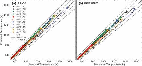
Table 4. The BOL validation metrics for the fuel centerline temperature predictions (Figure 4).

	$d$(K)	$d_M$(K)	$R_2$(–)	RMSE(K)	rRMSE(%)
prior	777.3	14,248.7	0.981	35.3	3.7
present	629.3	10,850.5	0.986	28.6	3.0

4.2. Through-life fuel thermal behavior

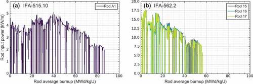
BISON predictions are compared against the experimental data for the selected test cases tabulated in Table 3 from BISON’s assessment test matrix [21]. These cases were specifically chosen to show before and after changes with the proposed model, which were published in Williamson et al. [8]. Figure 5 shows the power histories for the selected Halden Instrumented Fuel Assembly (IFA) cases to be used in the integral-effects validation in Table 3, the four cases are listed for the through-life temperature data for IFA-515.10 (Rod A1) and IFA-562 (Rod 15/16/17) [22,23]. The four cases are composed of annular uranium dioxide fuel pellets which are enclosed by a Zircaloy-2 cladding. The temperature data are acquired by using fuel centerline expansion thermometers. The selected rods are irradiated in the simulations up to high burnups; 75.5GWd/t UO${ }_2$ for IFA-515.10 Rod A1 and approximately 49.4GWd/t UO${ }_2$ for IFA-562.2 rods. To illustrate the results, four different burnup ranges are considered: (a) 0$\le$Bu$<$20, (b) 20$\le$Bu$<$40, (c) 40$\le$Bu$<$60, and (d) Bu$\ge$60 GWd/t UO${ }_2$ [8].

Figure 5. The average linear heat rate histories for (a) the Halden IFA-515.10 irradiation and (b) the Halden IFA-562 irradiation.

Figure 6 shows a comparison of the measured fuel centerline temperatures and the BISON predictions with ‘prior’ and ‘present’ options. With the ‘prior’ option, the BISON predictions are overestimated for IFA-562.2 Rods 15/16/17 and are underestimated for IFA-515.10 Rod A1 against the measurements. As expected, the enhanced gap conductance modeling tends to reduce the fuel centerline temperatures. With the ‘present’ option, the average relative errors are reduced from 83.8 K (7.8%) to 28.7 K (2.7%) for IFA-562.2 Rod 15, from 63.3 K (5.8%) to 13.9 K (1.5%) for IFA-562.2 Rod 16, and from 49.9 K (4.6%) to 14.0 K (1.6%) for IFA-562.2 Rod 17. The relative error is slightly increased from 28.6 K (5.3%) to 34.7 K (6.0%) for IFA-515.10 Rod A1. Overall, the $R^2$-score in Table 5 is improved for the selected test cases, which gets closer to the ideal score of 1.0.

Figure 6. Measured fuel centerline temperatures against the BISON predictions for IFA-515.10 Rod A1, IFA-562.2 Rod 15, IFA-562.2 Rod 16, and IFA-562.2 Rod 17 at four different burnup ranges using (a) Equation (2)(2) $h_{gap}=\frac{{\lambda }_g}{d+{\theta }_1({\xi }_1+{\xi }_2)+(g_1+g_2)}+\frac{{\theta }_2\mathrm{\Lambda }}{\sqrt{{\xi }_1+{\xi }_2}}\left(\frac{W}{H}\right),$(2) with the default modeling options in Table 1 (PRIOR) and (b) Equation (5)(5) $\begin{array}{cc}{h}_{gap}& =\frac{{\lambda }_g}{d+0.605({\xi }_1+{\xi }_2)+(g_1+g_2)}+\frac{10\mathrm{\Lambda }}{\sqrt[4]{0.5({\xi }_1^2+{\xi }_2^2)}}\left(\frac{W}{H}\right),\\ \theta & =\{{\theta }_1,{\theta }_2\}=\left\{0.605,\frac{10.0}{\sqrt[4]{0.5}}\right\}\end{array}$(5) with the new modeling options in Table 1 (PRESENT). The selected rods are irradiated to high burnups; 75.5GWd/t UO${ }_2$ for IFA-515.10 Rod A1 and approximately 49.4GWd/t UO${ }_2$ for IFA-562.2 rods (M = measured; P = predicted). Four different burnup ranges are considered: (1) 0$\le$Bu$<$20, (2) 20$\le$Bu$<$40, (3) 40$\le$Bu$<$60, and (4) Bu$\ge$60 GWd/t UO${ }_2$.

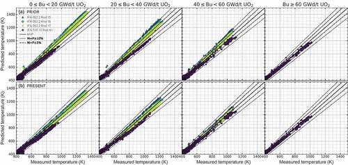
Table 5. The through-life validation metrics for the fuel centerline temperature predictions (Figure 6).

	PRIOR†				PRESENT‡
	R^2	ΔTmax	RMSE	rRMSE	R^2	ΔTmax	RMSE	rRMSE
	(—)	(K)	(K)	(%)	(—)	(K)	(K)	(%)
	IFA-562.2 Rod 15
0≤Bu<20	0.814	126.6	84.2	7.5	0.990	49.1	25.6	2.4
0≤Bu<20	0.830	139.8	90.3	8.6	0.980	69.4	33.9	3.2
40≤Bu<60	0.933	112.1	62.0	6.7	0.988	57.3	24.3	2.7
Overall	0.868	130.6	83.8	7.8	0.988	59.6	28.7	2.7
	IFA-562.2 Rod 16
0≤Bu<20	0.861	113.6	74.7	6.5	0.997	34.2	14.4	1.5
0≤Bu<20	0.917	90.6	57.2	5.3	0.998	35.3	10.7	1.2
40≤Bu<60	0.969	74.7	40.9	4.4	0.997	30.8	11.5	1.4
Overall	0.927	104.1	63.3	5.8	0.997	38.9	13.9	1.5
	IFA-562.2 Rod 17
0≤Bu<20	0.931	94.2	58.9	5.1	0.997	18.0	14.1	1.5
20≤Bu<40	0.964	79.1	44.4	4.2	0.997	28.7	13.7	1.5
40≤Bu<60	0.972	69.6	38.1	4.1	0.998	26.9	10.1	1.3
Overall	0.963	87.5	49.9	4.6	0.997	26.9	14.0	1.6
	IFA-515.10 Rod A1
0≤Bu<20	0.968	48.0	28.9	4.6	0.937	50.6	38.6	5.7
20≤Bu<40	0.976	54.0	27.1	4.8	0.939	60.1	37.5	6.1
40≤Bu<60	0.963	98.1	33.1	8.3	0.964	98.1	32.5	8.1
Bu≥60	0.981	69.1	24.1	5.2	0.982	69.1	23.5	5.2
Overall	0.972	63.9	28.6	5.3	0.953	66.6	34.7	6.0

†Equation (2)(2) $h_{gap}=\frac{{\lambda }_g}{d+{\theta }_1({\xi }_1+{\xi }_2)+(g_1+g_2)}+\frac{{\theta }_2\mathrm{\Lambda }}{\sqrt{{\xi }_1+{\xi }_2}}\left(\frac{W}{H}\right),$(2) with the default modeling options;

‡Equation (5)(5) $\begin{array}{cc}{h}_{gap}& =\frac{{\lambda }_g}{d+0.605({\xi }_1+{\xi }_2)+(g_1+g_2)}+\frac{10\mathrm{\Lambda }}{\sqrt[4]{0.5({\xi }_1^2+{\xi }_2^2)}}\left(\frac{W}{H}\right),\\ \theta & =\{{\theta }_1,{\theta }_2\}=\left\{0.605,\frac{10.0}{\sqrt[4]{0.5}}\right\}\end{array}$(5) with the new modeling options.

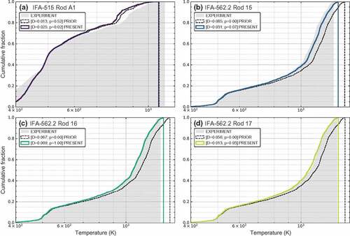
Figure 7 shows the KS-test (Appendix C) results for BISON’s fuel centerline temperature predictions. The cumulative density function (CDF) of the experimental data is shown with the gray-shaded areas. The KS statistics between the experiments and the predictions are provided on the plot for the selected test cases. The results indicate that the null hypothesis cannot be rejected (i.e., the distributions of the two samples are identical) for IFA-562.2 Rods 15/16 with a small KS statistic, $D$, and a high $p$-value. However, there exists a variability between the distributions of the compared two samples with a low $p$-value for both IFA-562.2 Rod 17 and IFA-515.10 Rod A1. For IFA-562.2 Rod 17, the CDF location is slightly shifted towards the high temperatures, and its KS statistics are slightly improved with the ‘present’ option since it moves towards the experiment. For IFA-515.10 Rod A1, both prediction CDFs populate towards the low temperatures as compared to the experiment. As discussed previously, the fuel temperature predictions are underestimated for this specific rod.

Figure 7. KS-test comparison: cumulative fraction plot of the fuel centerline temperature predictions for IFA-515 Rod A1 and IFA-562.2 Rod 15/16/17. The KS statistics are provided on the plot; KS statistic, $D$ – the largest vertical difference between the CDFs of the two samples – and $p$-value. Note that the value of the KS test statistics are not affected by scale changes such as using a log-scale as the test is robust and takes into account only the relative distribution of the data.

4.3. Risø-3

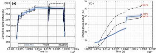
The Risø-3 AN3/4 experiments were conducted at the Risø DR3 water-cooled HP1 rig and utilized a refabricated rod from Biblis, a pressurized water reactor (PWR) [24–26]. For both experiments, the mother rods were irradiated over four reactor cycles up to about 42GWd/t, and refabricated to a shorter length. Both refabricated rods were instrumented with a fuel centerline thermocouple and a pressure transducer. The mother rods are initially filled with helium and pressurized to 2.3 MPa. UO${ }_2$ fuel (93.74% TD) was enriched to 2.95% and was enclosed by Zr-4 cladding. The refabricated rod is filled with helium at 1.5 MPa for Risø-3 AN3 and with xenon at 0.1 MPa for Risø-3 AN4. The aim is to examine the effects of enhanced gap conductance modeling on fuel temperature predictions.

Figures 8 and 9 show the BISON predictions against the experimental data from Risø-3 AN3 and AN4, respectively. The load-to-hardness ratio is estimated to be negligible from the simulations; therefore, the fill gas conductance term dominates the gap conductance in the following benchmarks (i.e., $h_{gap}\propto h_g$). In Figure 8, both BISON simulations underestimate the fuel centerline temperature predictions. In Figure 9, the best agreement is found with the ‘present’ option against the experimental data. As expected, the ‘present’ option tends to reduce the fuel centerline temperature predictions for both cases.

Figure 8. The BISON predictions vs. Risø-3 AN3 measurements for (a) fuel centerline temperature, and (b) fission gas release using the ‘prior’ and ‘present’ options (Grey shaded areas represent a $\pm$5% change around the experimental data.). At EOL, the predicted fission gas release is 26.8% with the ‘prior’ option and 21.0% with the ‘present’ option. Meanwhile, the measured value is 38.3%.

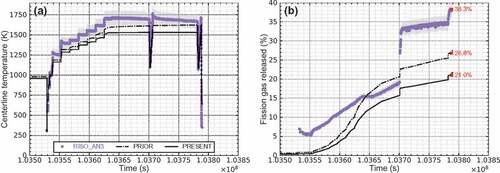
Figure 9. The BISON predictions vs. Risø-3 AN4 measurements for (a) fuel centerline temperature, and (b) fission gas release using the ‘prior’ and ‘present’ options (Grey shaded areas represent a $\pm$5% change around the experimental data.). At EOL, the predicted fission gas release is 54.4% with the ‘prior’ option and 39.7% with the ‘present’ option. Meanwhile, the measured value is 43.0%.

5. Concluding remarks

A new gap conductance model is proposed in this study as a combination of Toptan’s model and the Ross-Stoute model to be representative at high gas pressures and larger contact pressures in nuclear applications. In addition to the proposed gap conductance model, new modeling options (e.g., fill gas thermal conductivity, temperature jump distance, thermal accommodation coefficient, etc.) are added to BISON. To understand how simulation results depend on all input parameters of the proposed model, a variance-based sensitivity analysis is performed at open and closed gap configurations. Then, a series of integral-effects validation tests is performed in BISON at the beginning of life and through-life using the Halden data to ensure that the proposed model is capable of accurately modeling gap heat transfer characteristics in real-world problems. At the beginning of life, the impact of the new gap conductance model is not substantial. The average relative error in centerline temperature predictions reduced from 35.3 K (3.7%) to 28.6 K (3.0%) between BISON’s predictions and measurements. Then, Halden IFA-515.10 (Rod A1) and IFA-562.2 (Rods 15/16/17) through-life rods are used as the integral effects validation. Previously, BISON’s centerline temperature predictions are overestimated for IFA-562.2 Rods 15/16/17 and are underestimated for IFA-515.10 Rod A1 against the measurements. With the proposed modeling, the average relative errors reduced from 83.8 K (7.8%) to 28.7 K (2.7%) for IFA-562.2 Rod 15, from 63.3 K (5.8%) to 13.9 K (1.5%) for IFA-562.2 Rod 16, and from 49.9 K (4.6%) to 14.0 K (1.6%) for IFA-562.2 Rod 17. The relative error is slightly increased from 28.6 K (5.3%) to 34.7 K (6.0%) for IFA-515.10 Rod A1. Lastly, the validation study is extended with Risø-AN3/4 experiments to investigate the impact of adjusted calculation of the fission gas release on fuel temperature predictions using the proposed model. The results indicated that the estimation of the gas composition can impact the temperature predictions, especially as the load-to-hardness ratio approaches zero (i.e., negligible contact conductance). Future work should include a further investigation of the discrepancy for Risø-3 AN3.

Acknowledgments

The submitted manuscript has been authored by a contractor of the U.S. Government under Contract DE-AC07-05ID14517. Accordingly, the U.S. Government retains a non-exclusive, royalty-free license to publish or reproduce the published form of this contribution, or allow others to do so, for U.S. Government purposes.

Disclosure Statement

No potential conflict of interest was reported by the authors.

Appendix A:

Gas density

The behavior of a fluid deviates from that of an ideal gas as its density increases. Many corrections are introduced in the literature, which lead to the virial expansion form of the ideal gas law in terms of the macroscopic thermodynamic properties and particle interactions. The virial equation of state [27,28] is expressed as in Equation (A.1(A.1) $\frac{P}{R_{g}T}=\hat{\rho }+B_2(T){\hat{\rho }}^2+B_3(T){\hat{\rho }}^3,$(A.1) ). If the gas temperature and pressure are known, the density of the gas is computed by solving the cubic equation given in Equation (A.1(A.1) $\frac{P}{R_{g}T}=\hat{\rho }+B_2(T){\hat{\rho }}^2+B_3(T){\hat{\rho }}^3,$(A.1) ), and the density is obtained by employing a root-finding algorithm. Since it is a cubic equation, there may be three possible solutions. The largest real value is assigned for the gas molar density.

(A.1) $\frac{P}{R_{g}T}=\hat{\rho }+B_2(T){\hat{\rho }}^2+B_3(T){\hat{\rho }}^3,$(A.1)

where $P$ is pressure, $T$ is temperature, $R_g$ is ideal gas constant (8.314 J/mol-K), $Z$ is compressibility factor, $\hat{\rho }(=1/V)$ is molar density, and $B_i(T)$ is the $i$–th virial coefficient that is only a function of temperature [19,20].

Roots of the cubic equation The cubic equation with real coefficients is given by

(A.2) $a{x}^3+b{x}^2+cx+d=0,$(A.2)

with $a\ne 0$. This cubic equation is reduced to a monic trinomial (a depressed cubic) using Cardano’s method. The analytical solution can be found in the literature [29]. Roots of the third-order polynomial are computed in the code in the following order (Algorithm 1).

Table

Algorithm 1 Algorithm to find the largest real root of the cubic equation to assign the gas density analytically.

1: procedure

2:     define $\pi =4.0arctan(1.0)$,

3:     initialize $Re=\{0.0\}$ and $Im=\{0.0\}$,

4:     compute $p=\frac{(b^2-3ac)}{9a^2}$; $q=\frac{(9abc-27a^{2}d-2b^3)}{54a^3}$; and $\mathrm{o}\mathrm{f}\mathrm{f}\mathrm{s}\mathrm{e}\mathrm{t}=b/3a$,

5:     compute the discriminant, $\mathrm{\Delta }=(p^3-q^2)$,

6:     if $\mathrm{\Delta }>0$ then

7:        compute $\theta =arccos(q/p\sqrt{p})$ and $r=2\sqrt{p}$

8:        for $n=1,2,3$ do

9:          $Re[n]=r\ast cos\left(\frac{\theta +2(n-1)\pi }{3.0}\right)-\mathrm{o}\mathrm{f}\mathrm{f}\mathrm{s}\mathrm{e}\mathrm{t}$

10:          $Im[n]=0.0$

11:     else

12:        compute ${\gamma }_{1,2}=(q\pm \sqrt{-\mathrm{\Delta }}{)}^{1/3}$

13:        $Re[1]=({\gamma }_1+{\gamma }_2)-\mathrm{o}\mathrm{f}\mathrm{f}\mathrm{s}\mathrm{e}\mathrm{t}$

14:        $Re[2]=Re[3]=-\frac{1}{2}({\gamma }_1+{\gamma }_2)-\mathrm{o}\mathrm{f}\mathrm{f}\mathrm{s}\mathrm{e}\mathrm{t}$

15:        if $\mathrm{\Delta }\ne 0$ then

16:          calculate the complex conjugate roots

17:          $Im[2]=({\gamma }_1+{\gamma }_2)\sqrt{3}2$

18:          $Im[3]=-({\gamma }_1+{\gamma }_2)\sqrt{3}2$

19:     initialize $maxRealRoot=0.0$

20:     for n=1,2,3 do

21:        find the maximum real value

22:        if maxRealRoot $\le Re[n]$ and $Im[n]=0.0$ then

23:          maxRealRoot= $Re[n]$

The hard-coded numerical solution in C++ for the root-finding is compared against the results from the libraries in Python and the expected results. The procedure in Python is relatively easier with the use of numpy libraries. The cubic equation is introduced as roots = np.roots([a, b, c, d]) in the code. The largest real root is computed as maxRealRoot = np.max(roots[np.isreal(roots)]).real. Some examples are provided in Table 6. The results are in good agreement with the expected results.

Table 6. Comparison of the largest real value that is indicated by the bold numerical value. The cubic equation is given by $a{x}^3+b{x}^2+cx+d=0$.

$\{a,b,c,d\}$	Hard-coded in C++	Python	Cubic Eq’n Solver [30]
$\{1,3,3,1\}$	−1.00000	−1.00000 + 5.68937e-6$\cdot$j	−1.0000
		−1.00000–5.68937e-6$\cdot$j
		−1.00001
$\{1,-3,3,-1\}$	1.00000	1.00000 + 5.69146e-6$\cdot$j	1.0000
		1.00000–5.69146e-6$\cdot$j
		1.00001
$\{2,3,-8,3\}$	−3.00000	−3.00000	−3.0000
	0.50000	0.50000	0.5000
	1.00000	1.00000	1.0000
$\{1,5,5,-28\}$	−3.35223 + 2.27817$\cdot$j	−3.35223 + 2.27817$\cdot$j	−3.3522 + 2.2782$\cdot$j
	−3.35223–2.27817$\cdot$j	−3.35223–2.27817$\cdot$j	−3.3522–2.2782$\cdot$j
	1.70446	1.70446	1.7045

Appendix B:

Sobol’ method

Given a random vector $X=\{X_1,\dots ,X_d\}$ where the variables are independent and identically distributed (iid) and the output $Y=f(X)$ of a deterministic model $f$, the functional decomposition of the variance is

(B.1) $\mathrm{V}\mathrm{a}\mathrm{r}(Y)=\sum _{i=1}^d{D}_i(Y)+\sum _{i<j}^d{D}_{ij}(X)+\dots +D_{12\dots d}(Y),$(B.1)

where $D_i(Y)=\mathrm{V}\mathrm{a}\mathrm{r}[\mathbb{E}(Y|X_i)]$, $D_{ij}(Y)=\mathrm{V}\mathrm{a}\mathrm{r}[\mathbb{E}(Y|X_i,X_j)]-D_i(Y)-D_j(Y)$ and similarly for the higher-order interactions.

The Sobol’ indices or variance-based sensitivity indices (Equation B.2a(B.2a) $S_i=\frac{D_i(Y)}{Var(Y)};S_{ij}=\frac{D_{ij}(Y)}{Var(Y)};\dots$(B.2a) ) indicate the share of variance of $Y$ for input or input combination [31]. Total indices (Equation B.2b(B.2b) $S_{T_i}=S_i+\sum _{i<j}{S}_{ij}+\sum _{\genfrac{}{}{0ex}{}{j\ne i}{\genfrac{}{}{0ex}{}{k\ne i}{j<k}}}{S}_{ijk}+\dots =\sum _{l\in \mathrm{\#}i}{S}_l,$(B.2b) ) inform about the model sensitivities [32]. The larger the sensitivity indices, the more critical the parameters are.

(B.2a) $S_i=\frac{D_i(Y)}{Var(Y)};S_{ij}=\frac{D_{ij}(Y)}{Var(Y)};\dots$(B.2a)

(B.2b) $S_{T_i}=S_i+\sum _{i<j}{S}_{ij}+\sum _{\genfrac{}{}{0ex}{}{j\ne i}{\genfrac{}{}{0ex}{}{k\ne i}{j<k}}}{S}_{ijk}+\dots =\sum _{l\in \mathrm{\#}i}{S}_l,$(B.2b)

for $\mathrm{\#}i$ are the all subsets of $\{1,\dots ,d\}$ including $i$. Extensive literature is available for more information on the Sobol’ method in the literature [33–35].

An advantage of the Sobol’ method is providing sensitivity indices of any order of interest. Meanwhile, disadvantages of the method are: (1) requiring specific Monte Carlo sampling [31,36] (i.e., $N=n(d+2)$ in terms of the model calls where $n$ is the size of an initial Monte Carlo sample), and (2) being computationally expensive (e.g., the rate of convergence is $\sqrt{n}$). Note that this study focuses on the sensitivity analysis of a single computational model; therefore, it is adequate and efficient to use this method.

Appendix C:

Kolmogorov–Smirnov Test

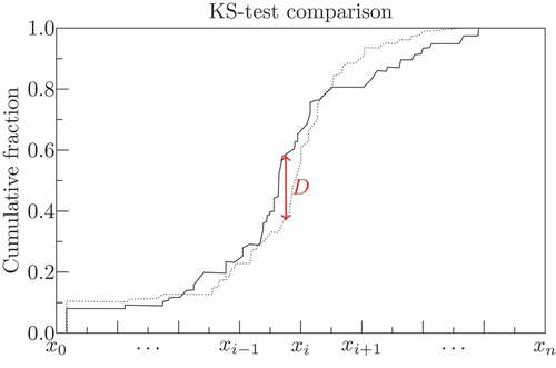
The Kolmogorov–Smirnov (KS) test attempts to determine if two data sets differ significantly in both the location and shape of the cumulative distribution functions (CDFs) of the two samples. The test has the advantage of making no assumption about the distribution of data. It is a non-parametric hypothesis test which measures the probability that a chosen univariate data set is drawn from the same parent population using either a continuous model test (the one-sample KS-test) or a second data set test (the two-sample KS-test). The two-sample KS-test is the primary interest in this study. Kolmogorov [37] and Smirnov [38,39] proved that is the basis for an efficient goodness-of-fit test. The test starts with the definition of the CDF, ${\hat{F}}_n$ for $n$ real numbers $x$. The KS statistics are measures of the supremum distance between the CDFs. The KS statistic $D$ in a two-sample test is

(C.1) $D_{n_1,n_2}=\underset{x}{\mathrm{s}\mathrm{u}\mathrm{p}}\left|{\hat{F}}_{1,n_1}(x)-{\hat{F}}_{2,n_2}(x)\right|,$(C.1)

where $\mathrm{s}\mathrm{u}{\mathrm{p}}_x$ is the supremum of the set of distances, and ${\hat{F}}_{i,n_i}$ is the empirical distribution functions of the $i$-th sample.

The KS test provides a test of a null hypothesis against the alternative hypothesis for two independent samples – given the sequences $x_1={\left\{x_i\right\}}_{i=1}^{n_1}$ and $x_2={\left\{x_i\right\}}_{i=1}^{n_2}$ – with their respective distribution function $F_i(x)$ and the sample CDF ${\hat{F}}_{1,n_i}(x)$ for $i=1,2$. The null hypothesis is a type of hypothesis used in statistics to propose that there is no statistical significance in the given samples (i.e., large KS statistic, $D$, or small $p$-value). Once the KS statistic, $D$, is small, or the $p$-value is high, the null hypothesis – that the distributions of the two samples are identical – cannot be rejected [40]. A schematic illustration of the KS statistic is shown in Figure 10.

Figure 10. Schematic illustration of the Kolmogorov–Smirnov statistic (i.e., the largest vertical difference between the CDFs of the two samples). Note that $p$-value indicates the statistical significance between the two samples.

Appendix D:

Validation metrics

Differences between the observed data (e.g., experimental or expected data) $y=\{y_i{\}}_{i=1}^N$ and the predictions $\tilde{y}=\{{\tilde{y}}_i{\}}_{i=1}^N$ are quantified in terms of the following metrics:

• Euclidean distance, $d(y,\tilde{y})=\sqrt{{\sum }_i^N{\left(y_i-{\tilde{y}}_i\right)}^2}$,

• root-mean-square error, $RMSE=\frac{d(y,\tilde{y})}{\sqrt{N}}$,

• root-mean-square of relative errors, $rRMSE=\frac{d(1,\tilde{y}/y)}{\sqrt{N}}$, and

• coefficient of determination or $R^2$-score, $R^2\equiv 1-\frac{S{S}_{res}}{S{S}_{tot}}$ where the residual and total sum of squares are respectively defined as $S{S}_{res}={\sum }_i^N(y_i-\bar{y}{)}^2$ and $S{S}_{tot}={\sum }_i^N({\tilde{y}}_i-\bar{y}{)}^2$ in terms of the mean of the observed data, $\bar{y}=\frac{1}{N}{\sum }_i^N{y}_i$.

References

- Ross AM, Stoute RL. 1962. Heat transfer coefficient between UO2 and Zircaloy-2. Canada: Atomic Energy of Canada. CRFD-1075: https://inis.iaea.org/collection/NCLCollectionStore/_Public/43/103/43103492.pdf
- Hales JD, et al. BISON theory manual the equations behind nuclear fuel analysis. Idaho Falls (ID): Idaho National Laboratory; 2014.
- Salko R, et al. CTF 4.0 Theory Manual. Oak Ridge (TN): Oak Ridge National Laboratory; 2019. ORNL/TM-2019/1145. doi:10.2172/1550750.
- TRACE V5.0 theory manual field equations, solution methods, and physical models. USA; 2015, DC 20555-0001. [Accessed September 2019] https://www.nrc.gov/docs/ML0710/ML071000097.pdf
- Geelhood K et al. FRAPCON-4.0: A Computer Code for the Calculation of Steady-State, Thermal-Mechanical Behavior of Oxide Fuel Rods for High Burnup. USA; 2015. [Accessed September 2019] https://frapcon.labworks.org/Code-documents/FRAPCON_Description_Final.pdf
- Toptan A, Salko R, Avramova M, et al. A new fuel modeling capability, CTFFuel, with a case study on the fuel thermal conductivity degradation. Nucl Eng Des. 2019;341:248–258.
- Toptan A, Kropaczek D, Avramova M. Gap conductance modeling II: optimized model for UO2-Zircaloy interfaces. Nucl Eng Des. 2019;355:110289.
- Williamson RL, Gamble KA, Pereza DM, et al. Validating the BISON fuel performance code to integral LWR experiments. Nucl Eng Des. 2016;301:232–244.
- Bird RB, Stewart WE, Lightfoot EN. Transport Phenomena. New York: John Wiley and Sons, Inc.; 1960.
- Toptan A. A novel approach to improve transient fuel performance modeling in multi-physics calculations. Raleigh (NC): North Carolina State University, Nuclear Engineering; 2019. https://repository.lib.ncsu.edu/handle/1840.20/36352
- Garnier JE, Begej S. Ex-reactor determination of thermal gap conductance between uranium dioxide and Zircaloy-4 – stage II: high gas pressure. USA: Pacific Northwest Laboratory; 1980. NUREG/CR-0330; PNL-3232. doi:10.2172/1076471.
- Toptan A, Kropaczek D, Avramova M. Gap conductance modeling I: theoretical considerations for single- and multi-component gases in curvilinear coordinates. Nucl Eng Des. 2019;353:110283.
- Hagrman DL, Reymann GA, Manson RE. MATPRO-version 11 (rev. 1): a handbook of materials properties for use in the analysis of light water reactor fuel rod behavior. Idaho Falls (ID): Idaho National Engineering Laboratory; 1980. NUREG/CR-0497, TREE-1290. doi:10.2172/6442256.
- Lanning DD, Hann CR. Review of review of methods applicable to the calculation of gap conductance in Zircaloy-Clad UO2 fuel rods. USA: Pacific Northwest Laboratory; 1975. BNWL-1894. doi:10.2172/4209005.
- Jacobs G, Todreas N. Thermal contact conductance in reactor fuel elements. Nucl Sci Eng. 1973;50(3):283–306.
- Oberkampf WL, Roy CJ. Verification and validation in scientific computing. Cambridge, UK: Cambridge University Press; 2010.
- Hann C, Lanning D, Bradley E, et al. Data report for the NRC/PNL Halden assembly IFA-432. PNL, 1978, NUREG/CR-0560; PNL-2673. doi:10.2172/6401826.
- Sartori E, Killeen J, Turnbull J International fuel performance experiments (IFPE) database. OECD-NEA, 2010. [Accessed September 2019] Available at www.oecd-nea.org/science/fuel/ifpelst.html.
- Tournier J-MP, El-Genk MS. Properties of noble gases and binary mixtures for closed brayton cycle applications. Energy Convers Manag. 2008;49(3):469–492.
- Toptan A, Kropaczek D, Avramova M. On the validity of the dilute gas assumption for gap conductance calculations in nuclear fuel performance codes. Nucl Eng Des. 2019;350:1–8.
- BISON Team. Assessment of BISON: a nuclear fuel performance analysis code. USA: Idaho National Laboratory, Fuels Modeling and Simulation Department; 2017. INL/MIS-13-30314.
- Tverberg T, Amaya M. Study of thermal behaviour of UO2 and (U,Gd)O2 to high burnup (IFA-515). Norway: OECD Halden Reactor Project; 2001. ( HWR-671).
- Lösönen P. Early-in-life Irradiation of IFA-562.2 (the ultra high burn-up experiment). Norway: OECD Halden Reactor Project; 1989. ( HWR-247).
- Fuel modelling at extended burnup (FUMEX-II): report of a coordinated research project. International Atomic Energy Agency, 2002-2007, IAEA-TECDOC-1687.
- The third Risø fission gas project: bump test AN2 (CB6). Risø, 1990, Risø-FGP3-AN2, Risø.
- The third Risø fission gas project: bump test AN4 (CB7-2R). Risø, 1990, Risø-FGP3-AN4.
- Onnes HK. Expression of the equation of state of gases and liquids by means of series, in Koninklijke Nederlandse Akademie van Wetenschappen. Proc Ser B Phys Sci. 1901;4:125–147.
- Mason EA, Spurling TH. The virial equation of state. Toronto: Pergamon Press; 1969.
- Weisstein EW “Cubic Formula.” from mathworld–a wolfram web resource. [ Online; cited 2019 Aug 8]. Available at http://mathworld.wolfram.com/cubicformula.html
- Wolfram—alpha widgets: cubic equation solver. [ Online; cited 2019 Dec 5]. Available at https://www.wolframalpha.com/widgets/view.jsp?id=1beb192fcbfba3b6afa17b00ae68605a
- Sobol’ I. Sensitivity estimates for nonlinear mathematical models. Math Modell Comput Exp. 1993(1):404–414.
- Homma T, Saltelli A. Importance measures in global sensitivity analysis of non linear models. Reliab Eng Syst Saf. 1996;52(1):1–17.
- Iooss B, Lemaître P. A review on global sensitivity analysis methods. Boston, MA: Springer; 2015. DOI:10.1007/978-1-4899-7547-8_5.
- Herman J, Usher W. Salib: an open-source python library for sensitivity analysis. The Journal of Open Source Software. 2017;2(9):97.
- Smith R Uncertainly Quantification: theory, Implementation, and Applications. SIAM in the Computational Science and Engineering Series, CS12; 2014.
- Saltelli A. Making best use of model evaluations to compute sensitivity indices. Comput Phys Commun. 2002;145(2):280–297.
- Kolmogorov AN. Sulla Determinazione Empirica di una Legge di Distribuzione. Giornale dell’Istituto Italiano degli Attuari. 1933;4:83–91.
- Smirnov NV. On the estimation of the discrepancy between empirical curves of distribution for two independent samples. Bull Math l’Universite Moscou. 1939;2:3–16.
- Smirnov NV Table for estimating the goodness of fit of empirical distributions. Ann Math Stat. 1948;19(2):279–281. https://doi.org/10.1214/aoms/1177730256
- Jones E, Oliphant T, Peterson P, et al. SciPy: open source scientific tools for Python. 2001. [ Online; cited 2019 Dec 5]. Available at http://www.scipy.org