Novel approach to solving the inverse equation of point kinetics by the Bernoulli number generalisation method

ABSTRACT

A new approach to solve the inverse equation of point kinetics is presented. The neutron density history can be considered as a series of infinite Bernoulli numbers. In order to simplify the problem, the proposed method uses an approximation which considers only two derivatives of the neutron population density. The reactivity is calculated for different forms of neutron population density and for different time steps. Due to its high precision, the results obtained suggest that the proposed method can be used in a real-time digital reactivity meter.

KEYWORDS:

• Reactivity
• nuclear power plant
• nuclear reactor
• numerical simulation
• inverse equation of point kinetics
• infinite Bernoulli numbers
• Euler–Maclaurin formula

1. Introduction

In order to safely control a nuclear power station, it is necessary to know the value of the reactivity with the highest precision, this value is known from the population density of neutrons that depends on the fission interaction of different materials [1].

A great variety of scientific works have been carried out around the calculation of the reactivity, each of which proposes a different solution method, in the quest for both a better approximation and low computational cost. The reported works [2–7] determine the reactivity and the neutron source, taking into account sub-critical conditions for the neutron population density. Another method, that determines the reactivity without the dependence on the history of neutron population density was proposed [8], where the reactivity term was modified to solely depend on the derivatives of the neutron population. Later on, a method that uses the discrete version of the Laplace transform – which was implemented in a non-recursive way in what is known as the FIR filter – was proposed [9]. This method allows the discretisation of the integral of the history of neutron population density in a convolution sum, but with a significant computational cost. Another method that uses a Lagrangian polynomial form [10] with an accuracy of $O\left(h^n\right)$ was proposed, but with the drawback that if the order of the polynomial is increased, the computational cost is also increased. Subsequently, a method based on the Euler–Maclaurin formula was published where the first Bernoulli number was used as an approximation [11], this approximation increased the accuracy in the calculation of nuclear reactivity. Recently, a paper with a very good accuracy in the calculation of reactivity was reported, it is based on a matrix formulation for the calculation of reactivity [12]. For this work, a new approach is proposed for the integral of the history of neutron population density by means of an infinite sum containing the Bernoulli numbers.

This work’s motivation mainly points out to state that there are currently two methods with very good accuracy for the calculation of reactivity and they were named above, such as the method of derivatives (DM) [8] and the matrix formulation method (MF) [12]. The latter method demonstrated superiority in accuracy over the former, because it has no restrictions on the shape of neutron density, but has a higher computational cost since it requires multiplication of matrices. However, the matrix formulation method (MF) is accurate and fast enough to be implemented in real-time digital reactivity meters.

The objective of this work is to provide an alternative method to the matrix formulation (MF) method that has equal or greater accuracy in the calculation of reactivity, although the proposed method uses restrictions in the form of neutron density as in the derivative method (DM). To validate the proposed method, different numerical experiments with different forms of neutron density distributed in eight cases were performed.

This article is organized in the following way: in Section 2 the inverse equation of point kinetics is deduced. In Section 2.1 the reactivity is calculated using the first two Bernoulli numbers. In Section 3 the proposed method for reactivity with the generalisation of the Bernoulli numbers is developed; in Section 4 the results are shown, and finally, in Section 5 the conclusions are given.

2. Inverse equation of point kinetics

The equations that model the dynamics of a nuclear reactor are known as the equations of point kinetics, which can be obtained from the neutron diffusion equation. These equations describe the time evolution of the neutron distribution and the concentration of delayed neutron precursors [1]:

(1) $\frac{dP(t)}{dt}=\left[\frac{\rho (t)-\beta }{\mathrm{\Lambda }}\right]P(t)+\sum _{i=1}^6{\lambda }_i{C}_i(t)$(1)

(2) $\frac{d{C}_i(t)}{dt}+{\lambda }_i{C}_i(t)=\frac{{\beta }_i}{\mathrm{\Lambda }}P(t);i=1,2,...,6$(2)

With initial conditions:

(3) $P(t=0)=P_0$(3)

(4) $C_i(t=0)=\frac{{\beta }_i}{\mathrm{\Lambda }{\lambda }_i}{P}_0$(4)

where $C_i(t)$ is the concentration of the ith group of delayed neutron precursors, $P(t)$ is the density of the neutron population, $\rho (t)$ is the reactivity, $\mathrm{\Lambda }$ is the neutron generation time, ${\beta }_i$ is the ith fraction of delayed neutrons, $\beta$ is the total effective fraction of delayed neutrons and ${\lambda }_i$ is the decay constant of the ith group of delayed neutron precursors.

It is possible to solve Equation (2)(2) $\frac{d{C}_i(t)}{dt}+{\lambda }_i{C}_i(t)=\frac{{\beta }_i}{\mathrm{\Lambda }}P(t);i=1,2,...,6$(2) using the integrating factor method and making use of the initial conditions (3) and (4), thus obtaining an expression for the concentration of precursors of the ith group of delayed neutrons:

(5) $C_i(t)=\frac{{\beta }_i}{\mathrm{\Lambda }}\left[\frac{e^{-{\lambda }_{i}t}}{{\lambda }_i}{P}_0+\underset{0}{\overset{t}{\int }}{e}^{-{\lambda }_i(t-t^{\prime })}P(t^{\prime })d{t}^{\prime }\right]$(5)

Now, isolating $\rho (t)$in Equation (1)(1) $\frac{dP(t)}{dt}=\left[\frac{\rho (t)-\beta }{\mathrm{\Lambda }}\right]P(t)+\sum _{i=1}^6{\lambda }_i{C}_i(t)$(1) we get an expression for the reactivity:

(6) $\rho (t)=\beta +\frac{\mathrm{\Lambda }}{P(t)}\frac{dP(t)}{dt}-\frac{\mathrm{\Lambda }}{P(t)}\sum _{i=1}^6{\lambda }_i{C}_i(t)$(6)

By replacing Equation (5)(5) $C_i(t)=\frac{{\beta }_i}{\mathrm{\Lambda }}\left[\frac{e^{-{\lambda }_{i}t}}{{\lambda }_i}{P}_0+\underset{0}{\overset{t}{\int }}{e}^{-{\lambda }_i(t-t^{\prime })}P(t^{\prime })d{t}^{\prime }\right]$(5) into Equation (6)(6) $\rho (t)=\beta +\frac{\mathrm{\Lambda }}{P(t)}\frac{dP(t)}{dt}-\frac{\mathrm{\Lambda }}{P(t)}\sum _{i=1}^6{\lambda }_i{C}_i(t)$(6) we get:

(7) $\rho (t)=\beta +\frac{\mathrm{\Lambda }}{P(t)}\frac{dP(t)}{dt}-\frac{P(0)}{P(t)}\sum _{i=1}^6{\beta }_i{e}^{-{\lambda }_{i}t}\text{break}-\frac{1}{P(t)}\sum _{i=1}^6\underset{0}{\overset{t}{\int }}{\lambda }_i{\beta }_i{e}^{-{\lambda }_i(t-t^{\prime })}P(t^{\prime })d{t}^{\prime }$(7)

Equation (7)(7) $\rho (t)=\beta +\frac{\mathrm{\Lambda }}{P(t)}\frac{dP(t)}{dt}-\frac{P(0)}{P(t)}\sum _{i=1}^6{\beta }_i{e}^{-{\lambda }_{i}t}\text{break}-\frac{1}{P(t)}\sum _{i=1}^6\underset{0}{\overset{t}{\int }}{\lambda }_i{\beta }_i{e}^{-{\lambda }_i(t-t^{\prime })}P(t^{\prime })d{t}^{\prime }$(7) represents the inverse equation of point kinetics and it is the basis for the construction of digital on-line reactivity meters [13]. This equation is not used directly in the calculation of reactivity because it presents difficulties due to the computational cost in real-time measurements.

2.1. Euler–Maclaurin identity for the calculation of reactivity

In this section, two approximations for the integral in Equation (7)(7) $\rho (t)=\beta +\frac{\mathrm{\Lambda }}{P(t)}\frac{dP(t)}{dt}-\frac{P(0)}{P(t)}\sum _{i=1}^6{\beta }_i{e}^{-{\lambda }_{i}t}\text{break}-\frac{1}{P(t)}\sum _{i=1}^6\underset{0}{\overset{t}{\int }}{\lambda }_i{\beta }_i{e}^{-{\lambda }_i(t-t^{\prime })}P(t^{\prime })d{t}^{\prime }$(7) for the calculation of reactivity using the first two Bernoulli numbers are presented, which will allow us to observe a repetitive behavior that helps us obtain a general formula that includes the infinite Bernoulli numbers.

In order to solve the integral that appears in Equation (7)(7) $\rho (t)=\beta +\frac{\mathrm{\Lambda }}{P(t)}\frac{dP(t)}{dt}-\frac{P(0)}{P(t)}\sum _{i=1}^6{\beta }_i{e}^{-{\lambda }_{i}t}\text{break}-\frac{1}{P(t)}\sum _{i=1}^6\underset{0}{\overset{t}{\int }}{\lambda }_i{\beta }_i{e}^{-{\lambda }_i(t-t^{\prime })}P(t^{\prime })d{t}^{\prime }$(7) , the Euler–Maclaurin formula [11] is used:

(8) $\underset{0}{\overset{n}{\int }}F(k)dk=\sum _{m=1}^{n-1}F[m]+\frac{1}{2}\left[F[0]+F[n]\right]\text{break}-\sum _{p=1}^{\mathrm{\infty }}{(-1)}^{p-1}\frac{B_p}{(2p)!}\left[F^{(2p-1)}[n]-F^{(2p-1)}[0]\right]$(8)

where the $B_p$ are the Bernoulli numbers shown in Table 1.

Table 1. First Bernoulli numbers.

${\mathbf{B}}_1=1/6$	${\mathbf{B}}_5=5/66$	${\mathbf{B}}_9=43867/798$
${\mathbf{B}}_2=1/30$	${\mathrm{B}}_6=691/2730$	${\mathrm{B}}_{10}=174611/330$
${\mathbf{B}}_3=1/42$	${\mathrm{B}}_7=7/6$	${\mathrm{B}}_{11}=854513/138$
${\mathbf{B}}_4=1/30$	${\mathrm{B}}_8=3617/510$	${\mathrm{B}}_{12}=236364091/2730$

It is possible to simplify the integrand of Equation (7)(7) $\rho (t)=\beta +\frac{\mathrm{\Lambda }}{P(t)}\frac{dP(t)}{dt}-\frac{P(0)}{P(t)}\sum _{i=1}^6{\beta }_i{e}^{-{\lambda }_{i}t}\text{break}-\frac{1}{P(t)}\sum _{i=1}^6\underset{0}{\overset{t}{\int }}{\lambda }_i{\beta }_i{e}^{-{\lambda }_i(t-t^{\prime })}P(t^{\prime })d{t}^{\prime }$(7) by doing the following:

(9) $h_i(t-t^{\prime })={\lambda }_i{\beta }_i{e}^{-{\lambda }_i(t-t^{\prime })}$(9)

Equation (9)(9) $h_i(t-t^{\prime })={\lambda }_i{\beta }_i{e}^{-{\lambda }_i(t-t^{\prime })}$(9) represents the continuous response of the system to a unit impulse function [14]. With this response and the neutron population density in the integrand in Equation (7)(7) $\rho (t)=\beta +\frac{\mathrm{\Lambda }}{P(t)}\frac{dP(t)}{dt}-\frac{P(0)}{P(t)}\sum _{i=1}^6{\beta }_i{e}^{-{\lambda }_{i}t}\text{break}-\frac{1}{P(t)}\sum _{i=1}^6\underset{0}{\overset{t}{\int }}{\lambda }_i{\beta }_i{e}^{-{\lambda }_i(t-t^{\prime })}P(t^{\prime })d{t}^{\prime }$(7) , it can be obtained:

(10) $F(t^{\prime })=h_i(t-t^{\prime })P(t^{\prime })$(10)

The discrete version of Equation (10)(10) $F(t^{\prime })=h_i(t-t^{\prime })P(t^{\prime })$(10) can be written in the form:

(11) $F[m]=h_i[n-m]P[m]$(11)

making $p=1$ in Equation (8)(8) $\underset{0}{\overset{n}{\int }}F(k)dk=\sum _{m=1}^{n-1}F[m]+\frac{1}{2}\left[F[0]+F[n]\right]\text{break}-\sum _{p=1}^{\mathrm{\infty }}{(-1)}^{p-1}\frac{B_p}{(2p)!}\left[F^{(2p-1)}[n]-F^{(2p-1)}[0]\right]$(8) and making use of Equation (11)(11) $F[m]=h_i[n-m]P[m]$(11) , it is possible to show that Equation (7)(7) $\rho (t)=\beta +\frac{\mathrm{\Lambda }}{P(t)}\frac{dP(t)}{dt}-\frac{P(0)}{P(t)}\sum _{i=1}^6{\beta }_i{e}^{-{\lambda }_{i}t}\text{break}-\frac{1}{P(t)}\sum _{i=1}^6\underset{0}{\overset{t}{\int }}{\lambda }_i{\beta }_i{e}^{-{\lambda }_i(t-t^{\prime })}P(t^{\prime })d{t}^{\prime }$(7) can be written as [11]:

(12) $\begin{array}{rl}& \rho \left[n\right]=\beta +\frac{\mathrm{\Lambda }}{P[n]}{P}^{(1)}[n]-\frac{P_0}{P[n]}\sum _{i=1}^6{\beta }_i{e}^{-{\lambda }_{i}nT}\\ & -\frac{T}{P[n]}\sum _{i=1}^6\left[\sum _{m=0}^n{h}_i[n-m]P[m]\right.\\ & \left.-\frac{1}{2}[h_i[n]P[0]+h_i[0]P[n]]\right]\\ & +\frac{T^2}{12P[n]}\sum _{i=1}^6[{h_i}^{(1)}[0]P[n]+h_i[0]P^{(1)}[n]\\ & -{h_i}^{(1)}[n]P[0]-h_i[n]P^{(1)}[0]]\end{array}$(12)

where time is discretised as

(13) $t=nT$(13)

Being T the time step in the reactivity calculation, $n\ge 0,n\in \mathbb{Z}$, that is n is a non-negative integer. Equation (13)(13) $t=nT$(13) allows to go from a continuous time to a discrete one.

It is possible to find an expression for the second Bernoulli number, by making $p=2$in Equation (8)(8) $\underset{0}{\overset{n}{\int }}F(k)dk=\sum _{m=1}^{n-1}F[m]+\frac{1}{2}\left[F[0]+F[n]\right]\text{break}-\sum _{p=1}^{\mathrm{\infty }}{(-1)}^{p-1}\frac{B_p}{(2p)!}\left[F^{(2p-1)}[n]-F^{(2p-1)}[0]\right]$(8) . Equations (9)(9) $h_i(t-t^{\prime })={\lambda }_i{\beta }_i{e}^{-{\lambda }_i(t-t^{\prime })}$(9) and (11(11) $F[m]=h_i[n-m]P[m]$(11) ) are derived three times to obtain:

(14) $\begin{array}{rl}& F^{(3)}[m]=h_i^{(3)}[n-m]P[m]+3(h_i^{(2)}[n-m]P^{(1)}[m])\\ & +3(h_i^{(1)}[n-m]P^{(2)}[m])+h_i[n-m]P^{(3)}[m]\end{array}$(14)

Making $m=n$ in Equation (14)(14) $\begin{array}{rl}& F^{(3)}[m]=h_i^{(3)}[n-m]P[m]+3(h_i^{(2)}[n-m]P^{(1)}[m])\\ & +3(h_i^{(1)}[n-m]P^{(2)}[m])+h_i[n-m]P^{(3)}[m]\end{array}$(14) we get:

(15) $\begin{array}{rl}& F^{(3)}[n]=h_i^{(3)}[0]P[n]+3(h_i^{(2)}[0]P^{(1)}[n])\\ & +3(h_i^{(1)}[0]P^{(2)}[n])+h_i[0]P^{(3)}[n]r\end{array}$(15)

Making $m=0$ in Equation (14)(14) $\begin{array}{rl}& F^{(3)}[m]=h_i^{(3)}[n-m]P[m]+3(h_i^{(2)}[n-m]P^{(1)}[m])\\ & +3(h_i^{(1)}[n-m]P^{(2)}[m])+h_i[n-m]P^{(3)}[m]\end{array}$(14) we get:

(16) $\begin{array}{rl}& F^{(3)}[0]=h_i^{(3)}[n]P[0]+3(h_i^{(2)}[n]P^{(1)}[0])\\ & +3(h_i^{(1)}[n]P^{(2)}[0])+h_i[n]P^{(3)}[0]\end{array}$(16)

Subtracting Equation (15)(15) $\begin{array}{rl}& F^{(3)}[n]=h_i^{(3)}[0]P[n]+3(h_i^{(2)}[0]P^{(1)}[n])\\ & +3(h_i^{(1)}[0]P^{(2)}[n])+h_i[0]P^{(3)}[n]r\end{array}$(15) from Equation (16)(16) $\begin{array}{rl}& F^{(3)}[0]=h_i^{(3)}[n]P[0]+3(h_i^{(2)}[n]P^{(1)}[0])\\ & +3(h_i^{(1)}[n]P^{(2)}[0])+h_i[n]P^{(3)}[0]\end{array}$(16) we get,

(17) $\begin{array}{rl}& F^{(3)}[n]-F^{(3)}[0]\\ & =\left[\begin{array}{c}{h}_i^{(3)}[0]P[n]+3(h_i^{(2)}[0]P^{(1)}[n])+3(h_i^{(1)}[0]P^{(2)}[n])\\ +h_i[0]P^{(3)}[n]\end{array}\right]\\ & -\left[\begin{array}{c}{h}_i^{(3)}[n]P[0]+3(h_i^{(2)}[n]P^{(1)}[0])+3(h_i^{(1)}[n]P^{(2)}[0])\\ +h_i[n]P^{(3)}[0]\end{array}\right]\end{array}$(17)

By replacing Equation (17)(17) $\begin{array}{rl}& F^{(3)}[n]-F^{(3)}[0]\\ & =\left[\begin{array}{c}{h}_i^{(3)}[0]P[n]+3(h_i^{(2)}[0]P^{(1)}[n])+3(h_i^{(1)}[0]P^{(2)}[n])\\ +h_i[0]P^{(3)}[n]\end{array}\right]\\ & -\left[\begin{array}{c}{h}_i^{(3)}[n]P[0]+3(h_i^{(2)}[n]P^{(1)}[0])+3(h_i^{(1)}[n]P^{(2)}[0])\\ +h_i[n]P^{(3)}[0]\end{array}\right]\end{array}$(17) into Equation (8)(8) $\underset{0}{\overset{n}{\int }}F(k)dk=\sum _{m=1}^{n-1}F[m]+\frac{1}{2}\left[F[0]+F[n]\right]\text{break}-\sum _{p=1}^{\mathrm{\infty }}{(-1)}^{p-1}\frac{B_p}{(2p)!}\left[F^{(2p-1)}[n]-F^{(2p-1)}[0]\right]$(8) we get:

(18) $\begin{array}{rl}& \underset{0}{\overset{t}{\int }}F(k)dk=\underset{0}{\overset{t}{\int }}{h}_i(t-t^{\prime })P(t^{\prime })d{t}^{\prime }=T\left[\sum _{m=0}^n{h}_i[n-m]P[m]\right.\\ & \left.-\frac{1}{2}[h_i[n]P[0]+h_i[0]P[n]]\right]\\ & -\frac{T^2}{12}[{h_i}^{(1)}[0]P[n]+h_i[0]P^{(1)}[n]\\ & -{h_i}^{(1)}[n]P[0]+h_i[n]P^{(1)}[0]]\\ & +\frac{T^4}{720}[{h_i}^{(3)}[0]P[n]+3({h_i}^{(2)}[0]P^{(1)}[n])\\ & +3({h_i}^{(1)}[0]P^{(2)}[n])+h_i[0]P^{(3)}[n]\\ & -{h_i}^{(3)}[n]P[0]-3({h_i}^{(2)}[n]P^{(1)}[0])\\ & -3({h_i}^{(1)}[n]P^{(2)}[0])-h_i[n]P^{(3)}[0]]\end{array}$(18)

By replacing Equation (18)(18) $\begin{array}{rl}& \underset{0}{\overset{t}{\int }}F(k)dk=\underset{0}{\overset{t}{\int }}{h}_i(t-t^{\prime })P(t^{\prime })d{t}^{\prime }=T\left[\sum _{m=0}^n{h}_i[n-m]P[m]\right.\\ & \left.-\frac{1}{2}[h_i[n]P[0]+h_i[0]P[n]]\right]\\ & -\frac{T^2}{12}[{h_i}^{(1)}[0]P[n]+h_i[0]P^{(1)}[n]\\ & -{h_i}^{(1)}[n]P[0]+h_i[n]P^{(1)}[0]]\\ & +\frac{T^4}{720}[{h_i}^{(3)}[0]P[n]+3({h_i}^{(2)}[0]P^{(1)}[n])\\ & +3({h_i}^{(1)}[0]P^{(2)}[n])+h_i[0]P^{(3)}[n]\\ & -{h_i}^{(3)}[n]P[0]-3({h_i}^{(2)}[n]P^{(1)}[0])\\ & -3({h_i}^{(1)}[n]P^{(2)}[0])-h_i[n]P^{(3)}[0]]\end{array}$(18) into Equation (7)(7) $\rho (t)=\beta +\frac{\mathrm{\Lambda }}{P(t)}\frac{dP(t)}{dt}-\frac{P(0)}{P(t)}\sum _{i=1}^6{\beta }_i{e}^{-{\lambda }_{i}t}\text{break}-\frac{1}{P(t)}\sum _{i=1}^6\underset{0}{\overset{t}{\int }}{\lambda }_i{\beta }_i{e}^{-{\lambda }_i(t-t^{\prime })}P(t^{\prime })d{t}^{\prime }$(7) we get:

(19) $\begin{array}{rl}& \rho \left[n\right]={\rho }_{FIR}[n]+\frac{T^2}{12P[n]}\sum _{i=1}^6\left[{h_i}^{(1)}[0]P[n]+h_i[0]P^{(1)}[n]\right.\\ & \left.-{h_i}^{(1)}[n]P[0]-h_i[n]P^{(1)}[0]\right]\\ & -\frac{T^4}{720P[n]}\sum _{i=1}^6\left[\begin{array}{c}{h_i}^{(3)}[0]P[n]+3({h_i}^{(2)}[0]P^{(1)}[n])\\ +3({h_i}^{(1)}[0]P^{(2)}[n])+h_i[0]P^{(3)}[n]\\ -{h_i}^{(3)}[n]P[0]-3({h_i}^{(2)}[n]P^{(1)}[0])\\ -3({h_i}^{(1)}[n]P^{(2)}[0])-h_i[n]P^{(3)}[0]\end{array}\right]\end{array}$(19)

where

(20) $\begin{array}{rl}& {\rho }_{FIR}\left[n\right]=\beta +\frac{\mathrm{\Lambda }}{P[n]}{P}^{(1)}[n]-\frac{P_0}{P[n]}\sum _{i=1}^6{\beta }_i{e}^{-{\lambda }_{i}nT}\\ & -\frac{T}{P[n]}\sum _{i=1}^6\left[\sum _{m=0}^n{h}_i[n-m]P[m]\right.\\ & \left.-\frac{1}{2}\left[h_i[n]P[0]+h_i[0]P[n]\right]\right]\end{array}$(20)

Equation (19)(19) $\begin{array}{rl}& \rho \left[n\right]={\rho }_{FIR}[n]+\frac{T^2}{12P[n]}\sum _{i=1}^6\left[{h_i}^{(1)}[0]P[n]+h_i[0]P^{(1)}[n]\right.\\ & \left.-{h_i}^{(1)}[n]P[0]-h_i[n]P^{(1)}[0]\right]\\ & -\frac{T^4}{720P[n]}\sum _{i=1}^6\left[\begin{array}{c}{h_i}^{(3)}[0]P[n]+3({h_i}^{(2)}[0]P^{(1)}[n])\\ +3({h_i}^{(1)}[0]P^{(2)}[n])+h_i[0]P^{(3)}[n]\\ -{h_i}^{(3)}[n]P[0]-3({h_i}^{(2)}[n]P^{(1)}[0])\\ -3({h_i}^{(1)}[n]P^{(2)}[0])-h_i[n]P^{(3)}[0]\end{array}\right]\end{array}$(19) represents the reactivity with two Bernoulli numbers. In the next section, we present the proposed method to find a general formula for the calculation of reactivity that can reproduce particular cases with one or two Bernoulli numbers.

3. Proposed method

A relationship with the Pascal’s triangle can be seen for each one of the terms in Equation (19)(19) $\begin{array}{rl}& \rho \left[n\right]={\rho }_{FIR}[n]+\frac{T^2}{12P[n]}\sum _{i=1}^6\left[{h_i}^{(1)}[0]P[n]+h_i[0]P^{(1)}[n]\right.\\ & \left.-{h_i}^{(1)}[n]P[0]-h_i[n]P^{(1)}[0]\right]\\ & -\frac{T^4}{720P[n]}\sum _{i=1}^6\left[\begin{array}{c}{h_i}^{(3)}[0]P[n]+3({h_i}^{(2)}[0]P^{(1)}[n])\\ +3({h_i}^{(1)}[0]P^{(2)}[n])+h_i[0]P^{(3)}[n]\\ -{h_i}^{(3)}[n]P[0]-3({h_i}^{(2)}[n]P^{(1)}[0])\\ -3({h_i}^{(1)}[n]P^{(2)}[0])-h_i[n]P^{(3)}[0]\end{array}\right]\end{array}$(19) . In order to find a method for calculating the reactivity with any Bernoulli number, the binomial theorem can be used to obtain a given order for the derivatives of the system’s response to a unit impulse function. It is possible to express Equations (12)(12) $\begin{array}{rl}& \rho \left[n\right]=\beta +\frac{\mathrm{\Lambda }}{P[n]}{P}^{(1)}[n]-\frac{P_0}{P[n]}\sum _{i=1}^6{\beta }_i{e}^{-{\lambda }_{i}nT}\\ & -\frac{T}{P[n]}\sum _{i=1}^6\left[\sum _{m=0}^n{h}_i[n-m]P[m]\right.\\ & \left.-\frac{1}{2}[h_i[n]P[0]+h_i[0]P[n]]\right]\\ & +\frac{T^2}{12P[n]}\sum _{i=1}^6[{h_i}^{(1)}[0]P[n]+h_i[0]P^{(1)}[n]\\ & -{h_i}^{(1)}[n]P[0]-h_i[n]P^{(1)}[0]]\end{array}$(12) and (19(19) $\begin{array}{rl}& \rho \left[n\right]={\rho }_{FIR}[n]+\frac{T^2}{12P[n]}\sum _{i=1}^6\left[{h_i}^{(1)}[0]P[n]+h_i[0]P^{(1)}[n]\right.\\ & \left.-{h_i}^{(1)}[n]P[0]-h_i[n]P^{(1)}[0]\right]\\ & -\frac{T^4}{720P[n]}\sum _{i=1}^6\left[\begin{array}{c}{h_i}^{(3)}[0]P[n]+3({h_i}^{(2)}[0]P^{(1)}[n])\\ +3({h_i}^{(1)}[0]P^{(2)}[n])+h_i[0]P^{(3)}[n]\\ -{h_i}^{(3)}[n]P[0]-3({h_i}^{(2)}[n]P^{(1)}[0])\\ -3({h_i}^{(1)}[n]P^{(2)}[0])-h_i[n]P^{(3)}[0]\end{array}\right]\end{array}$(19) ) in the following way:

(21) $\begin{array}{rl}& \rho \left[n\right]={\rho }_{FIR}[n]\\ & +\frac{1}{P[n]}\sum _{i=1}^6\left[\sum _{p=1}^{\mathrm{\infty }}{(-1)}^{p-1}\frac{T^{2p}{B}_p}{(2p)!}\right.\\ & \left.\left[\begin{array}{c}\sum _{k=0}^{2p-1}\left(\begin{array}{c}2p-1\\ k\end{array}\right){h_i}^{(2p-k-1)}[0]P^{(k)}[n]\\ -\sum _{k=0}^{2p-1}\left(\begin{array}{c}2p-1\\ k\end{array}\right){h_i}^{(2p-k-1)}[n]P^{(k)}[0]\end{array}\right]\right]\end{array}$(21)

The summation of binomial terms in Equation (21)(21) $\begin{array}{rl}& \rho \left[n\right]={\rho }_{FIR}[n]\\ & +\frac{1}{P[n]}\sum _{i=1}^6\left[\sum _{p=1}^{\mathrm{\infty }}{(-1)}^{p-1}\frac{T^{2p}{B}_p}{(2p)!}\right.\\ & \left.\left[\begin{array}{c}\sum _{k=0}^{2p-1}\left(\begin{array}{c}2p-1\\ k\end{array}\right){h_i}^{(2p-k-1)}[0]P^{(k)}[n]\\ -\sum _{k=0}^{2p-1}\left(\begin{array}{c}2p-1\\ k\end{array}\right){h_i}^{(2p-k-1)}[n]P^{(k)}[0]\end{array}\right]\right]\end{array}$(21) can be expanded in the following form:

(22) $\begin{array}{rl}& \sum _{k=0}^{2p-1}\left(\begin{array}{c}2p-1\\ k\end{array}\right){h_i}^{(2p-k-1)}[0]P^{(k)}[n]=\\ & \sum _{k=0}^{p-1}\left(\begin{array}{c}2p-1\\ 2k\end{array}\right){h_i}^{(2p-2k-1)}[0]P^{(2k)}[n]\\ & +\sum _{k=1}^p\left(\begin{array}{c}2p-1\\ 2k-1\end{array}\right){h_i}^{(2p-2k)}[0]P^{(2k-1)}[n]\end{array}$(22)

(23) $\begin{array}{rl}& \sum _{k=0}^{2p-1}\left(\begin{array}{c}2p-1\\ k\end{array}\right){h_i}^{(2p-k-1)}[n]P^{(k)}[0]=\\ & \sum _{k=0}^{p-1}\left(\begin{array}{c}2p-1\\ 2k\end{array}\right){h_i}^{(2p-2k-1)}[n]P^{(2k)}[0]\\ & +\sum _{k=1}^p\left(\begin{array}{c}2p-1\\ 2k-1\end{array}\right){h_i}^{(2p-2k)}[n]P^{(2k-1)}[0]\end{array}$(23)

Equations (22)(22) $\begin{array}{rl}& \sum _{k=0}^{2p-1}\left(\begin{array}{c}2p-1\\ k\end{array}\right){h_i}^{(2p-k-1)}[0]P^{(k)}[n]=\\ & \sum _{k=0}^{p-1}\left(\begin{array}{c}2p-1\\ 2k\end{array}\right){h_i}^{(2p-2k-1)}[0]P^{(2k)}[n]\\ & +\sum _{k=1}^p\left(\begin{array}{c}2p-1\\ 2k-1\end{array}\right){h_i}^{(2p-2k)}[0]P^{(2k-1)}[n]\end{array}$(22) and (23(23) $\begin{array}{rl}& \sum _{k=0}^{2p-1}\left(\begin{array}{c}2p-1\\ k\end{array}\right){h_i}^{(2p-k-1)}[n]P^{(k)}[0]=\\ & \sum _{k=0}^{p-1}\left(\begin{array}{c}2p-1\\ 2k\end{array}\right){h_i}^{(2p-2k-1)}[n]P^{(2k)}[0]\\ & +\sum _{k=1}^p\left(\begin{array}{c}2p-1\\ 2k-1\end{array}\right){h_i}^{(2p-2k)}[n]P^{(2k-1)}[0]\end{array}$(23) ) contain the odd and even terms of the derivatives for the system’s response to the unit impulse and for the neutron population density. By replacing Equations (22)(22) $\begin{array}{rl}& \sum _{k=0}^{2p-1}\left(\begin{array}{c}2p-1\\ k\end{array}\right){h_i}^{(2p-k-1)}[0]P^{(k)}[n]=\\ & \sum _{k=0}^{p-1}\left(\begin{array}{c}2p-1\\ 2k\end{array}\right){h_i}^{(2p-2k-1)}[0]P^{(2k)}[n]\\ & +\sum _{k=1}^p\left(\begin{array}{c}2p-1\\ 2k-1\end{array}\right){h_i}^{(2p-2k)}[0]P^{(2k-1)}[n]\end{array}$(22) and (23(23) $\begin{array}{rl}& \sum _{k=0}^{2p-1}\left(\begin{array}{c}2p-1\\ k\end{array}\right){h_i}^{(2p-k-1)}[n]P^{(k)}[0]=\\ & \sum _{k=0}^{p-1}\left(\begin{array}{c}2p-1\\ 2k\end{array}\right){h_i}^{(2p-2k-1)}[n]P^{(2k)}[0]\\ & +\sum _{k=1}^p\left(\begin{array}{c}2p-1\\ 2k-1\end{array}\right){h_i}^{(2p-2k)}[n]P^{(2k-1)}[0]\end{array}$(23) ) into Equation (21)(21) $\begin{array}{rl}& \rho \left[n\right]={\rho }_{FIR}[n]\\ & +\frac{1}{P[n]}\sum _{i=1}^6\left[\sum _{p=1}^{\mathrm{\infty }}{(-1)}^{p-1}\frac{T^{2p}{B}_p}{(2p)!}\right.\\ & \left.\left[\begin{array}{c}\sum _{k=0}^{2p-1}\left(\begin{array}{c}2p-1\\ k\end{array}\right){h_i}^{(2p-k-1)}[0]P^{(k)}[n]\\ -\sum _{k=0}^{2p-1}\left(\begin{array}{c}2p-1\\ k\end{array}\right){h_i}^{(2p-k-1)}[n]P^{(k)}[0]\end{array}\right]\right]\end{array}$(21) we get:

(24) $\begin{array}{rl}& \rho \left[n\right]={\rho }_{FIR}[n]\\ & +\frac{1}{P[n]}\sum _{i=1}^6\left[\sum _{p=1}^{\mathrm{\infty }}{(-1)}^{p-1}\frac{T^{2p}{B}_p}{(2p)!}\right.\\ & \left.\left[\begin{array}{c}\left[\begin{array}{c}\sum _{k=0}^{p-1}\left(\begin{array}{c}2p-1\\ 2k\end{array}\right){h_i}^{(2p-2k-1)}[0]P^{(2k)}[n]\\ +\sum _{k=1}^p\left(\begin{array}{c}2p-1\\ 2k-1\end{array}\right){h_i}^{(2p-2k)}[0]P^{(2k-1)}[n]\end{array}\right]\\ -\left[\begin{array}{c}\sum _{k=0}^{p-1}\left(\begin{array}{c}2p-1\\ 2k\end{array}\right){h_i}^{(2p-2k-1)}[n]P^{(2k)}[0]\\ +\sum _{k=1}^p\left(\begin{array}{c}2p-1\\ 2k-1\end{array}\right){h_i}^{(2p-2k)}[n]P^{(2k-1)}[0]\end{array}\right]\end{array}\right]\right]\end{array}$(24)

From Equation (9)(9) $h_i(t-t^{\prime })={\lambda }_i{\beta }_i{e}^{-{\lambda }_i(t-t^{\prime })}$(9) it is possible to obtain the derivatives of the system’s response to a unit impulse in the following way:

(25) $\begin{array}{rl}& {h_i}^{(1)}(t-t^{\prime })={\lambda }_i^2{\beta }_i{e}^{-{\lambda }_i(t-t^{\prime })}={\lambda }_i{h}_i(t-t^{\prime })\\ & {h_i}^{(2)}(t-t^{\prime })={\lambda }_i^3{\beta }_i{e}^{-{\lambda }_i(t-t^{\prime })}={\lambda }_i^2{h}_i(t-t^{\prime })\\ & {h_i}^{(3)}(t-t^{\prime })={\lambda }_i^4{\beta }_i{e}^{-{\lambda }_i(t-t^{\prime })}={\lambda }_i^3{h}_i(t-t^{\prime })\end{array}$(25)

For the nth derivative of Equation (25)(25) $\begin{array}{rl}& {h_i}^{(1)}(t-t^{\prime })={\lambda }_i^2{\beta }_i{e}^{-{\lambda }_i(t-t^{\prime })}={\lambda }_i{h}_i(t-t^{\prime })\\ & {h_i}^{(2)}(t-t^{\prime })={\lambda }_i^3{\beta }_i{e}^{-{\lambda }_i(t-t^{\prime })}={\lambda }_i^2{h}_i(t-t^{\prime })\\ & {h_i}^{(3)}(t-t^{\prime })={\lambda }_i^4{\beta }_i{e}^{-{\lambda }_i(t-t^{\prime })}={\lambda }_i^3{h}_i(t-t^{\prime })\end{array}$(25) , we have:

(26) ${h_i}^{(n)}(t-t^{\prime })={\lambda }_i^{n+1}{\beta }_i{e}^{-{\lambda }_i(t-t^{\prime })}={\lambda }_i^n{h}_i(t-t^{\prime })$(26)

By replacing the discrete version of Equation (26)(26) ${h_i}^{(n)}(t-t^{\prime })={\lambda }_i^{n+1}{\beta }_i{e}^{-{\lambda }_i(t-t^{\prime })}={\lambda }_i^n{h}_i(t-t^{\prime })$(26) in Equation (24)(24) $\begin{array}{rl}& \rho \left[n\right]={\rho }_{FIR}[n]\\ & +\frac{1}{P[n]}\sum _{i=1}^6\left[\sum _{p=1}^{\mathrm{\infty }}{(-1)}^{p-1}\frac{T^{2p}{B}_p}{(2p)!}\right.\\ & \left.\left[\begin{array}{c}\left[\begin{array}{c}\sum _{k=0}^{p-1}\left(\begin{array}{c}2p-1\\ 2k\end{array}\right){h_i}^{(2p-2k-1)}[0]P^{(2k)}[n]\\ +\sum _{k=1}^p\left(\begin{array}{c}2p-1\\ 2k-1\end{array}\right){h_i}^{(2p-2k)}[0]P^{(2k-1)}[n]\end{array}\right]\\ -\left[\begin{array}{c}\sum _{k=0}^{p-1}\left(\begin{array}{c}2p-1\\ 2k\end{array}\right){h_i}^{(2p-2k-1)}[n]P^{(2k)}[0]\\ +\sum _{k=1}^p\left(\begin{array}{c}2p-1\\ 2k-1\end{array}\right){h_i}^{(2p-2k)}[n]P^{(2k-1)}[0]\end{array}\right]\end{array}\right]\right]\end{array}$(24) we get:

(27) $\begin{array}{rl}& \rho \left[n\right]={\rho }_{FIR}[n]\\ & +\frac{1}{P[n]}\sum _{i=1}^6\left[\sum _{p=1}^{\mathrm{\infty }}{(-1)}^{p-1}\frac{T^{2p}{B}_p}{(2p)!}\right.\\ & \left.\left[\begin{array}{c}\left[\begin{array}{c}\sum _{k=0}^{p-1}\left(\begin{array}{c}2p-1\\ 2k\end{array}\right){{\lambda }_i}^{2p-2k-1}{h}_i[0]P^{(2k)}[n]\\ +\sum _{k=1}^p\left(\begin{array}{c}2p-1\\ 2k-1\end{array}\right){{\lambda }_i}^{2p-2k}{h}_i[0]P^{(2k-1)}[n]\end{array}\right]\\ -\left[\begin{array}{c}\sum _{k=0}^{p-1}\left(\begin{array}{c}2p-1\\ 2k\end{array}\right){{\lambda }_i}^{2p-2k-1}{h}_i[n]P^{(2k)}[0]\\ +\sum _{k=1}^p\left(\begin{array}{c}2p-1\\ 2k-1\end{array}\right){{\lambda }_i}^{2p-2k}{h}_i[n]P^{(2k-1)}[0]\end{array}\right]\end{array}\right]\right]\end{array}$(27)

The infinite derivatives of the neutron population density that appear in Equation (27)(27) $\begin{array}{rl}& \rho \left[n\right]={\rho }_{FIR}[n]\\ & +\frac{1}{P[n]}\sum _{i=1}^6\left[\sum _{p=1}^{\mathrm{\infty }}{(-1)}^{p-1}\frac{T^{2p}{B}_p}{(2p)!}\right.\\ & \left.\left[\begin{array}{c}\left[\begin{array}{c}\sum _{k=0}^{p-1}\left(\begin{array}{c}2p-1\\ 2k\end{array}\right){{\lambda }_i}^{2p-2k-1}{h}_i[0]P^{(2k)}[n]\\ +\sum _{k=1}^p\left(\begin{array}{c}2p-1\\ 2k-1\end{array}\right){{\lambda }_i}^{2p-2k}{h}_i[0]P^{(2k-1)}[n]\end{array}\right]\\ -\left[\begin{array}{c}\sum _{k=0}^{p-1}\left(\begin{array}{c}2p-1\\ 2k\end{array}\right){{\lambda }_i}^{2p-2k-1}{h}_i[n]P^{(2k)}[0]\\ +\sum _{k=1}^p\left(\begin{array}{c}2p-1\\ 2k-1\end{array}\right){{\lambda }_i}^{2p-2k}{h}_i[n]P^{(2k-1)}[0]\end{array}\right]\end{array}\right]\right]\end{array}$(27) can be reduced by making the following assumption [8]:

(28) $P^{(2k)}(t)=P(t){\left[\frac{P^{(2)}(t)}{P(t)}\right]}^k\equiv P(t)a^{2k};forallk\ge 0$(28)

(29) $P^{(2k-1)}(t)=P^{(1)}(t){\left[\frac{P^{(2)}(t)}{P(t)}\right]}^{k-1}\equiv P^{(1)}(t)a^{2k-2};\text{breakfor}allk\ge 1$(29)

where a is given by:

(30) $a^2=\left[\frac{P^{(2)}(t)}{P(t)}\right];forallt\ge 0$(30)

The validity of the approximations given by Equations (28(28) $P^{(2k)}(t)=P(t){\left[\frac{P^{(2)}(t)}{P(t)}\right]}^k\equiv P(t)a^{2k};forallk\ge 0$(28) –30(30) $a^2=\left[\frac{P^{(2)}(t)}{P(t)}\right];forallt\ge 0$(30) ) is met for 7 forms of neutron density, these are: $a$, $a+bt$, $aCos(bt)$, $aSin(bt)$, $a{e}^{(bt)}$, $aSinh(bt)$ and $aCosh(bt)$, where $a$ and $b$are constants.

By replacing Equations (28)(28) $P^{(2k)}(t)=P(t){\left[\frac{P^{(2)}(t)}{P(t)}\right]}^k\equiv P(t)a^{2k};forallk\ge 0$(28) and (29(29) $P^{(2k-1)}(t)=P^{(1)}(t){\left[\frac{P^{(2)}(t)}{P(t)}\right]}^{k-1}\equiv P^{(1)}(t)a^{2k-2};\text{breakfor}allk\ge 1$(29) ) into Equation (27)(27) $\begin{array}{rl}& \rho \left[n\right]={\rho }_{FIR}[n]\\ & +\frac{1}{P[n]}\sum _{i=1}^6\left[\sum _{p=1}^{\mathrm{\infty }}{(-1)}^{p-1}\frac{T^{2p}{B}_p}{(2p)!}\right.\\ & \left.\left[\begin{array}{c}\left[\begin{array}{c}\sum _{k=0}^{p-1}\left(\begin{array}{c}2p-1\\ 2k\end{array}\right){{\lambda }_i}^{2p-2k-1}{h}_i[0]P^{(2k)}[n]\\ +\sum _{k=1}^p\left(\begin{array}{c}2p-1\\ 2k-1\end{array}\right){{\lambda }_i}^{2p-2k}{h}_i[0]P^{(2k-1)}[n]\end{array}\right]\\ -\left[\begin{array}{c}\sum _{k=0}^{p-1}\left(\begin{array}{c}2p-1\\ 2k\end{array}\right){{\lambda }_i}^{2p-2k-1}{h}_i[n]P^{(2k)}[0]\\ +\sum _{k=1}^p\left(\begin{array}{c}2p-1\\ 2k-1\end{array}\right){{\lambda }_i}^{2p-2k}{h}_i[n]P^{(2k-1)}[0]\end{array}\right]\end{array}\right]\right]\end{array}$(27) we get:

(31) $\begin{array}{rl}& \rho \left[n\right]={\rho }_{FIR}[n]\\ & +\frac{1}{P[n]}\sum _{i=1}^6\left[\sum _{p=1}^{\mathrm{\infty }}{(-1)}^{p-1}\frac{T^{2p}{B}_p}{(2p)!}\right.\\ & \left.\left[\begin{array}{c}\left[\begin{array}{c}\sum _{k=0}^{p-1}\left(\begin{array}{c}2p-1\\ 2k\end{array}\right){{\lambda }_i}^{2p-2k-1}{h}_i[0]a^{2k}P[n]\\ +\sum _{k=1}^p\left(\begin{array}{c}2p-1\\ 2k-1\end{array}\right){{\lambda }_i}^{2p-2k}{h}_i[0]a^{2(k-1)}{P}^{(1)}[n]\end{array}\right]\\ -\left[\begin{array}{c}\sum _{k=0}^{p-1}\left(\begin{array}{c}2p-1\\ 2k\end{array}\right){{\lambda }_i}^{2p-2k-1}{h}_i[n]a^{2k}P[0]\\ +\sum _{k=1}^p\left(\begin{array}{c}2p-1\\ 2k-1\end{array}\right){{\lambda }_i}^{2p-2k}{h}_i[n]a^{2(k-1)}{P}^{(1)}[0]\end{array}\right]\end{array}\right]\right]\end{array}$(31)

By taking common factor $h_i[0]$ and $h_i[n]$ in Equation (31)(31) $\begin{array}{rl}& \rho \left[n\right]={\rho }_{FIR}[n]\\ & +\frac{1}{P[n]}\sum _{i=1}^6\left[\sum _{p=1}^{\mathrm{\infty }}{(-1)}^{p-1}\frac{T^{2p}{B}_p}{(2p)!}\right.\\ & \left.\left[\begin{array}{c}\left[\begin{array}{c}\sum _{k=0}^{p-1}\left(\begin{array}{c}2p-1\\ 2k\end{array}\right){{\lambda }_i}^{2p-2k-1}{h}_i[0]a^{2k}P[n]\\ +\sum _{k=1}^p\left(\begin{array}{c}2p-1\\ 2k-1\end{array}\right){{\lambda }_i}^{2p-2k}{h}_i[0]a^{2(k-1)}{P}^{(1)}[n]\end{array}\right]\\ -\left[\begin{array}{c}\sum _{k=0}^{p-1}\left(\begin{array}{c}2p-1\\ 2k\end{array}\right){{\lambda }_i}^{2p-2k-1}{h}_i[n]a^{2k}P[0]\\ +\sum _{k=1}^p\left(\begin{array}{c}2p-1\\ 2k-1\end{array}\right){{\lambda }_i}^{2p-2k}{h}_i[n]a^{2(k-1)}{P}^{(1)}[0]\end{array}\right]\end{array}\right]\right]\end{array}$(31) we get:

(32) $\begin{array}{rl}& \rho \left[n\right]={\rho }_{FIR}[n]\\ & +\frac{1}{P[n]}\sum _{i=1}^6\left[\sum _{p=1}^{\mathrm{\infty }}{(-1)}^{p-1}\frac{T^{2p}{B}_p}{(2p)!}\right.\\ & \left.\left[\begin{array}{c}{h}_i[0]\left[\begin{array}{c}P[n]\sum _{k=0}^{p-1}\left(\begin{array}{c}2p-1\\ 2k\end{array}\right){{\lambda }_i}^{2p-2k-1}{a}^{2k}\\ +\frac{P^{(1)}[n]}{a}\sum _{k=1}^p\left(\begin{array}{c}2p-1\\ 2k-1\end{array}\right){{\lambda }_i}^{2p-2k}{a}^{2k-1}\end{array}\right]\\ -h_i[n]\left[\begin{array}{c}P[0]\sum _{k=0}^{p-1}\left(\begin{array}{c}2p-1\\ 2k\end{array}\right){{\lambda }_i}^{2p-2k-1}{a}^{2k}\\ +\frac{P^{(1)}[0]}{a}\sum _{k=1}^p\left(\begin{array}{c}2p-1\\ 2k-1\end{array}\right){{\lambda }_i}^{2p-2k}{a}^{2k-1}\end{array}\right]\end{array}\right]\right]\end{array}$(32)

By the definition of the binomial theorem we have:

(33) $(a+{\lambda }_i{)}^{2p-1}=\sum _{k=0}^{2p-1}\left(\begin{array}{c}2p-1\\ k\end{array}\right){\lambda }_i^{2p-1-k}{a}^k$(33)

It is possible to write the summation in Equation (33)(33) $(a+{\lambda }_i{)}^{2p-1}=\sum _{k=0}^{2p-1}\left(\begin{array}{c}2p-1\\ k\end{array}\right){\lambda }_i^{2p-1-k}{a}^k$(33) as a sum of odd and even terms:

(34) $\sum _{k=0}^{2p-1}\left(\begin{array}{c}2p-1\\ k\end{array}\right){{\lambda }_i}^{2p-k-1}{a}^k=\sum _{k=0}^{p-1}\left(\begin{array}{c}2p-1\\ 2k\end{array}\right){{\lambda }_i}^{2p-2k-1}{a}^{2k}+\sum _{k=1}^p\left(\begin{array}{c}2p-1\\ 2k-1\end{array}\right){{\lambda }_i}^{2p-2k}{a}^{2k-1}$(34)

Equating Equations (33)(33) $(a+{\lambda }_i{)}^{2p-1}=\sum _{k=0}^{2p-1}\left(\begin{array}{c}2p-1\\ k\end{array}\right){\lambda }_i^{2p-1-k}{a}^k$(33) and (34(34) $\sum _{k=0}^{2p-1}\left(\begin{array}{c}2p-1\\ k\end{array}\right){{\lambda }_i}^{2p-k-1}{a}^k=\sum _{k=0}^{p-1}\left(\begin{array}{c}2p-1\\ 2k\end{array}\right){{\lambda }_i}^{2p-2k-1}{a}^{2k}+\sum _{k=1}^p\left(\begin{array}{c}2p-1\\ 2k-1\end{array}\right){{\lambda }_i}^{2p-2k}{a}^{2k-1}$(34) ) we get:

(35) $\sum _{k=0}^{p-1}\left(\begin{array}{c}2p-1\\ 2k\end{array}\right){{\lambda }_i}^{2p-2k-1}{a}^{2k}+\sum _{k=1}^p\left(\begin{array}{c}2p-1\\ 2k-1\end{array}\right){{\lambda }_i}^{2p-2k}{a}^{2k-1}=(a+{\lambda }_i{)}^{2p-1}$(35)

It is possible to prove the convergence for the second sum in Equation (35)(35) $\sum _{k=0}^{p-1}\left(\begin{array}{c}2p-1\\ 2k\end{array}\right){{\lambda }_i}^{2p-2k-1}{a}^{2k}+\sum _{k=1}^p\left(\begin{array}{c}2p-1\\ 2k-1\end{array}\right){{\lambda }_i}^{2p-2k}{a}^{2k-1}=(a+{\lambda }_i{)}^{2p-1}$(35) , that is:

(36) $\sum _{k=1}^p\left(\begin{array}{c}2p-1\\ 2k-1\end{array}\right){{\lambda }_i}^{2p-2k}{a}^{2k-1}=\frac{{(a-{\lambda }_i)}^{2p-1}+{(a+{\lambda }_i)}^{2p-1}}{2}$(36)

By replacing Equation (36)(36) $\sum _{k=1}^p\left(\begin{array}{c}2p-1\\ 2k-1\end{array}\right){{\lambda }_i}^{2p-2k}{a}^{2k-1}=\frac{{(a-{\lambda }_i)}^{2p-1}+{(a+{\lambda }_i)}^{2p-1}}{2}$(36) into Equation (35)(35) $\sum _{k=0}^{p-1}\left(\begin{array}{c}2p-1\\ 2k\end{array}\right){{\lambda }_i}^{2p-2k-1}{a}^{2k}+\sum _{k=1}^p\left(\begin{array}{c}2p-1\\ 2k-1\end{array}\right){{\lambda }_i}^{2p-2k}{a}^{2k-1}=(a+{\lambda }_i{)}^{2p-1}$(35) , it is possible to obtain the convergence for the summation:

(37) $\sum _{k=0}^{p-1}\left(\begin{array}{c}2p-1\\ 2k\end{array}\right){{\lambda }_i}^{2p-2k-1}{a}^{2k}=\frac{{(a+{\lambda }_i)}^{2p-1}-{(a-{\lambda }_i)}^{2p-1}}{2}$(37)

By replacing Equations (36)(36) $\sum _{k=1}^p\left(\begin{array}{c}2p-1\\ 2k-1\end{array}\right){{\lambda }_i}^{2p-2k}{a}^{2k-1}=\frac{{(a-{\lambda }_i)}^{2p-1}+{(a+{\lambda }_i)}^{2p-1}}{2}$(36) and (37(37) $\sum _{k=0}^{p-1}\left(\begin{array}{c}2p-1\\ 2k\end{array}\right){{\lambda }_i}^{2p-2k-1}{a}^{2k}=\frac{{(a+{\lambda }_i)}^{2p-1}-{(a-{\lambda }_i)}^{2p-1}}{2}$(37) ) into Equation (32)(32) $\begin{array}{rl}& \rho \left[n\right]={\rho }_{FIR}[n]\\ & +\frac{1}{P[n]}\sum _{i=1}^6\left[\sum _{p=1}^{\mathrm{\infty }}{(-1)}^{p-1}\frac{T^{2p}{B}_p}{(2p)!}\right.\\ & \left.\left[\begin{array}{c}{h}_i[0]\left[\begin{array}{c}P[n]\sum _{k=0}^{p-1}\left(\begin{array}{c}2p-1\\ 2k\end{array}\right){{\lambda }_i}^{2p-2k-1}{a}^{2k}\\ +\frac{P^{(1)}[n]}{a}\sum _{k=1}^p\left(\begin{array}{c}2p-1\\ 2k-1\end{array}\right){{\lambda }_i}^{2p-2k}{a}^{2k-1}\end{array}\right]\\ -h_i[n]\left[\begin{array}{c}P[0]\sum _{k=0}^{p-1}\left(\begin{array}{c}2p-1\\ 2k\end{array}\right){{\lambda }_i}^{2p-2k-1}{a}^{2k}\\ +\frac{P^{(1)}[0]}{a}\sum _{k=1}^p\left(\begin{array}{c}2p-1\\ 2k-1\end{array}\right){{\lambda }_i}^{2p-2k}{a}^{2k-1}\end{array}\right]\end{array}\right]\right]\end{array}$(32) we get the reactivity in the form:

(38) $\begin{array}{rl}& \rho \left[n\right]={\rho }_{FIR}[n]\\ & +\frac{1}{P[n]}\sum _{i=1}^6\left[\sum _{p=1}^{\mathrm{\infty }}{(-1)}^{p-1}\frac{T^{2p}{B}_p}{(2p)!}\right.\\ & \left.\left[\begin{array}{c}{h}_i[0]\left[\begin{array}{c}P[n]\left(\frac{{(a+{\lambda }_i)}^{2p-1}-{(a-{\lambda }_i)}^{2p-1}}{2}\right)\\ +\frac{P^{(1)}[n]}{a}\left(\frac{{(a-{\lambda }_i)}^{2p-1}+{(a+{\lambda }_i)}^{2p-1}}{2}\right)\end{array}\right]\\ -h_i[n]\left[\begin{array}{c}P[0]\left(\frac{{(a+{\lambda }_i)}^{2p-1}-{(a-{\lambda }_i)}^{2p-1}}{2}\right)\\ +\frac{P^{(1)}[0]}{a}\left(\frac{{(a-{\lambda }_i)}^{2p-1}+{(a+{\lambda }_i)}^{2p-1}}{2}\right)\end{array}\right]\end{array}\right]\right]\end{array}$(38)

By multiplying term by term in Equation (38)(38) $\begin{array}{rl}& \rho \left[n\right]={\rho }_{FIR}[n]\\ & +\frac{1}{P[n]}\sum _{i=1}^6\left[\sum _{p=1}^{\mathrm{\infty }}{(-1)}^{p-1}\frac{T^{2p}{B}_p}{(2p)!}\right.\\ & \left.\left[\begin{array}{c}{h}_i[0]\left[\begin{array}{c}P[n]\left(\frac{{(a+{\lambda }_i)}^{2p-1}-{(a-{\lambda }_i)}^{2p-1}}{2}\right)\\ +\frac{P^{(1)}[n]}{a}\left(\frac{{(a-{\lambda }_i)}^{2p-1}+{(a+{\lambda }_i)}^{2p-1}}{2}\right)\end{array}\right]\\ -h_i[n]\left[\begin{array}{c}P[0]\left(\frac{{(a+{\lambda }_i)}^{2p-1}-{(a-{\lambda }_i)}^{2p-1}}{2}\right)\\ +\frac{P^{(1)}[0]}{a}\left(\frac{{(a-{\lambda }_i)}^{2p-1}+{(a+{\lambda }_i)}^{2p-1}}{2}\right)\end{array}\right]\end{array}\right]\right]\end{array}$(38) and simplifying, we obtain:

(39) $\begin{array}{rl}& \rho \left[n\right]={\rho }_{FIR}[n]+\frac{1}{P[n]}\\ & \left[\begin{array}{c}\left[\begin{array}{c}\left(P[n]+\frac{P^{(1)}[n]}{a}\right)\sum _{i=1}^6\frac{h_i[0]}{2(a+{\lambda }_i)}\sum _{p=1}^{\mathrm{\infty }}{(-1)}^{p-1}\frac{B_p}{(2p)!}{\left[T(a+{\lambda }_i)\right]}^{2p}\\ -\left(P[n]-\frac{P^{(1)}[n]}{a}\right)\sum _{i=1}^6\frac{h_i[0]}{2(a-{\lambda }_i)}\sum _{p=1}^{\mathrm{\infty }}{(-1)}^{p-1}\frac{B_p}{(2p)!}{\left[T(a-{\lambda }_i)\right]}^{2p}\end{array}\right]\\ -\left[\begin{array}{c}\left(P[0]+\frac{P^{(1)}[0]}{a}\right)\sum _{i=1}^6\frac{h_i[n]}{2(a+{\lambda }_i)}\sum _{p=1}^{\mathrm{\infty }}{(-1)}^{p-1}\frac{B_p}{(2p)!}{\left[T(a+{\lambda }_i)\right]}^{2p}\\ -\left(P[0]-\frac{P^{(1)}[0]}{a}\right)\sum _{i=1}^6\frac{h_i[n]}{2(a-{\lambda }_i)}\sum _{p=1}^{\mathrm{\infty }}{(-1)}^{p-1}\frac{B_p}{(2p)!}{\left[T(a-{\lambda }_i)\right]}^{2p}\end{array}\right]\end{array}\right]\end{array}$(39)

It is possible to simplify Equation (39)(39) $\begin{array}{rl}& \rho \left[n\right]={\rho }_{FIR}[n]+\frac{1}{P[n]}\\ & \left[\begin{array}{c}\left[\begin{array}{c}\left(P[n]+\frac{P^{(1)}[n]}{a}\right)\sum _{i=1}^6\frac{h_i[0]}{2(a+{\lambda }_i)}\sum _{p=1}^{\mathrm{\infty }}{(-1)}^{p-1}\frac{B_p}{(2p)!}{\left[T(a+{\lambda }_i)\right]}^{2p}\\ -\left(P[n]-\frac{P^{(1)}[n]}{a}\right)\sum _{i=1}^6\frac{h_i[0]}{2(a-{\lambda }_i)}\sum _{p=1}^{\mathrm{\infty }}{(-1)}^{p-1}\frac{B_p}{(2p)!}{\left[T(a-{\lambda }_i)\right]}^{2p}\end{array}\right]\\ -\left[\begin{array}{c}\left(P[0]+\frac{P^{(1)}[0]}{a}\right)\sum _{i=1}^6\frac{h_i[n]}{2(a+{\lambda }_i)}\sum _{p=1}^{\mathrm{\infty }}{(-1)}^{p-1}\frac{B_p}{(2p)!}{\left[T(a+{\lambda }_i)\right]}^{2p}\\ -\left(P[0]-\frac{P^{(1)}[0]}{a}\right)\sum _{i=1}^6\frac{h_i[n]}{2(a-{\lambda }_i)}\sum _{p=1}^{\mathrm{\infty }}{(-1)}^{p-1}\frac{B_p}{(2p)!}{\left[T(a-{\lambda }_i)\right]}^{2p}\end{array}\right]\end{array}\right]\end{array}$(39) by doing:

(40) $z_{i,1}^{2p}=[T(a+{\lambda }_i){]}^{2p}$(40)

(41) $z_{i,2}^{2p}=[T(a-{\lambda }_i){]}^{2p}$(41)

When replacing Equations (40)(40) $z_{i,1}^{2p}=[T(a+{\lambda }_i){]}^{2p}$(40) and (41(41) $z_{i,2}^{2p}=[T(a-{\lambda }_i){]}^{2p}$(41) ) into Equation (39)(39) $\begin{array}{rl}& \rho \left[n\right]={\rho }_{FIR}[n]+\frac{1}{P[n]}\\ & \left[\begin{array}{c}\left[\begin{array}{c}\left(P[n]+\frac{P^{(1)}[n]}{a}\right)\sum _{i=1}^6\frac{h_i[0]}{2(a+{\lambda }_i)}\sum _{p=1}^{\mathrm{\infty }}{(-1)}^{p-1}\frac{B_p}{(2p)!}{\left[T(a+{\lambda }_i)\right]}^{2p}\\ -\left(P[n]-\frac{P^{(1)}[n]}{a}\right)\sum _{i=1}^6\frac{h_i[0]}{2(a-{\lambda }_i)}\sum _{p=1}^{\mathrm{\infty }}{(-1)}^{p-1}\frac{B_p}{(2p)!}{\left[T(a-{\lambda }_i)\right]}^{2p}\end{array}\right]\\ -\left[\begin{array}{c}\left(P[0]+\frac{P^{(1)}[0]}{a}\right)\sum _{i=1}^6\frac{h_i[n]}{2(a+{\lambda }_i)}\sum _{p=1}^{\mathrm{\infty }}{(-1)}^{p-1}\frac{B_p}{(2p)!}{\left[T(a+{\lambda }_i)\right]}^{2p}\\ -\left(P[0]-\frac{P^{(1)}[0]}{a}\right)\sum _{i=1}^6\frac{h_i[n]}{2(a-{\lambda }_i)}\sum _{p=1}^{\mathrm{\infty }}{(-1)}^{p-1}\frac{B_p}{(2p)!}{\left[T(a-{\lambda }_i)\right]}^{2p}\end{array}\right]\end{array}\right]\end{array}$(39) it can be verified that the summations over $p$ represent a Laurent series of the form [15]:

(42) $\sum _{p=1}^{\mathrm{\infty }}{(-1)}^{p-1}\frac{B_p}{(2p)!}{z}^{2p}=\frac{z}{e^z-1}-1+\frac{z}{2}$(42)

By replacing Equation (42)(42) $\sum _{p=1}^{\mathrm{\infty }}{(-1)}^{p-1}\frac{B_p}{(2p)!}{z}^{2p}=\frac{z}{e^z-1}-1+\frac{z}{2}$(42) into Equation (39)(39) $\begin{array}{rl}& \rho \left[n\right]={\rho }_{FIR}[n]+\frac{1}{P[n]}\\ & \left[\begin{array}{c}\left[\begin{array}{c}\left(P[n]+\frac{P^{(1)}[n]}{a}\right)\sum _{i=1}^6\frac{h_i[0]}{2(a+{\lambda }_i)}\sum _{p=1}^{\mathrm{\infty }}{(-1)}^{p-1}\frac{B_p}{(2p)!}{\left[T(a+{\lambda }_i)\right]}^{2p}\\ -\left(P[n]-\frac{P^{(1)}[n]}{a}\right)\sum _{i=1}^6\frac{h_i[0]}{2(a-{\lambda }_i)}\sum _{p=1}^{\mathrm{\infty }}{(-1)}^{p-1}\frac{B_p}{(2p)!}{\left[T(a-{\lambda }_i)\right]}^{2p}\end{array}\right]\\ -\left[\begin{array}{c}\left(P[0]+\frac{P^{(1)}[0]}{a}\right)\sum _{i=1}^6\frac{h_i[n]}{2(a+{\lambda }_i)}\sum _{p=1}^{\mathrm{\infty }}{(-1)}^{p-1}\frac{B_p}{(2p)!}{\left[T(a+{\lambda }_i)\right]}^{2p}\\ -\left(P[0]-\frac{P^{(1)}[0]}{a}\right)\sum _{i=1}^6\frac{h_i[n]}{2(a-{\lambda }_i)}\sum _{p=1}^{\mathrm{\infty }}{(-1)}^{p-1}\frac{B_p}{(2p)!}{\left[T(a-{\lambda }_i)\right]}^{2p}\end{array}\right]\end{array}\right]\end{array}$(39) we get an expression for reactivity in the form:

(43) $\begin{array}{rl}& \rho \left[n\right]={\rho }_{FIR}[n]+\frac{1}{P[n]}\\ & \left[\begin{array}{c}\left[\begin{array}{c}\left(P[n]+\frac{P^{(1)}[n]}{a}\right)\sum _{i=1}^6\frac{h_i[0]}{2(a+{\text{mr}\lambda }_i)}\left(\frac{z_{i,1}}{e^{z_{i,1}}-1}-1+\frac{z_{i,1}}{2}\right)\\ -\left(P[n]-\frac{P^{(1)}[n]}{a}\right)\sum _{i=1}^6\frac{h_i[0]}{2(a-{\lambda }_i)}\left(\frac{z_{i,2}}{e^{z_{i,2}}-1}-1+\frac{z_{i,2}}{2}\right)\end{array}\right]\\ -\left[\begin{array}{c}\left(P[0]+\frac{P^{(1)}[0]}{a}\right)\sum _{i=1}^6\frac{h_i[n]}{2(a+{\lambda }_i)}\left(\frac{z_{i,1}}{e^{z_{i,1}}-1}-1+\frac{z_{i,1}}{2}\right)\\ -\left(P[0]-\frac{P^{(1)}[0]}{a}\right)\sum _{i=1}^6\frac{h_i[n]}{2(a-{\lambda }_i)}\left(\frac{z_{i,2}}{e^{z_{i,2}}-1}-1+\frac{z_{i,2}}{2}\right)\end{array}\right]\end{array}\right]\end{array}$(43)

Equation (43)(43) $\begin{array}{rl}& \rho \left[n\right]={\rho }_{FIR}[n]+\frac{1}{P[n]}\\ & \left[\begin{array}{c}\left[\begin{array}{c}\left(P[n]+\frac{P^{(1)}[n]}{a}\right)\sum _{i=1}^6\frac{h_i[0]}{2(a+{\text{mr}\lambda }_i)}\left(\frac{z_{i,1}}{e^{z_{i,1}}-1}-1+\frac{z_{i,1}}{2}\right)\\ -\left(P[n]-\frac{P^{(1)}[n]}{a}\right)\sum _{i=1}^6\frac{h_i[0]}{2(a-{\lambda }_i)}\left(\frac{z_{i,2}}{e^{z_{i,2}}-1}-1+\frac{z_{i,2}}{2}\right)\end{array}\right]\\ -\left[\begin{array}{c}\left(P[0]+\frac{P^{(1)}[0]}{a}\right)\sum _{i=1}^6\frac{h_i[n]}{2(a+{\lambda }_i)}\left(\frac{z_{i,1}}{e^{z_{i,1}}-1}-1+\frac{z_{i,1}}{2}\right)\\ -\left(P[0]-\frac{P^{(1)}[0]}{a}\right)\sum _{i=1}^6\frac{h_i[n]}{2(a-{\lambda }_i)}\left(\frac{z_{i,2}}{e^{z_{i,2}}-1}-1+\frac{z_{i,2}}{2}\right)\end{array}\right]\end{array}\right]\end{array}$(43) looks complicated, but, it can be written as:

(44) $\rho \left[n\right]={\rho }_{FIR}\left[n\right]+CBer\left[n\right]$(44)

where

(45) $\begin{array}{rl}& CBer\left[n\right]=\frac{1}{P[n]}\left[P_{nad}\sum _{i=1}^6{S}_{i,ho}\left(z_{i,1}^{\ast }-z_{i,2}^{\ast }\right)\right.\\ & \left.-P_{oad}\sum _{i=1}^6{S}_{i,hn}\left(z_{i,1}^{\ast }-z_{i,2}^{\ast }\right)\right]\end{array}$(45)

(46) $\begin{array}{rl}& P_{nad}=P[n]+\frac{P^{(1)}[n]}{a};P_{oad}=P[0]+\frac{P^{(1)}[0]}{a}\\ & z_{i,1}^{\ast }=\frac{z_{i,1}}{e^{z_{i,1}}-1}-1+\frac{z_{i,1}}{2};z_{i,2}^{\ast }=\frac{z_{i,2}}{e^{z_{i,2}}-1}-1+\frac{z_{i,2}}{2}\\ & S_{i,hn}=\frac{h_i[n]}{2(a+{\lambda }_i)};S_{i,ho}=\frac{h_i[0]}{2(a+{\lambda }_i)}\end{array}$(46)

Equation (43)(43) $\begin{array}{rl}& \rho \left[n\right]={\rho }_{FIR}[n]+\frac{1}{P[n]}\\ & \left[\begin{array}{c}\left[\begin{array}{c}\left(P[n]+\frac{P^{(1)}[n]}{a}\right)\sum _{i=1}^6\frac{h_i[0]}{2(a+{\text{mr}\lambda }_i)}\left(\frac{z_{i,1}}{e^{z_{i,1}}-1}-1+\frac{z_{i,1}}{2}\right)\\ -\left(P[n]-\frac{P^{(1)}[n]}{a}\right)\sum _{i=1}^6\frac{h_i[0]}{2(a-{\lambda }_i)}\left(\frac{z_{i,2}}{e^{z_{i,2}}-1}-1+\frac{z_{i,2}}{2}\right)\end{array}\right]\\ -\left[\begin{array}{c}\left(P[0]+\frac{P^{(1)}[0]}{a}\right)\sum _{i=1}^6\frac{h_i[n]}{2(a+{\lambda }_i)}\left(\frac{z_{i,1}}{e^{z_{i,1}}-1}-1+\frac{z_{i,1}}{2}\right)\\ -\left(P[0]-\frac{P^{(1)}[0]}{a}\right)\sum _{i=1}^6\frac{h_i[n]}{2(a-{\lambda }_i)}\left(\frac{z_{i,2}}{e^{z_{i,2}}-1}-1+\frac{z_{i,2}}{2}\right)\end{array}\right]\end{array}\right]\end{array}$(43) represents the reactivity with the approximation of the infinite numbers of Bernoulli and it will be the equation used as the proposed method. In the following section, the results of the most representative numerical experiments are presented. Equation (7)(7) $\rho (t)=\beta +\frac{\mathrm{\Lambda }}{P(t)}\frac{dP(t)}{dt}-\frac{P(0)}{P(t)}\sum _{i=1}^6{\beta }_i{e}^{-{\lambda }_{i}t}\text{break}-\frac{1}{P(t)}\sum _{i=1}^6\underset{0}{\overset{t}{\int }}{\lambda }_i{\beta }_i{e}^{-{\lambda }_i(t-t^{\prime })}P(t^{\prime })d{t}^{\prime }$(7) represents the reference method. Equation (12)(12) $\begin{array}{rl}& \rho \left[n\right]=\beta +\frac{\mathrm{\Lambda }}{P[n]}{P}^{(1)}[n]-\frac{P_0}{P[n]}\sum _{i=1}^6{\beta }_i{e}^{-{\lambda }_{i}nT}\\ & -\frac{T}{P[n]}\sum _{i=1}^6\left[\sum _{m=0}^n{h}_i[n-m]P[m]\right.\\ & \left.-\frac{1}{2}[h_i[n]P[0]+h_i[0]P[n]]\right]\\ & +\frac{T^2}{12P[n]}\sum _{i=1}^6[{h_i}^{(1)}[0]P[n]+h_i[0]P^{(1)}[n]\\ & -{h_i}^{(1)}[n]P[0]-h_i[n]P^{(1)}[0]]\end{array}$(12) represents the Euler–Maclaurin method [11]; This is the calculation of reactivity using Bernoulli’s first number and Equation (43)(43) $\begin{array}{rl}& \rho \left[n\right]={\rho }_{FIR}[n]+\frac{1}{P[n]}\\ & \left[\begin{array}{c}\left[\begin{array}{c}\left(P[n]+\frac{P^{(1)}[n]}{a}\right)\sum _{i=1}^6\frac{h_i[0]}{2(a+{\text{mr}\lambda }_i)}\left(\frac{z_{i,1}}{e^{z_{i,1}}-1}-1+\frac{z_{i,1}}{2}\right)\\ -\left(P[n]-\frac{P^{(1)}[n]}{a}\right)\sum _{i=1}^6\frac{h_i[0]}{2(a-{\lambda }_i)}\left(\frac{z_{i,2}}{e^{z_{i,2}}-1}-1+\frac{z_{i,2}}{2}\right)\end{array}\right]\\ -\left[\begin{array}{c}\left(P[0]+\frac{P^{(1)}[0]}{a}\right)\sum _{i=1}^6\frac{h_i[n]}{2(a+{\lambda }_i)}\left(\frac{z_{i,1}}{e^{z_{i,1}}-1}-1+\frac{z_{i,1}}{2}\right)\\ -\left(P[0]-\frac{P^{(1)}[0]}{a}\right)\sum _{i=1}^6\frac{h_i[n]}{2(a-{\lambda }_i)}\left(\frac{z_{i,2}}{e^{z_{i,2}}-1}-1+\frac{z_{i,2}}{2}\right)\end{array}\right]\end{array}\right]\end{array}$(43) is the proposed method: the Bernoulli number generalisation method (BNGM).

4. Results

In this section, the results of the calculation of the reactivity with the generalisation of the Bernoulli numbers are presented; the computational simulations were made for different forms of neutron population density, as well as for different time steps. The values for the constants considered in this work are the decay constants ${\lambda }_i=\left[0.0127,0.0317,0.115,\text{break}0.311,1.4,3.87\right]$, the ith fraction of delayed neutrons ${\beta }_i=\left[0.000266,0.001491,0.001316,0.002849,0.00\text{break}0896,0.000182\right]$, the neutron generation time $\mathrm{\Lambda }=2\times {10}^{-5}$ and the total effective fraction of delayed neutrons $\beta =7\times {10}^{-3}$. The reference method is given by the analytical solution of Equation (7)(7) $\rho (t)=\beta +\frac{\mathrm{\Lambda }}{P(t)}\frac{dP(t)}{dt}-\frac{P(0)}{P(t)}\sum _{i=1}^6{\beta }_i{e}^{-{\lambda }_{i}t}\text{break}-\frac{1}{P(t)}\sum _{i=1}^6\underset{0}{\overset{t}{\int }}{\lambda }_i{\beta }_i{e}^{-{\lambda }_i(t-t^{\prime })}P(t^{\prime })d{t}^{\prime }$(7) and is the basis for comparison as to know the accuracy of each method. To avoid division by zero, due to the term “$a$“ in Equation (43)(43) $\begin{array}{rl}& \rho \left[n\right]={\rho }_{FIR}[n]+\frac{1}{P[n]}\\ & \left[\begin{array}{c}\left[\begin{array}{c}\left(P[n]+\frac{P^{(1)}[n]}{a}\right)\sum _{i=1}^6\frac{h_i[0]}{2(a+{\text{mr}\lambda }_i)}\left(\frac{z_{i,1}}{e^{z_{i,1}}-1}-1+\frac{z_{i,1}}{2}\right)\\ -\left(P[n]-\frac{P^{(1)}[n]}{a}\right)\sum _{i=1}^6\frac{h_i[0]}{2(a-{\lambda }_i)}\left(\frac{z_{i,2}}{e^{z_{i,2}}-1}-1+\frac{z_{i,2}}{2}\right)\end{array}\right]\\ -\left[\begin{array}{c}\left(P[0]+\frac{P^{(1)}[0]}{a}\right)\sum _{i=1}^6\frac{h_i[n]}{2(a+{\lambda }_i)}\left(\frac{z_{i,1}}{e^{z_{i,1}}-1}-1+\frac{z_{i,1}}{2}\right)\\ -\left(P[0]-\frac{P^{(1)}[0]}{a}\right)\sum _{i=1}^6\frac{h_i[n]}{2(a-{\lambda }_i)}\left(\frac{z_{i,2}}{e^{z_{i,2}}-1}-1+\frac{z_{i,2}}{2}\right)\end{array}\right]\end{array}\right]\end{array}$(43) , it is necessary to recourse to the floating-point relative accuracy in the Fortran software: Epsilon (eps). Actually, for numerical experiments using eps, we take $a=a+1000$eps. We take the eps value in Fortran as equal to $2.2204\times {10}^{-16}$. Epsilon (X) returns the smallest number E of the same kind as X such that 1 + E > 1. The difference in reactivity is the error calculated as the absolute value: difference of reactivity = numerical experiment – reference method. The numerical experiment is realized using the proposed method – given by Equation (43)(43) $\begin{array}{rl}& \rho \left[n\right]={\rho }_{FIR}[n]+\frac{1}{P[n]}\\ & \left[\begin{array}{c}\left[\begin{array}{c}\left(P[n]+\frac{P^{(1)}[n]}{a}\right)\sum _{i=1}^6\frac{h_i[0]}{2(a+{\text{mr}\lambda }_i)}\left(\frac{z_{i,1}}{e^{z_{i,1}}-1}-1+\frac{z_{i,1}}{2}\right)\\ -\left(P[n]-\frac{P^{(1)}[n]}{a}\right)\sum _{i=1}^6\frac{h_i[0]}{2(a-{\lambda }_i)}\left(\frac{z_{i,2}}{e^{z_{i,2}}-1}-1+\frac{z_{i,2}}{2}\right)\end{array}\right]\\ -\left[\begin{array}{c}\left(P[0]+\frac{P^{(1)}[0]}{a}\right)\sum _{i=1}^6\frac{h_i[n]}{2(a+{\lambda }_i)}\left(\frac{z_{i,1}}{e^{z_{i,1}}-1}-1+\frac{z_{i,1}}{2}\right)\\ -\left(P[0]-\frac{P^{(1)}[0]}{a}\right)\sum _{i=1}^6\frac{h_i[n]}{2(a-{\lambda }_i)}\left(\frac{z_{i,2}}{e^{z_{i,2}}-1}-1+\frac{z_{i,2}}{2}\right)\end{array}\right]\end{array}\right]\end{array}$(43) – and the reference method is given by Equation (7)(7) $\rho (t)=\beta +\frac{\mathrm{\Lambda }}{P(t)}\frac{dP(t)}{dt}-\frac{P(0)}{P(t)}\sum _{i=1}^6{\beta }_i{e}^{-{\lambda }_{i}t}\text{break}-\frac{1}{P(t)}\sum _{i=1}^6\underset{0}{\overset{t}{\int }}{\lambda }_i{\beta }_i{e}^{-{\lambda }_i(t-t^{\prime })}P(t^{\prime })d{t}^{\prime }$(7) .

The different numerical experiments performed in this work are presented by case studies, cases 1–5 meet the conditions of the derivative method (DM) imposed on the forms of neutron density given by Equations (28(28) $P^{(2k)}(t)=P(t){\left[\frac{P^{(2)}(t)}{P(t)}\right]}^k\equiv P(t)a^{2k};forallk\ge 0$(28) –30(30) $a^2=\left[\frac{P^{(2)}(t)}{P(t)}\right];forallt\ge 0$(30) ). These are linear functions and exponential functions primarily where the value of ω is varied. Cases 6–8 were chosen in such a way that they do not generally meet the conditions imposed on neutron density and were reported in the matrix formulation method (MF) [12].

Case study 1: As the first experiment, we considered the neutron density of the form $P\left(t\right)={\mathrm{e}}^{\omega \mathrm{t}}$with ω = 0.00243 with different time steps for the calculation of the reactivity, in a time interval [0,1000] s. In Table 2 it is possible to observe that the proposed method of the generalisation of Bernoulli numbers (BNGM) has a better approximation than the Euler–Maclaurin method [11]. For large time steps, it can be seen that the method of generalisation of Bernoulli numbers converges to a value which is compared with the Matrix Formulation (MF) method [12].

Table 2. Maximum difference in pcm for $P(t)=e^{\omega t}$ with $\omega =0.00243,t=1000s$.

T [s]	Euler–Maclaurin	MF	BNGM	BNGM with eps
0.01	6.20 × 10^−08	4.94 × 10^−11	7.50 × 10^−11	7.64 × 10^−11
0.05	3.84 × 10^−05	1.37 × 10^−11	1.86 × 10^−11	2.12 × 10^−11
0.1	6.14 × 10^−04	6.16 × 10^−12	1.55 × 10^−11	1.55 × 10^−11
0.2	9.73 × 10^−03	3.47 × 10^−12	1.05 × 10^−11	1.11 × 10^−11
0.5	3.6 × 10^−01	2.00 × 10^−12	5.40 × 10^−12	5.62 × 10^−12
1	4.66 × 10^0	Not reported	4.06 ×10^−12	4.09 × 10^−12

Case study 2: As the second and third numerical experiments, the same exponential form of neutron density was taken as in the first experiment, but with different values of ω. Tables 3 and 4 show the excellent approximation of the method using the generalisation of the Bernoulli numbers for the different time steps and different time intervals, when compared to the five-point Lagrange method [10]. When compared with the Matrix Formulation method [12], it is evident that the Bernoulli’s generalisation method presents an excellent approximation for time step $T<0.5\mathrm{s}$. It is also observed that the implementation of the eps has no effect on the effectiveness of the method since the errors still have a good approximation.

Table 3. Maximum difference in pcm for $P(t)=e^{\omega t}$ with $\omega =0.01046,t=800s$.

T [s]	Euler–Maclaurin	5-point Lagrange	MF	BNGM	BNGM with eps
0.01	6.20×10^−08	2.37×10^−05	5.65×10^−11	3.44×10^−12	4.54×10^−12
0.05	3.87×10^−05	3.98×10^−04	4.80×10^−11	3.51×10^−12	5.79×10^−12
0.1	6.18×10^−04	1.14×10^−03	1.35×10^−11	3.75×10^−12	2.22×10^−12
0.2	9.8×10^−03	not reported	1.34×10^−11	3.99×10^−12	4.61×10^−12
0.5	3.58×10^−01	1.04×10^−02	1.04×10^−12	3.29×10^−12	3.06×10^−12
1	4.69×10^0	1.83×10^−02	Not reported	3.55×10^−12	3.46×10^−12

Table 4. Maximum difference in pcm for $P(t)=e^{\omega t}$ with $\omega =0.02817,t=600s$.

T [s]	Euler–Maclaurin	5-point Lagrange	MF	BNGM	BNGM with eps
0.01	6.30×10^−08	6.38×10^−05	8.13×10^−11	3.13×10^−12	4.10×10^−12
0.05	3.93×10^−05	1.06×10^−03	8.01×10^−11	3.49×10^−12	5.21×10^−12
0.1	6.28×10^−04	3.05×10^−03	2.13×10^−11	2.19×10^−12	2.59×10^−12
0.2	9.96×*10^−03	not reported	2.10×10^−11	3.13×10^−12	2.13×10^−12
0.5	3.64×10^−03	2.65×*10^−02	9.66×10^−13	2.81×10^−12	3.12×10^−12
1	4.76×10^0	4.36×10^−02	Not reported	1.16×10^−12	2.04×10^−12

Case study 3: In this case, the fourth numerical experiment was performed. Table 5 shows that the method of generalisation of Bernoulli numbers continues to present an excellent approximation with respect to the Euler–Maclaurin [11] for all time steps. With respect to the Matrix Formulation method [12], Bernoulli’s generalisation method surpasses it by two orders of magnitude at $T=0.01s$and remains with excellent approximation up to $T=0.5s$.

Table 5. Maximum difference in pcm for $P(t)=e^{\omega t}$ with $\omega =0.12353,t=300s$.

T [s]	Euler–Maclaurin	5-point Lagrange	MF	BNGM	BNGM with eps
0.01	6.85×10^−08	2.78×10^−04	1.14×10^−10	6.33×10^−12	7.10×10^−12
0.05	4.28×10^−05	4.50×10^−03	2.90×10^−11	2.05×10^−12	2.04×10^−12
0.1	6.83×10^−04	1.24×10^−02	3.02×10^−11	1.88×10^−12	1.98×10^−12
0.2	1.08×10^−02	not reported	8.24×10^−12	1.42×10^−12	1.47×10^−12
0.5	3.9×10^−01	8.29×10^−02	1.48×10^−12	2.67×10^−12	2.50×10^−12
1	5.13×10^0	9.46×10^−02	Not reported	1.99×10^−12	2.10×10^−12

Case study 4: Tables 6–8 present the results obtained from the different numerical experiments from the fifth to the seventh, for the values $\omega =1.00847$, $\omega =11.6442$ and $\omega =52.80352$, respectively. It can be observed that the method of generalisation of Bernoulli numbers presents a better approximation for all time steps simulated compared to the matrix formulation method [12]. By comparing the generalisation of the Bernoulli numbers with the Euler–Maclaurin method [11], one can observe once again how a better precision is achieved.

Table 6. Maximum difference in pcm for $P(t)=e^{\omega t}$ with $\omega =1.00847,t=150s$.

T [s]	Euler–Maclaurin	5-point Lagrange	MF	BNGM	BNGM with eps
0.01	1.41×10^−07	2.11×10^−03	4.89×10^−11	3.98×10^−13	3.41×10^−13
0.05	8.80×10^−05	2.59×10^−02	6.25×10^−12	3.41×10^−13	4.54×10^−13
0.1	1.40×10^−03	5.03×10^−02	6.48×10^−12	3.41×10^−13	1.02×10^−13
0.2	2.21×10^−02	not reported	1.71×10^−12	6.82×10^−13	1.02×10^−13
0.5	7.9×10^−01	5.53×10^−01	7.96×10^−13	5.68×10^−13	7.95×10^−13
1	9.76×10^0	4.40×10^0	Not reported	6.82×10^−13	9.09×10^−13

Table 7. Maximum difference in pcm for $P(t)=e^{\omega t}$ with $\omega =11.6442,t=60s$.

T [s]	Euler–Maclaurin	MF	BNGM	BNGM with eps
0.01	1.00×10^−05	5.34×10^−12	2.50×10^−12	2.21×10^−13
0.05	6.23×10^−03	2.16×10^−12	1.82×10^−12	1.13×10^−13
0.1	9.64×10^−02	7.96×10^−12	1.59×10^−12	2.27×10^−13
0.2	1.37×10^0	9.09×10^−12	6.82×10^−13	1.13×10^−13
0.5	3.07×10^1	3.41×10^−13	1.14×10^−13	6.82×10^−13
1	2.06×10^2	Not reported	1.14×10^−13	2.04×10^−12

Table 8. Maximum difference in pcm for $P(t)=e^{\omega t}$ with $\omega =52.80352,t=10s$.

T [s]	Euler–Maclaurin	MF	BNGM	BNGM with eps
0.01	6.77×10^−04	1.36×10^−12	2.27×10^−13	2.27×10^−13
0.05	3.60×10^−01	3.41×10^−13	1.14×10^−13	1.13×10^−13
0.1	4.04×10^0	3.41×10^−13	1.14×10^−13	1.13×10^−13
0.2	3.04×10^1	3.41×10^−13	1.14×10^−13	1.13×10^−13
0.5	2.75×10^2	0	1.14×10^−13	2.27×10^−13
1	1.23×10^3	Not reported	0	5.68×10^−12

When a time step of T = 0.1 s -being this time step a common value used for the calculation of the reactivity value given in digital meters- is taken, differences on the results were of the order between 10⁻¹² and 10⁻¹³ as shown in Tables 3–8 for the proposed method, while the matrix formulation method displays a slightly higher differences which fell between 10⁻¹¹ and 10⁻¹² magnitude orders.

Case study 5: Table 9 shows the eighth experiment, the results of the errors for a linear neutron density form. The generalisation method diverges due to the term $\frac{P^{(1)}}{a}$in Equation (43)(43) $\begin{array}{rl}& \rho \left[n\right]={\rho }_{FIR}[n]+\frac{1}{P[n]}\\ & \left[\begin{array}{c}\left[\begin{array}{c}\left(P[n]+\frac{P^{(1)}[n]}{a}\right)\sum _{i=1}^6\frac{h_i[0]}{2(a+{\text{mr}\lambda }_i)}\left(\frac{z_{i,1}}{e^{z_{i,1}}-1}-1+\frac{z_{i,1}}{2}\right)\\ -\left(P[n]-\frac{P^{(1)}[n]}{a}\right)\sum _{i=1}^6\frac{h_i[0]}{2(a-{\lambda }_i)}\left(\frac{z_{i,2}}{e^{z_{i,2}}-1}-1+\frac{z_{i,2}}{2}\right)\end{array}\right]\\ -\left[\begin{array}{c}\left(P[0]+\frac{P^{(1)}[0]}{a}\right)\sum _{i=1}^6\frac{h_i[n]}{2(a+{\lambda }_i)}\left(\frac{z_{i,1}}{e^{z_{i,1}}-1}-1+\frac{z_{i,1}}{2}\right)\\ -\left(P[0]-\frac{P^{(1)}[0]}{a}\right)\sum _{i=1}^6\frac{h_i[n]}{2(a-{\lambda }_i)}\left(\frac{z_{i,2}}{e^{z_{i,2}}-1}-1+\frac{z_{i,2}}{2}\right)\end{array}\right]\end{array}\right]\end{array}$(43) since a becomes zero; it is for this reason that the computational arrangement of Fortran (eps) is used; it is evident that even with the eps, the generalisation method is still superior in accuracy to the Matrix Formulation method [12]. Computational simulations were done for the time steps $T=0.5s$ to $T=5s$, since these values are not reported in the literature.

Table 9. Maximum difference in pcm for $P(t)=c+dt,\text{break}t=10s$.

T [s]	c	d	MF	BNGM with eps
0.1	1	1	5.12×10^−02	5.42×10^−02
0.5	1	1	1.24×10^0	2.71×10^−02
1	1	1	5.08×10^0	5.43×10^−02
5	1	1	4.46×10^0	1.26×10^−02

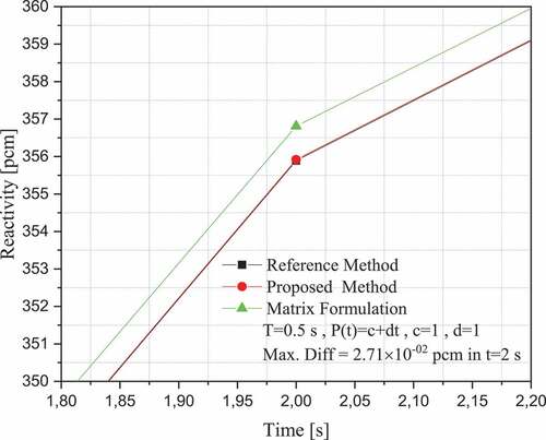
Figure 1 shows a part of the total reactivity curve in pcm to enable the appreciation of the difference between the Matrix Formulation methods [12] and the generalisation of the Bernoulli numbers, where the reference method is obtained by solving Equation (7)(7) $\rho (t)=\beta +\frac{\mathrm{\Lambda }}{P(t)}\frac{dP(t)}{dt}-\frac{P(0)}{P(t)}\sum _{i=1}^6{\beta }_i{e}^{-{\lambda }_{i}t}\text{break}-\frac{1}{P(t)}\sum _{i=1}^6\underset{0}{\overset{t}{\int }}{\lambda }_i{\beta }_i{e}^{-{\lambda }_i(t-t^{\prime })}P(t^{\prime })d{t}^{\prime }$(7) for a neutron population density form $P(t)=c+dt$ with a time step $T=0.5s$. It is possible to see that the matrix formulation method moves away from the solution given by the reference method.

Figure 1. Comparison of reactivity in pcm for a form of neutron population density $P(t)=c+dt$.

The cases presented so far include numerical experiments that meet the approximations given by Equations (28(28) $P^{(2k)}(t)=P(t){\left[\frac{P^{(2)}(t)}{P(t)}\right]}^k\equiv P(t)a^{2k};forallk\ge 0$(28) –30(30) $a^2=\left[\frac{P^{(2)}(t)}{P(t)}\right];forallt\ge 0$(30) ), where the matrix formulation method (FM) has very good approximations. In general terms, case studies 6–8 did not meet the conditions given by Equations (28(28) $P^{(2k)}(t)=P(t){\left[\frac{P^{(2)}(t)}{P(t)}\right]}^k\equiv P(t)a^{2k};forallk\ge 0$(28) –30(30) $a^2=\left[\frac{P^{(2)}(t)}{P(t)}\right];forallt\ge 0$(30) ).

Case study 6: In the following ninth numerical experiment, the power form of the neutron population density is changed to the form $P(t)=c+d{t}^3$. The results are shown in Table 10 for a time step $T=1s$for the calculation of the reactivity. It is observed that the method of generalisation of the Bernoulli numbers for this form of neutron density has a difference in the calculation of reactivity lower than the method of the derivatives (DM) [8] and the method of Matrix Formulation (MF) [12]. For the different values of d, the method of generalisation of Bernoulli numbers continues to have a better approximation. It can be observed from this numerical experiment how the proposed method has better approximations when compared to the derivative method (DM), although the two methods used the approximations given by Equations (28(28) $P^{(2k)}(t)=P(t){\left[\frac{P^{(2)}(t)}{P(t)}\right]}^k\equiv P(t)a^{2k};forallk\ge 0$(28) –30(30) $a^2=\left[\frac{P^{(2)}(t)}{P(t)}\right];forallt\ge 0$(30) ). In the proposed method represented by Equation (43)(43) $\begin{array}{rl}& \rho \left[n\right]={\rho }_{FIR}[n]+\frac{1}{P[n]}\\ & \left[\begin{array}{c}\left[\begin{array}{c}\left(P[n]+\frac{P^{(1)}[n]}{a}\right)\sum _{i=1}^6\frac{h_i[0]}{2(a+{\text{mr}\lambda }_i)}\left(\frac{z_{i,1}}{e^{z_{i,1}}-1}-1+\frac{z_{i,1}}{2}\right)\\ -\left(P[n]-\frac{P^{(1)}[n]}{a}\right)\sum _{i=1}^6\frac{h_i[0]}{2(a-{\lambda }_i)}\left(\frac{z_{i,2}}{e^{z_{i,2}}-1}-1+\frac{z_{i,2}}{2}\right)\end{array}\right]\\ -\left[\begin{array}{c}\left(P[0]+\frac{P^{(1)}[0]}{a}\right)\sum _{i=1}^6\frac{h_i[n]}{2(a+{\lambda }_i)}\left(\frac{z_{i,1}}{e^{z_{i,1}}-1}-1+\frac{z_{i,1}}{2}\right)\\ -\left(P[0]-\frac{P^{(1)}[0]}{a}\right)\sum _{i=1}^6\frac{h_i[n]}{2(a-{\lambda }_i)}\left(\frac{z_{i,2}}{e^{z_{i,2}}-1}-1+\frac{z_{i,2}}{2}\right)\end{array}\right]\end{array}\right]\end{array}$(43) , the dominant term for calculating reactivity for the case study is the first term given by ${\rho }_{FIR}[n]$, which has no restriction on the shape of the neutron density.

Table 10. Maximum difference in pcm for $P(t)=c+d{t}^3,\text{break}t=1000s$.

T [s]	c	d	DM	MF	BNGM	BNGM with eps
1	1	(0.0127) ^5/9	3.89×10^−03	1.42×10^−05	7.61×10^−11	7.61×10^−11
1	1	(0.0127) ^4/40	6.20×10^−02	9.57×10^−05	1.35×10^−09	1.35×10^−09
1	1	(0.0127) ^4/4	6.21×10^−01	4.38×10^−04	1.35×10^−08	1.35×10^−08

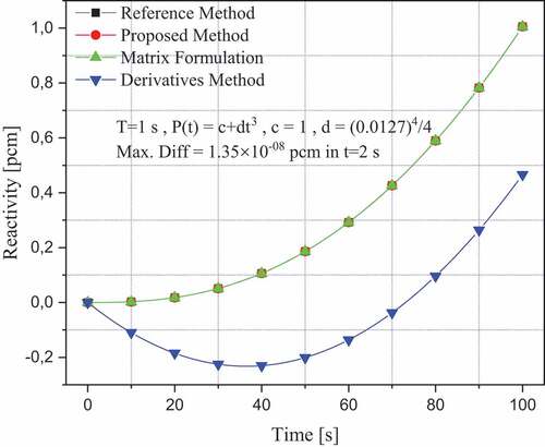
Figure 2 shows the reactivity curve in pcm for a form of neutron population density $P(t)=c+d{t}^3$ where the methods of Matrix Formulation [12], derivatives [8] and the generalisation of Bernoulli numbers are compared; The reference method is obtained by solving Equation (7)(7) $\rho (t)=\beta +\frac{\mathrm{\Lambda }}{P(t)}\frac{dP(t)}{dt}-\frac{P(0)}{P(t)}\sum _{i=1}^6{\beta }_i{e}^{-{\lambda }_{i}t}\text{break}-\frac{1}{P(t)}\sum _{i=1}^6\underset{0}{\overset{t}{\int }}{\lambda }_i{\beta }_i{e}^{-{\lambda }_i(t-t^{\prime })}P(t^{\prime })d{t}^{\prime }$(7) and the calculation in the simulation is done up to a final time of $t=100s$ with the purpose of better showing the shape of the reactivity curve. The low accuracy of the derivatives method is evidenced with respect to the good precision of the Matrix Formulation method and the excellent precision of the Bernoulli number generalisation method.

Figure 2. Comparison of reactivity in pcm for a form of neutron population density $P(t)=c+d{t}^3$.

Case study 7: The tenth and eleventh numerical experiments were dealt in this case. Tables 11 and 12 show the excellent accuracy of the method of generalisation of Bernoulli numbers for a hyperbolic form of neutron population density. It can be observed that the proposed method overwhelmingly exceeds the Matrix Formulation method, which until now had the best approximations in the calculation of reactivity.

Table 11. Maximum difference in pcm for $P(t)=c+cosh\text{break}(kt),t=180s$.

T [s]	c	k	MF	BNGM	BNGM with eps
0.1	0	$\pi /180$	1.35×10^−04	5.03×10^−12	1.72×10^−12
0.5	0	$\pi /180$	3.40×10^−03	1.87×10^−12	1.00×10^−12
1	0	$\pi /180$	1.34×10^−02	1.19×10^−12	1.12×10^−12
5	0	$\pi /180$	3.04×10^−01	1.04×10^−12	1.12×10^−12
0.1	100	$\pi /180$	1.43×10^−05	5.21×10^−13	2.43×10^−11
0.5	100	$\pi /180$	3.56×10^−04	3.77×10^−08	1.04×10^−08
1	100	$\pi /180$	1.40×10^−03	1.12×10^−07	1.12×10^−07
5	100	$\pi /180$	3.31×10^−02	1.75×10^−05	1.75×10^−05

Table 12. Maximum difference in pcm for $P(t)=c+sinh\text{break}(kt),t=10000s$.

T [s]	c	k	MF	BNGM	BNGM with eps
0.1	1	1.27×10^−03	7.56×10^−07	8.48×10^−10	8.28×10^−10
0.5	1	1.27×10^−03	1.88×10^−05	3.89×10^−07	3.89×10^−07
1	1	1.27×10^−03	7.47×10^−05	4.06×10^−06	4.05×10^−06
5	1	1.27×10^−03	1.70×10^−03	3.47×10^−04	3.47×10^−04
20	1	1.27×10^−03	1.02×10^−02	1.02×10^−02	1.02×10^−02
0.1	100	1.27×10^−3	2.33×10^−07	2.59×10^−12	6.93×10^−10
0.5	100	1.27×10^−3	5.81×10^−06	2.63×10^−10	3.38×10^−07
1	100	1.27×10^−3	2.31×10^−05	5.58×10^−09	3.76×10^−06
5	100	1.27×10^−3	5.33×10^−04	2.84×10^−06	3.35×10^−04
20	100	1.27×10^−3	6.68×10^−03	1.02×10^−03	1.02×10^−03

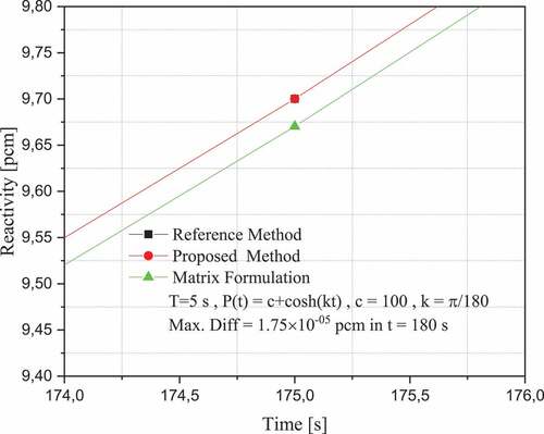
Figure 3 shows a comparison between the proposed method and the Matrix Formulation method for a neutron population density of the form $P(t)=c+cosh(kt)$ making use of eps. Because of the high precision of the proposed method and the Matrix Formulation method, the axis ranges are reduced to be able to observe the differences, so that a part of the total reactivity curve is shown. These results show the accuracy of the method using the generalisation of the Bernoulli numbers.

Figure 3. Comparison of reactivity in pcm for a form of neutron population density $P(t)=c+cosh(kt)$.

Case study 8: The last numerical experiment is presented in this case. Table 13 shows the difference in the calculation of the reactivity for a neutron population density of the form $P(t)=c+sin(kt)$. It is noted that the method of generalisation of Bernoulli numbers exceeds the Matrix Formulation method for all time steps.

Table 13. Maximum difference in pcm for $P(t)=c+sin\text{break}(kt),t=10s$.

T [s]	c	k	MF	BNGM	BNGM with eps
0.1	1	$\pi /10$	4.22×10^−02	1.14×10^−06	1.14×10^−06
0.5	1	$\pi /10$	1.05×10^0	5.94×10^−04	5.94×10^−04
1	1	$\pi /10$	4.15×10^0	7.62×10^−03	7.62×10^−03
5	1	$\pi /10$	8.55×10^1	1.46×10^0	1.46×10^0

The results presented in the studied cases 6–8, which do not meet the conditions (28–30), are of high precision using the proposed method, reaching several orders of magnitude when compared to the derivative methods (DM) and matrix formulation (MF).

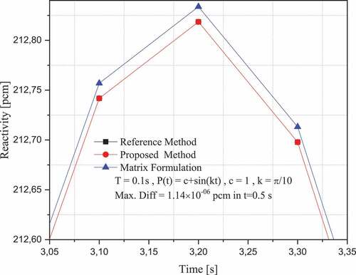
Figure 4 shows the reactivity curve for a neutron population density of the form $P(t)=c+sin(kt)$. Because of the high precision of the proposed method and the Matrix Formulation method with respect to the reference method, the axis ranges are narrowed, so that a part of the total reactivity curve is displayed. It is evident that the method of generalisation of Bernoulli numbers improves upon the reference method given by Equation (7)(7) $\rho (t)=\beta +\frac{\mathrm{\Lambda }}{P(t)}\frac{dP(t)}{dt}-\frac{P(0)}{P(t)}\sum _{i=1}^6{\beta }_i{e}^{-{\lambda }_{i}t}\text{break}-\frac{1}{P(t)}\sum _{i=1}^6\underset{0}{\overset{t}{\int }}{\lambda }_i{\beta }_i{e}^{-{\lambda }_i(t-t^{\prime })}P(t^{\prime })d{t}^{\prime }$(7) ; it is observed that the method of Matrix Formulation exceeds the reference method and the method of generalisation of the Bernoulli numbers due to the precision of the methods.

Figure 4. Comparison of reactivity in pcm for a form of neutron population density $P(t)=c+sin(kt)$.

5. Conclusions

In this work, a generalisation for the calculation of reactivity using the infinite numbers of Bernoulli was presented, this expression is simplified, firstly, by an approximation in the derivatives of the neutron density, secondly, using a Laurent’s series. The results presented are highly accurate in the calculation of reactivity when compared to those reported in the literature. It is evident from the different numerical experiments for different forms of neutron population density that the proposed method has a low computational cost since it is highly accurate regardless of the time step. Due to its high accuracy, it is recommended the proposed method to be implemented in a real-time digital reactivity meter.

Acknowledgments

The authors thank the research seed of Computational Physics, the research group in Applied Physics FIASUR, and the academic and financial support of the Universidad Surcolombiana.

Disclosure statement

No potential conflict of interest was reported by the authors.

References

- Weston MS. Nuclear reactor physics. 3rd ed. Weinheim (Germany): Wiley-VCH; 2018.
- Shimazu Y, Nakano Y, Tahara Y, et al. Development of a compact digital reactivity meter and reactor physics data processor. Nucl Technol. 1987;77:247–254.
- Ansari SA. Development of on-line reactivity meter for nuclear reactors. IEEE Trans Nucl Sci. 1991;38:946–952.
- Binney SE, Bakir AIM. Design and development of a personal computer based reactivity meter for a nuclear reactor. Nucl Technol. 1989;85:12–21.
- Hoogenboom JE. Van Der Sluijs AR. Neutron source strength determination for on-line reactivity measurements. Ann Nucl Energy. 1988;15:553–559.
- Tamura S. Signal fluctuation and neutron source in inverse kinetics method for reactivity measurement in the sub-critical domain. J Nucl Sci Technol. 2003;40:153–157.
- Kitano A, Itagaki M, Narita M. Memorial-index-based inverse kinetics method for continuous measurements of reactivity and source strength. J Nucl Sci Technol. 2000;37:53–59.
- Suescún DD, Martinez SA, Da Silva CF. Formulation for the calculation of reactivity without nuclear power history. J Nucl Sci Technol. 2007;44:1149–1155.
- Suescún DD, Martinez SA, Da Silva CF. Calculation of reactivity using a finite impulse response filter. Ann Nucl Energy. 2008;35:472–477.
- Hessam M, Vosoughi N. On-line reactivity calculation using Lagrange method. Ann Nucl Energy. 2013;62:463–467.
- Suescún DD, Rodriguez JA, Figueroa JH. Reactivity calculation using the Euler-Maclaurin formula. Ann Nucl Energy. 2013;53:104–108.
- Suescún DD, Cabrera CE, Lozano PJH. Matrix formulation for the calculation of nuclear reactivity. Ann Nucl Energy. 2018;116:137–142.
- Duderstadt JJ, Hamilton LJ. Nuclear reactor analysis. New York (NY): Wiley; 1976.
- Haykin S, Veen BV. Signal and system. New York (NY): Wiley; 1999.
- Kwok YK. Applied complex variable for scientist and engineers. 2nd ed. New York (NY): Cambridge; 2010.