Adjoint flux calculation of natural mode equation by time dependent neutron transport

ABSTRACT

The physical implication of the eigenfunction of the adjoint of the natural mode equation is studied. The eigenfunction at a phase space position is theoretically derived to be proportional to the amplitude of the neutron flux sufficiently long time after a source is placed at the position. Meanwhile, the time change rate and distribution of the neutron flux originated in the source must converge to those of the fundamental mode of the natural mode equation. Based on the proportional relation, the adjoint flux is calculated for a MOX- and UO₂-fueled lattice by a continuous-energy Monte Carlo time-dependent neutron transport calculation. The calculated distributions of the adjoint flux agree well with those of the iterated fission probability both in the prompt and delayed critical states.

KEYWORDS:

• Natural mode equation
• adjoint flux
• time-dependent neutron transport
• continuous-energy Monte Carlo
• iterated fission probability

1. Introduction

Neutron transport in a core is determined by the time-dependent neutron transport Equation [1]. When source neutrons are placed at a phase-space position defined by position r, energy E, and direction Ω (unit vector), various neutron flux modes arise and they propagate with time eigenvalue ω_mode. As time progresses, the relative amplitudes of the higher modes attenuate faster compared with that of the fundamental mode and, ultimately, the time change rate and spatial distribution of the neutron flux converge to those of the fundamental mode. After the convergence, the equation is reduced to the natural mode equation of which the eigenvalue is ω [2]. In a critical state, the fundamental mode equation of the natural mode is identical to that of the k-eigenvalue equation of which the eigenvalue is the effective multiplication factor k_eff.

The fundamental mode eigenvalue ω is a directly measurable parameter as the reciprocal of the reactor period and is traditionally used to assess the reactivity of a core in accordance with the inhour Equation [1]. The accurate estimation of ω is desirable for the safe design of the core in the case of reactivity insertion. In addition, the variation in ω due to the perturbations of the fission production and neutron annihilation operators has been derived by Endo [3] and Jinaphanh and Zoia [4]. The estimation error of ω could be a clue toward estimating the errors in the operators, such as those for nuclear data, nuclide density, and geometry. To relate the perturbation of the operators to the variation in ω, the flux φ_ω and the adjoint flux φ_ω^† are required, as in the application of perturbation theory to the k-eigenvalue equation. For the k-eigenvalue equation, continuous energy Monte Carlo (ceMC) calculation has already been performed for the flux φ_k and k_eff [5]. In 2009, Nauchi et al. firstly succeeded in calculating the adjoint flux φ_k^† of the k-eigenvalue Equation [6] and the adjoint-weighted kinetics parameters [7]. Furthermore, Kiedrowski et al. independently succeeded in calculating the kinetics parameters [8]. In their methods, the iterated fission probability (I_FP) was calculated explicitly or implicitly. I_FP at phase space position (r, E, Ω) represents the asymptotic core power in a generation in which the descendant neutrons originating in the source at (r, E, Ω) forms the fundamental mode neutron flux distribution of the k-eigenvalue equation. The proportional relation of I_FP and φ_k^† in the critical state was proven by Ussachof [9] and Hurwitz [10]. Nauchi has claimed that the theory can be extended to the non-critical states by clarifying the role of k_eff in the theory of Ussachoff [11]. Kiedrowski applied I_FP to perturbation theory to calculate the reactivity and its component [12]. Thanks to his work, I_FP has become one of the standard tools used to calculate the reactivity components and sensitivities through ceMC calculation (e.g. [13–15]).

Similar to I_FP in the k-eigenvalue equation, the adjoint flux of the natural mode equation, φ_ω^† is desired to be calculated in the ceMC manner. For this purpose, Terranova and Zoia developed the generalized iterated fission probability method (G-IFP) [16]. However, this method is not based on the natural behavior of neutrons and the implication of the adjoint flux deserves further investigations. Without considering the delayed neutron emission, Bell and Glasstone [17] theoretically derived that the adjoint flux φ_α^† is proportional to the number of neutron counts in a detector sufficiently long time after an original source neutron is placed at (r, E, Ω). The number of neutron counts is proportional to the amplitude of the neutron flux. Here, α is a special eigenvalue corresponding to ω where the delayed neutron emission is neglected.

Nauchi extended this theory to include the delayed neutron emission [18]. A comparison of the theory against G-IFP was successfully performed for a one–dimensional rod–type problem with two energy groups of reactor constants [19].

In this study, the extension of the theory to include the delayed neutron emission and the necessary conditions [18] are given and discussed in detail in Section 2. In order to perform the ceMC calculation of the adjoint flux φ_ω^† based on the extended theory, the time-dependent neutron transport calculation is required. For the prompt critical problem, the asymptotic time-dependent adjoint flux φ_α^†was calculated by the published version of MCNP-5 [5]. For the delayed critical problem, the adjoint flux φ_ω^† was calculated by employing the recently developed time-dependent neutron-transport-utilizing k-power iteration (TDPI) technique implemented in MCNP-5 [20]. To verify the calculated adjoint flux φ_α^†and φ_ω^†, comparisons with I_FP are presented in Section 3. Finally, the conclusion is given in Section 4.

2. Theory

2.1. Natural mode equation and perturbation theory

2.1.1. Natural mode equation

The time-dependent neutron flux Ψ(r, E, Ω, t) satisfies

(1) $\frac{1}{V}\frac{\mathrm{d}\psi }{\mathrm{d}t}=-\mathcal{L}\psi +{\mathcal{F}}_p\psi +{\sum }_j{\chi }_{d,j}{\lambda }_j{C}_j+{\mathrm{S}}_{ext}$(1)

Here, $\mathcal{L}$ is the net annihilation operator, and ${\mathcal{F}}_p$ is the prompt fission neutron emission operator of function f(r, E, Ω, t),

(2) $\mathcal{L}f=\mathbf{\Omega }\cdot \mathrm{\nabla }f+\left({\sum }_i{\sigma }_{tot,i}{N}_i\right)f-\int \int \mathrm{d}{\mathbf{\Omega }}_{in}\mathrm{d}{E}_{in}\left[{\sum }_i\left\{{\sigma }_{s,i}\left(r,E_{in}\to E,{\mathbf{\Omega }}_{in}\to \mathbf{\Omega }\right)N_i\right\}f\right]$(2)

(3) ${\mathcal{F}}_{p}f=\int \int \mathrm{d}{\mathbf{\Omega }}_{in}\mathrm{d}{E}_{in}\left[{\sum }_i\left\{{\chi }_{p,i}\left(E_{in}\to E\right){\nu }_{p,i}{\sigma }_{f,i}\left(r,E_{in}\right)N_i\right\}f\right]$(3)

Here, V, t, N, σ, ν, χ, λ, and C are the neutron speed, time, number density of nuclide, microscopic cross section, number of neutron emissions per fission, fission neutron emission spectrum, decay constant of precursor, and precursor density. The subscripts tot, s, f, i, j, in, p, and d denote total, scattering, fission, nuclide, precursor family, incident neutron, prompt neutron, and delayed neutron, respectively. S_ext refers an external neutron source. χ is normalized to unity when integrated over outgoing energy E_out and direction Ω_out,

(4) $1=\int \int \mathrm{d}{\mathrm{\Omega }}_{out}\mathrm{d}{E}_{out}{\chi }_{p,iord,j}$(4)

The time-dependent density of the precursors satisfies

(5) $\frac{\mathrm{d}{C}_j}{\mathrm{d}t}=-{\lambda }_j{C}_j+\int \int \mathrm{d}{\mathrm{\Omega }}_{in}\mathrm{d}{E}_{in}\left[{\sum }_i\left\{{\nu }_{d,ij}{\sigma }_{f,i}\left(\mathit{r},E_{in}\right)N_i\right\}\psi \right]$(5)

External neutron source S_ext is assumed to become to zero at time t = 0, and C_j and Ψ are positive at t = 0. At the time corresponding to the initial conditions, Ψ consists of the fundamental and higher modes [1]. However, the relative amplitude of the higher modes to that of the fundamental mode attenuates with time. As time progresses, Ψ converges to the product of the time-invariant spatial distribution of neutron flux φ_ω and the exponential change in the amplitude P_ω with t with time rate constant ω as follows.

(6) $\psi \to {\phi }_{\omega }{P}_{\omega }\left(t\right)={\phi }_{\omega }{P}_{\omega ,0}{e}^{\omega t}$(6)

In this case, the precursor density also varies exponentially with time with the same ω. Then, Equations (1)(1) $\frac{1}{V}\frac{\mathrm{d}\psi }{\mathrm{d}t}=-\mathcal{L}\psi +{\mathcal{F}}_p\psi +{\sum }_j{\chi }_{d,j}{\lambda }_j{C}_j+{\mathrm{S}}_{ext}$(1) and (5(5) $\frac{\mathrm{d}{C}_j}{\mathrm{d}t}=-{\lambda }_j{C}_j+\int \int \mathrm{d}{\mathrm{\Omega }}_{in}\mathrm{d}{E}_{in}\left[{\sum }_i\left\{{\nu }_{d,ij}{\sigma }_{f,i}\left(\mathit{r},E_{in}\right)N_i\right\}\psi \right]$(5) ) are reduced to

(7) $\frac{\omega }{V}{\phi }_{\omega }=-\mathcal{L}{\phi }_{\omega }+{\mathcal{F}}_p{\phi }_{\omega }+{\sum }_j\frac{{\lambda }_j}{\omega +{\lambda }_j}{\mathcal{F}}_{d,j}{\phi }_{\omega }$(7)

where ${\mathcal{F}}_{d,j}$ is the fission delayed neutron emission operator.

(8) ${\mathcal{F}}_{d,j}f=\int \int \mathrm{d}{\mathrm{\Omega }}_{in}\mathrm{d}{E}_{in}\left[{\sum }_i\left\{{\chi }_{d,j}\left(\mathrm{E}\right){\nu }_{d,ij}{\sigma }_{f,i}\left(\mathit{r},E\right)N_i\right\}f\right]$(8)

Equation (7)(7) $\frac{\omega }{V}{\phi }_{\omega }=-\mathcal{L}{\phi }_{\omega }+{\mathcal{F}}_p{\phi }_{\omega }+{\sum }_j\frac{{\lambda }_j}{\omega +{\lambda }_j}{\mathcal{F}}_{d,j}{\phi }_{\omega }$(7) is called the natural mode equation¹ [2], and ω is the eigenvalue of Equation (7)(7) $\frac{\omega }{V}{\phi }_{\omega }=-\mathcal{L}{\phi }_{\omega }+{\mathcal{F}}_p{\phi }_{\omega }+{\sum }_j\frac{{\lambda }_j}{\omega +{\lambda }_j}{\mathcal{F}}_{d,j}{\phi }_{\omega }$(7) .

2.1.2. Perturbation theory

There is the adjoint equation of Equation (7)(7) $\frac{\omega }{V}{\phi }_{\omega }=-\mathcal{L}{\phi }_{\omega }+{\mathcal{F}}_p{\phi }_{\omega }+{\sum }_j\frac{{\lambda }_j}{\omega +{\lambda }_j}{\mathcal{F}}_{d,j}{\phi }_{\omega }$(7) with the same eigenvalue ω and adjoint eigenfunction φ_ω^†,

(9) $\frac{\omega }{V}{{\phi }_{\omega }}^{†}=-{\mathcal{L}}^{†}{{\phi }_{\omega }}^{†}+{{\mathcal{F}}_p}^{†}{{\phi }_{\omega }}^{†}+{\sum }_j\frac{{\lambda }_j}{\omega +{\lambda }_j}{{\mathcal{F}}_{d,j}}^{†}{{\phi }_{\omega }}^{†}$(9)

The adjoint operators are the same as those used for the adjoint equations of the k-eigenvalue equation,

(10) ${\mathcal{L}}^{†}f=-\mathbf{\Omega }\cdot \mathrm{\nabla }f+\left({\sum }_i{\sigma }_{t,i}{N}_i\right)f-\int \int \mathrm{d}{\mathbf{\Omega }}_{out}\mathrm{d}{E}_{out}\left[{\sum }_i\left\{{\sigma }_{s,i}\left(\mathit{r},E\to E_{out},\mathbf{\Omega }\to {\mathbf{\Omega }}_{out}\right)N_i\right\}f\right]$(10)

(11) ${{\mathcal{F}}_p}^{†}f=\int \int \mathrm{d}{\mathrm{\Omega }}_{out}\mathrm{d}{E}_{out}\left[{\sum }_i\left\{{\chi }_{p,i}\left(\mathrm{E}\to E_{out}\right){\nu }_{p,i}{\sigma }_{f,i}\left(r,E\right)N_i\right\}f\right]$(11)

(12) ${{\mathcal{F}}_{d,j}}^{†}f=\int \int \mathrm{d}{\mathrm{\Omega }}_{out}\mathrm{d}{E}_{out}\left[{\sum }_i\left\{{\chi }_{d,j}\left(E_{out}\right){\nu }_{d,ij}{\sigma }_{f,i}\left(r,E\right)N_i\right\}f\right]$(12)

Considering the case in which the operators are perturbed by δ$\mathcal{L}$, δ${\mathcal{F}}_p$, and δ${\mathcal{F}}_{d,j}$,² such that ω and φ_ω change to ω’ and φ_ω’, respectively,

(13) $\frac{{\omega }^{\prime }}{V}{\phi }_{\omega }\prime =-\left(\mathcal{L}+\delta \mathcal{L}\right){{\phi }_{\omega }}^{\prime }+\left({\mathcal{F}}_p+\delta {\mathcal{F}}_p\right){{\phi }_{\omega }}^{\prime }+{\sum }_j\frac{{\lambda }_j}{{\omega }^{\prime }+{\lambda }_j}\left({\mathcal{F}}_{d,j}+\delta {\mathcal{F}}_{d,j}\right){{\phi }_{\omega }}^{\prime }$(13)

Multiplying Equation (13)(13) $\frac{{\omega }^{\prime }}{V}{\phi }_{\omega }\prime =-\left(\mathcal{L}+\delta \mathcal{L}\right){{\phi }_{\omega }}^{\prime }+\left({\mathcal{F}}_p+\delta {\mathcal{F}}_p\right){{\phi }_{\omega }}^{\prime }+{\sum }_j\frac{{\lambda }_j}{{\omega }^{\prime }+{\lambda }_j}\left({\mathcal{F}}_{d,j}+\delta {\mathcal{F}}_{d,j}\right){{\phi }_{\omega }}^{\prime }$(13) by φ_ω^† and Equation (9)(9) $\frac{\omega }{V}{{\phi }_{\omega }}^{†}=-{\mathcal{L}}^{†}{{\phi }_{\omega }}^{†}+{{\mathcal{F}}_p}^{†}{{\phi }_{\omega }}^{†}+{\sum }_j\frac{{\lambda }_j}{\omega +{\lambda }_j}{{\mathcal{F}}_{d,j}}^{†}{{\phi }_{\omega }}^{†}$(9) by φ_ω’ and then integrating the products over the entire phase space of energy, direction, and position (expressed as the angle brackets in Equation (14)(14) $\begin{array}{rl}& \left({\omega }^{\prime }-\omega \right){{\phi }_{\omega }}^{†}\frac{1}{V}{\phi }_{\omega }\prime =-{{\phi }_{\omega }}^{†}\delta \mathcal{L}{\phi }_{\omega }\prime +{{\phi }_{\omega }}^{†}\delta {\mathcal{F}}_p{\phi }_{\omega }\prime \\ & +{\sum }_j\frac{{\lambda }_j}{{\omega }^{\prime }+{\lambda }_j}{{\phi }_{\omega }}^{†}\left({\mathcal{F}}_{d,j}+\delta {\mathcal{F}}_{d,j}\right){{\phi }_{\omega }}^{\prime }\\ & -{\sum }_j\frac{{\lambda }_j}{\omega +{\lambda }_j}{{\phi }_{\omega }}^{†}{\mathcal{F}}_{d,j}{{\phi }_{\omega }}^{\prime }\end{array}$(14) ) yield the following differences in the integrated value [3,4]:

(14) $\begin{array}{rl}& \left({\omega }^{\prime }-\omega \right){{\phi }_{\omega }}^{†}\frac{1}{V}{\phi }_{\omega }\prime =-{{\phi }_{\omega }}^{†}\delta \mathcal{L}{\phi }_{\omega }\prime +{{\phi }_{\omega }}^{†}\delta {\mathcal{F}}_p{\phi }_{\omega }\prime \\ & +{\sum }_j\frac{{\lambda }_j}{{\omega }^{\prime }+{\lambda }_j}{{\phi }_{\omega }}^{†}\left({\mathcal{F}}_{d,j}+\delta {\mathcal{F}}_{d,j}\right){{\phi }_{\omega }}^{\prime }\\ & -{\sum }_j\frac{{\lambda }_j}{\omega +{\lambda }_j}{{\phi }_{\omega }}^{†}{\mathcal{F}}_{d,j}{{\phi }_{\omega }}^{\prime }\end{array}$(14)

This equation resembles the exact perturbation applied to the k-eigenvalue equation. With the adjoint flux φ_ω^†, the perturbation of the reaction rate is related to the perturbation of the eigenvalue. As ω is a measurable parameter, Endo claimed to use this relation to validate reactor physics calculations and nuclear data [3].

2.2. Implication of adjoint flux of natural mode equation

2.2.1. Adjoint natural mode equation

I(r, E, Ω) is defined as the expected amplitude of the neutron flux formed by a neutron and/or its descendant at a time t after the neutron is placed at phase space position (r, E, Ω). I(r, E, Ω) is time-invariant, and t is the time when the flux Ψ satisfies Equation (6)(6) $\psi \to {\phi }_{\omega }{P}_{\omega }\left(t\right)={\phi }_{\omega }{P}_{\omega ,0}{e}^{\omega t}$(6) . In Figure 1, neutron collision events on a track of infinitesimally short length dξ are schematically drawn. Here, the relocation of the precursor is neglected.

Figure 1. Schematic view of neutron collision on track.

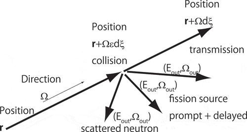
For a neutron at (r, E, Ω) and t = 0, I(r, E, Ω,) should be equal to the sum of the amplitudes of the neutron flux formed by the following components.

1. transmission neutrons at (r + Ω dξ,E,Ω) and time dξ/V,

2. scattered neutrons at (r+ Ωεdξ,E_out,Ω_out) and time εdξ/V,

3. prompt fission neutrons at (r+ Ωεdξ,E_out,Ω_out) and time εdξ/V,

4. delayed neutrons generated at (r+ Ωεdξ,E_out,Ω_out) and time τ when their precursors disintegrate by emission of them.

ε ranges from 0 to 1 to express the fact that the collision is occurred on the track. Here, the flight time of a neutron from (r, E, Ω) is explicitly considered with a speed of neutron, V, which is uniquely determined by E. As for the delayed neutron, the precursor is generated at time εdξ/V. However, the neutron emission is delayed and proceeds at time τ stochastically.

The expected number of neutrons per source for component 1) is

(15) $1-\mathrm{d}\xi \sum _{\mathrm{i}}{\sigma }_{t,i}{N}_i$(15)

The expected numbers of neutrons per source for components 2) and 3) are

(16) $\mathrm{d}\xi \sum _i{\sigma }_{s,i}\left(r+\mathrm{\Omega }\epsilon \mathrm{d}\xi ,E\to E_{out},\mathrm{\Omega }\to {\mathrm{\Omega }}_{out}\right)N_i$(16)

(17) $\mathrm{d}\xi \sum _i{\chi }_{p,i}\left(E\to E_{out}\right){\nu }_{p,i}{\sigma }_{f,i}\left(r+\mathrm{\Omega }\epsilon \mathrm{d}\xi ,E\right)N_i$(17)

respectively. The expected number of generated delayed neutron precursors at time εdξ/V is

(18) $\mathrm{d}\xi \sum _{ij}{\nu }_{d,ij}{\sigma }_{f,i}\left(r+\mathrm{\Omega }\epsilon \mathrm{d}\xi ,E\right)N_i$(18)

The expected number of delayed neutron emissions in time region τ to τ+ dτ by precursors made at r + Ω εdξ and time εdξ/V is

(19) $\mathrm{d}\xi \sum _{ij}{\chi }_{d,j}\left(E_{out}\right){\nu }_{d,ij}{\sigma }_{f,i}\left(r+\mathrm{\Omega }\epsilon \mathrm{d}\xi ,E\right)N_{i}exp\left(-{\lambda }_j\left(\tau -\frac{\epsilon \mathrm{d}\xi }{V}\right)\right){\lambda }_j\mathrm{d}\tau$(19)

Because I is the expected amplitude of flux at some time t, the difference in the emission time of neutrons of each component should be considered in the balance equation of the amplitude at time t. At time t, the amplitude of the neutron flux varies in accordance with Equation (6)(6) $\psi \to {\phi }_{\omega }{P}_{\omega }\left(t\right)={\phi }_{\omega }{P}_{\omega ,0}{e}^{\omega t}$(6) . Accordingly, the influence of time difference Δt can be corrected by multiplying I by exp(-ω ∙ Δt).

(20) $\begin{array}{rl}& I\left(\mathit{r},E,\mathbf{\Omega }\right)=\left(1-\mathrm{d}\xi \sum _i{\sigma }_{t,i}{N}_i\right)\\ & exp\left(-\omega \frac{\mathrm{d}\xi }{V}\right)I\left(\mathit{r}+\mathrm{\Omega }\mathrm{d}\xi ,E,\mathrm{\Omega }\right)\\ & +\int \int \mathrm{d}{\mathrm{\Omega }}_{out}\mathrm{d}{E}_{out}\left[\mathrm{d}\xi \sum _i\left\{\left\{{\sigma }_{s,i}\left(\mathit{r}\right.\right.\right.\right.\\ & \left.+\mathrm{\Omega }\epsilon \mathrm{d}\xi ,E\to E_{out},\mathrm{\Omega }\to {\mathrm{\Omega }}_{out}\right)\\ & \left.\left.+{\chi }_{p,i}\left(E\to E_{out}\right){\nu }_{p,i}{\sigma }_{f,i}\left(\mathit{r}+\mathrm{\Omega }\epsilon \mathrm{d}\xi ,E\right)\right\}{N}_i\right\}\\ & \left.exp\left(-\omega \epsilon \frac{\mathrm{d}\xi }{V}\right)I\left(\mathit{r}+\mathrm{\Omega }\epsilon \mathrm{d}\xi ,E_{out},{\mathrm{\Omega }}_{out}\right)\right]\\ & +\int \int \mathrm{d}{\mathrm{\Omega }}_{out}\mathrm{d}{E}_{out}\left[\underset{\epsilon \frac{\mathrm{d}\xi }{V}}{\overset{t}{\int }}\mathrm{d}\tau \left\{\mathrm{d}\xi \sum _{ij}\left\{{\lambda }_j{\chi }_{d,j}\left(E_{out}\right){\nu }_{d,ij}\right.\right.\right.\\ & {\sigma }_{f,i}\left(\mathit{r}+\mathrm{\Omega }\epsilon \mathrm{d}\xi ,E\right)N_i\left.\cdot exp\left(-{\lambda }_j\left(\tau -\frac{\epsilon \mathrm{d}\xi }{V}\right)\right)\right\}\\ & \left.exp\left(-\omega \left(\tau -\epsilon \frac{\mathrm{d}\xi }{V}\right)\right)\right\}\left.I\left(\mathit{r}+\mathrm{\Omega }\epsilon \mathrm{d}\xi ,E_{out},{\mathrm{\Omega }}_{out}\right)\right]\end{array}$(20)

In this study, the time delay effect is explicitly considered to take the delayed neutron into account. This time correction is analogous to the role of k_eff in the balance equation of I_FP(r, E, Ω) as clarified in [11]. In the framework of the k-power iteration, the fission neutron emission is treated as the event in the next cycle, whereas the transmission and the scattering are done as those in the current cycle. To achieve a balance of the descendant neutrons of the incident and the fission neutrons with I_FP(r, E, Ω), I_FP(r, E, Ω)/k_eff is used for the fission neutron source [11].

Subtracting I(r, E, Ω) from both sides of Equation (20)(20) $\begin{array}{rl}& I\left(\mathit{r},E,\mathbf{\Omega }\right)=\left(1-\mathrm{d}\xi \sum _i{\sigma }_{t,i}{N}_i\right)\\ & exp\left(-\omega \frac{\mathrm{d}\xi }{V}\right)I\left(\mathit{r}+\mathrm{\Omega }\mathrm{d}\xi ,E,\mathrm{\Omega }\right)\\ & +\int \int \mathrm{d}{\mathrm{\Omega }}_{out}\mathrm{d}{E}_{out}\left[\mathrm{d}\xi \sum _i\left\{\left\{{\sigma }_{s,i}\left(\mathit{r}\right.\right.\right.\right.\\ & \left.+\mathrm{\Omega }\epsilon \mathrm{d}\xi ,E\to E_{out},\mathrm{\Omega }\to {\mathrm{\Omega }}_{out}\right)\\ & \left.\left.+{\chi }_{p,i}\left(E\to E_{out}\right){\nu }_{p,i}{\sigma }_{f,i}\left(\mathit{r}+\mathrm{\Omega }\epsilon \mathrm{d}\xi ,E\right)\right\}{N}_i\right\}\\ & \left.exp\left(-\omega \epsilon \frac{\mathrm{d}\xi }{V}\right)I\left(\mathit{r}+\mathrm{\Omega }\epsilon \mathrm{d}\xi ,E_{out},{\mathrm{\Omega }}_{out}\right)\right]\\ & +\int \int \mathrm{d}{\mathrm{\Omega }}_{out}\mathrm{d}{E}_{out}\left[\underset{\epsilon \frac{\mathrm{d}\xi }{V}}{\overset{t}{\int }}\mathrm{d}\tau \left\{\mathrm{d}\xi \sum _{ij}\left\{{\lambda }_j{\chi }_{d,j}\left(E_{out}\right){\nu }_{d,ij}\right.\right.\right.\\ & {\sigma }_{f,i}\left(\mathit{r}+\mathrm{\Omega }\epsilon \mathrm{d}\xi ,E\right)N_i\left.\cdot exp\left(-{\lambda }_j\left(\tau -\frac{\epsilon \mathrm{d}\xi }{V}\right)\right)\right\}\\ & \left.exp\left(-\omega \left(\tau -\epsilon \frac{\mathrm{d}\xi }{V}\right)\right)\right\}\left.I\left(\mathit{r}+\mathrm{\Omega }\epsilon \mathrm{d}\xi ,E_{out},{\mathrm{\Omega }}_{out}\right)\right]\end{array}$(20) and taking the first-order Taylor expansion for the exponential terms concerning the time delays on the track,

(21) $\begin{array}{l}0=-Ir,E,\Omega +\left(1-\text{d}\xi {\displaystyle \sum _i{\sigma }_{t,i}}{N}_i\right)\left(1-\omega \frac{\text{d}\xi }{V}\right)\\ I\left(r+\Omega \text{d}\xi ,E,\Omega \right)+\text{d}\xi {\displaystyle \int {\displaystyle \int \text{d}}}{\Omega }_{out}\text{d}{E}_{out}\\ [{\displaystyle \sum _i\{\{{\sigma }_{s,i}\left(r+\Omega \epsilon \text{d}\xi ,E\to E_{out},\Omega \to {\Omega }_{out}\right)}\\ +{\chi }_{p,i}\left(E\to E_{out}\right){\nu }_{p,i}{\sigma }_{f,i}\left(r+\Omega \epsilon \text{d}\xi ,E\right)\}{N}_i\}\\ \left(1-\omega \epsilon \frac{\text{d}\xi }{V}\right)I(r+\Omega \epsilon \text{d}\xi ,E_{out},{\Omega }_{out})]+\text{d}\xi {\displaystyle \int {\displaystyle \int \text{d}}}{\Omega }_{out}\text{d}{E}_{out}\\ [{\displaystyle \underset{\epsilon \frac{\text{d}\xi }{V}}{\overset{t}{\int }}\text{d}\tau {\displaystyle \sum _{ij}\{{\lambda }_j{\chi }_{d,j}\left(E_{out}\right){\nu }_{d,ij}{\sigma }_{f,i}\left(r+\Omega \epsilon \text{d}\xi ,E\right)N_i}}\\ \cdot exp\left(-\left(\omega +{\lambda }_j\right)\left(\tau -\frac{\epsilon \text{d}\xi }{V}\right)\right)\}I\left(r+\Omega \epsilon \text{d}\xi ,E_{out},{\Omega }_{out}\right)]\end{array}$(21)

is given. Here the exponential term in the delayed neutron emission is transformed. Then, the quadratic terms of dξ can be neglected, and the Taylor expansion of I is taken for the second term of the right-hand side of Equation (21)(21) $\begin{array}{l}0=-Ir,E,\Omega +\left(1-\text{d}\xi {\displaystyle \sum _i{\sigma }_{t,i}}{N}_i\right)\left(1-\omega \frac{\text{d}\xi }{V}\right)\\ I\left(r+\Omega \text{d}\xi ,E,\Omega \right)+\text{d}\xi {\displaystyle \int {\displaystyle \int \text{d}}}{\Omega }_{out}\text{d}{E}_{out}\\ [{\displaystyle \sum _i\{\{{\sigma }_{s,i}\left(r+\Omega \epsilon \text{d}\xi ,E\to E_{out},\Omega \to {\Omega }_{out}\right)}\\ +{\chi }_{p,i}\left(E\to E_{out}\right){\nu }_{p,i}{\sigma }_{f,i}\left(r+\Omega \epsilon \text{d}\xi ,E\right)\}{N}_i\}\\ \left(1-\omega \epsilon \frac{\text{d}\xi }{V}\right)I(r+\Omega \epsilon \text{d}\xi ,E_{out},{\Omega }_{out})]+\text{d}\xi {\displaystyle \int {\displaystyle \int \text{d}}}{\Omega }_{out}\text{d}{E}_{out}\\ [{\displaystyle \underset{\epsilon \frac{\text{d}\xi }{V}}{\overset{t}{\int }}\text{d}\tau {\displaystyle \sum _{ij}\{{\lambda }_j{\chi }_{d,j}\left(E_{out}\right){\nu }_{d,ij}{\sigma }_{f,i}\left(r+\Omega \epsilon \text{d}\xi ,E\right)N_i}}\\ \cdot exp\left(-\left(\omega +{\lambda }_j\right)\left(\tau -\frac{\epsilon \text{d}\xi }{V}\right)\right)\}I\left(r+\Omega \epsilon \text{d}\xi ,E_{out},{\Omega }_{out}\right)]\end{array}$(21) . Integration of the delayed neutron emission term to τ is also performed.

(22) $\begin{array}{rl}& 0=\mathrm{d}\xi \mathrm{\Omega }\frac{d}{\mathrm{d}\xi }I\left(\mathit{r},E,\mathrm{\Omega }\right)-\mathrm{d}\xi \left(\sum _i{\sigma }_{t,i}{N}_i+\frac{\omega }{V}\right)I\left(\mathit{r}+\mathrm{\Omega }\mathrm{d}\xi ,E,\mathrm{\Omega }\right)\\ & +\mathrm{d}\xi \int \int \mathrm{d}{\mathrm{\Omega }}_{out}\mathrm{d}{E}_{out}\left[\sum _i\left\{\left\{{\sigma }_{s,i}\left(\mathit{r}+\mathrm{\Omega }\epsilon \mathrm{d}\xi ,E\to E_{out},\mathrm{\Omega }\to {\mathrm{\Omega }}_{out}\right)\right.\right.\right.\\ & \left.\left.+{\chi }_{p,i}\left(E\to E_{out}\right){\nu }_{p,i}{\sigma }_{f,i}\left(\mathit{r}+\mathrm{\Omega }\epsilon \mathrm{d}\xi ,E\right)\right\}{N}_i\right\}\left(1-\omega \epsilon \frac{\mathrm{d}\xi }{V}\right)\\ & \left.I\left(\mathit{r}+\mathrm{\Omega }\epsilon \mathrm{d}\xi ,E_{out},{\mathrm{\Omega }}_{out}\right)\right]+\mathrm{d}\xi \int \int \mathrm{d}{\mathrm{\Omega }}_{out}\mathrm{d}{E}_{out}\\ & \left[\sum _{ij}\left\{\frac{{\lambda }_j}{\omega +{\lambda }_j}{\chi }_{d,j}\left(E_{out}\right){\nu }_{d,ij}{\sigma }_{f,i}\left(\mathit{r}+\mathrm{\Omega }\epsilon \mathrm{d}\xi ,E\right)N_i\right.\right.\\ & \left.\left.\cdot \left(1-exp\left(-\left(\omega +{\lambda }_j\right)\left(t-\frac{\epsilon \mathrm{d}\xi }{V}\right)\right)\right)\right\}I\left(\mathit{r}+\mathrm{\Omega }\epsilon \mathrm{d}\xi ,E_{out},{\mathrm{\Omega }}_{out}\right)\right]\end{array}$(22)

The first term of the right-hand side of Equation (22)(22) $\begin{array}{rl}& 0=\mathrm{d}\xi \mathrm{\Omega }\frac{d}{\mathrm{d}\xi }I\left(\mathit{r},E,\mathrm{\Omega }\right)-\mathrm{d}\xi \left(\sum _i{\sigma }_{t,i}{N}_i+\frac{\omega }{V}\right)I\left(\mathit{r}+\mathrm{\Omega }\mathrm{d}\xi ,E,\mathrm{\Omega }\right)\\ & +\mathrm{d}\xi \int \int \mathrm{d}{\mathrm{\Omega }}_{out}\mathrm{d}{E}_{out}\left[\sum _i\left\{\left\{{\sigma }_{s,i}\left(\mathit{r}+\mathrm{\Omega }\epsilon \mathrm{d}\xi ,E\to E_{out},\mathrm{\Omega }\to {\mathrm{\Omega }}_{out}\right)\right.\right.\right.\\ & \left.\left.+{\chi }_{p,i}\left(E\to E_{out}\right){\nu }_{p,i}{\sigma }_{f,i}\left(\mathit{r}+\mathrm{\Omega }\epsilon \mathrm{d}\xi ,E\right)\right\}{N}_i\right\}\left(1-\omega \epsilon \frac{\mathrm{d}\xi }{V}\right)\\ & \left.I\left(\mathit{r}+\mathrm{\Omega }\epsilon \mathrm{d}\xi ,E_{out},{\mathrm{\Omega }}_{out}\right)\right]+\mathrm{d}\xi \int \int \mathrm{d}{\mathrm{\Omega }}_{out}\mathrm{d}{E}_{out}\\ & \left[\sum _{ij}\left\{\frac{{\lambda }_j}{\omega +{\lambda }_j}{\chi }_{d,j}\left(E_{out}\right){\nu }_{d,ij}{\sigma }_{f,i}\left(\mathit{r}+\mathrm{\Omega }\epsilon \mathrm{d}\xi ,E\right)N_i\right.\right.\\ & \left.\left.\cdot \left(1-exp\left(-\left(\omega +{\lambda }_j\right)\left(t-\frac{\epsilon \mathrm{d}\xi }{V}\right)\right)\right)\right\}I\left(\mathit{r}+\mathrm{\Omega }\epsilon \mathrm{d}\xi ,E_{out},{\mathrm{\Omega }}_{out}\right)\right]\end{array}$(22) can be expressed with the inner product of dξΩ and the gradient of I. Then, Equation (22)(22) $\begin{array}{rl}& 0=\mathrm{d}\xi \mathrm{\Omega }\frac{d}{\mathrm{d}\xi }I\left(\mathit{r},E,\mathrm{\Omega }\right)-\mathrm{d}\xi \left(\sum _i{\sigma }_{t,i}{N}_i+\frac{\omega }{V}\right)I\left(\mathit{r}+\mathrm{\Omega }\mathrm{d}\xi ,E,\mathrm{\Omega }\right)\\ & +\mathrm{d}\xi \int \int \mathrm{d}{\mathrm{\Omega }}_{out}\mathrm{d}{E}_{out}\left[\sum _i\left\{\left\{{\sigma }_{s,i}\left(\mathit{r}+\mathrm{\Omega }\epsilon \mathrm{d}\xi ,E\to E_{out},\mathrm{\Omega }\to {\mathrm{\Omega }}_{out}\right)\right.\right.\right.\\ & \left.\left.+{\chi }_{p,i}\left(E\to E_{out}\right){\nu }_{p,i}{\sigma }_{f,i}\left(\mathit{r}+\mathrm{\Omega }\epsilon \mathrm{d}\xi ,E\right)\right\}{N}_i\right\}\left(1-\omega \epsilon \frac{\mathrm{d}\xi }{V}\right)\\ & \left.I\left(\mathit{r}+\mathrm{\Omega }\epsilon \mathrm{d}\xi ,E_{out},{\mathrm{\Omega }}_{out}\right)\right]+\mathrm{d}\xi \int \int \mathrm{d}{\mathrm{\Omega }}_{out}\mathrm{d}{E}_{out}\\ & \left[\sum _{ij}\left\{\frac{{\lambda }_j}{\omega +{\lambda }_j}{\chi }_{d,j}\left(E_{out}\right){\nu }_{d,ij}{\sigma }_{f,i}\left(\mathit{r}+\mathrm{\Omega }\epsilon \mathrm{d}\xi ,E\right)N_i\right.\right.\\ & \left.\left.\cdot \left(1-exp\left(-\left(\omega +{\lambda }_j\right)\left(t-\frac{\epsilon \mathrm{d}\xi }{V}\right)\right)\right)\right\}I\left(\mathit{r}+\mathrm{\Omega }\epsilon \mathrm{d}\xi ,E_{out},{\mathrm{\Omega }}_{out}\right)\right]\end{array}$(22) is divided by dξ and the limit as dξ→0 is taken,

(23) $\begin{array}{rl}& 0=\mathrm{\Omega }\cdot \mathrm{\nabla }I\left(\mathit{r},E,\mathrm{\Omega }\right)-\left(\sum _i{\sigma }_{t,i}{N}_i+\frac{\omega }{V}\right)I\left(\mathit{r},E,\mathrm{\Omega }\right)\\ & +\int \int \mathrm{d}{\mathrm{\Omega }}_{out}\mathrm{d}{E}_{out}\left[\sum _i\left\{\left\{{\sigma }_{s,i}\left(\mathit{r},E\to E_{out},\mathrm{\Omega }\to {\mathrm{\Omega }}_{out}\right)\right.\right.\right.\\ & \left.\left.\left.+{\chi }_{p,i}\left(E\to E_{out}\right){\nu }_{p,i}{\sigma }_{f,i}\left(\mathit{r},E\right)\right\}{N}_i\right\}I\left(\mathit{r},E_{out},{\mathrm{\Omega }}_{out}\right)\right]\\ & +\int \int \mathrm{d}{\mathrm{\Omega }}_{out}\mathrm{d}{E}_{out}\left[\sum _{ij}\left\{\frac{{\lambda }_j}{\omega +{\lambda }_j}{\chi }_{d,j}\left(E_{out}\right){\nu }_{d,ij}{\sigma }_{f,i}\left(\mathit{r},E\right)N_i\right.\right.\\ & \left.\cdot \left.\left(1-exp\left(-\left(\omega +{\lambda }_j\right)t\right)\right)\right\}I\left(\mathit{r},E_{out},{\mathrm{\Omega }}_{out}\right)\right]\end{array}$(23)

Generally [1], real eigenvalue ω of the fundamental mode satisfies

(24) $\omega >-\mathrm{m}\mathrm{i}\mathrm{n}\left\{{\lambda }_j\right\}$(24)

Accordingly, when the flux originating in a neutron at (r, E, Ω) converges to the fundamental mode (Equation (6)(6) $\psi \to {\phi }_{\omega }{P}_{\omega }\left(t\right)={\phi }_{\omega }{P}_{\omega ,0}{e}^{\omega t}$(6) is satisfied) and t is large enough to satisfy

(25) $exp\left(-\left(\omega +{\lambda }_j\right)t\right)\to 0$(25)

the following equation is given.

(26) $\begin{array}{rl}& \frac{\omega }{V}I=\mathrm{\Omega }\cdot \mathrm{\nabla }I-\sum _i{\sigma }_{t,i}{N}_{i}I\\ & +\int {\int }^{\mathrm{d}}{\mathrm{\Omega }}_{out}\mathrm{d}{E}_{out}\left[\sum _i\left\{\left\{{\sigma }_{s,i}\left(r,E\to E_{out},\mathrm{\Omega }\to {\mathrm{\Omega }}_{out}\right)\right.\right.\right.\\ & \left.\left.\left.+{\chi }_{p,i}\left(E\to E_{out}\right){\nu }_{p,i}{\sigma }_{f,i}\left(r,E\right)\right\}{N}_i\right\}I\left(r,E_{out},{\mathrm{\Omega }}_{out}\right)\right]\\ & +\sum _{ij}\frac{{\lambda }_j}{\omega +{\lambda }_j}\int {\int }^{\mathrm{d}}{\mathrm{\Omega }}_{out}\mathrm{d}{E}_{out}\left[{\chi }_{d,j}\left(E_{out}\right){\nu }_{d,ij}{\sigma }_{f,i}\left(r,E\right)\right.\\ & \left.N_{i}I\left(r,E_{out},{\mathrm{\Omega }}_{out}\right)\right]\end{array}$(26)

This balance equation of I is identical to that of φ_ω^† (Equation (9)(9) $\frac{\omega }{V}{{\phi }_{\omega }}^{†}=-{\mathcal{L}}^{†}{{\phi }_{\omega }}^{†}+{{\mathcal{F}}_p}^{†}{{\phi }_{\omega }}^{†}+{\sum }_j\frac{{\lambda }_j}{\omega +{\lambda }_j}{{\mathcal{F}}_{d,j}}^{†}{{\phi }_{\omega }}^{†}$(9) ). Thus, it is concluded that the implication of the adjoint flux of the natural mode equation, φ_ω^†, is the quantity proportional to the amplitude of the neutron flux at some time t after a source is placed at (r, E, Ω), provided that t is sufficiently long such that Equations. (6)(6) $\psi \to {\phi }_{\omega }{P}_{\omega }\left(t\right)={\phi }_{\omega }{P}_{\omega ,0}{e}^{\omega t}$(6) and (25(25) $exp\left(-\left(\omega +{\lambda }_j\right)t\right)\to 0$(25) ) are satisfied [18].

2.2.2. Adjoint natural mode equation without delayed neutron

Even in the case in which the delayed neutron does not exist, the amplitude eventually varies exponentially with time with a constant α_p. I_α is defined as the amplitude of the neutron flux at some time when the neutron flux is dominated by the fundamental mode in a system without a delayed neutron. Bell and Glasstone derived the balance equation neglecting the delayed neutron emission and the time-delay effect shown in Equation (20)(20) $\begin{array}{rl}& I\left(\mathit{r},E,\mathbf{\Omega }\right)=\left(1-\mathrm{d}\xi \sum _i{\sigma }_{t,i}{N}_i\right)\\ & exp\left(-\omega \frac{\mathrm{d}\xi }{V}\right)I\left(\mathit{r}+\mathrm{\Omega }\mathrm{d}\xi ,E,\mathrm{\Omega }\right)\\ & +\int \int \mathrm{d}{\mathrm{\Omega }}_{out}\mathrm{d}{E}_{out}\left[\mathrm{d}\xi \sum _i\left\{\left\{{\sigma }_{s,i}\left(\mathit{r}\right.\right.\right.\right.\\ & \left.+\mathrm{\Omega }\epsilon \mathrm{d}\xi ,E\to E_{out},\mathrm{\Omega }\to {\mathrm{\Omega }}_{out}\right)\\ & \left.\left.+{\chi }_{p,i}\left(E\to E_{out}\right){\nu }_{p,i}{\sigma }_{f,i}\left(\mathit{r}+\mathrm{\Omega }\epsilon \mathrm{d}\xi ,E\right)\right\}{N}_i\right\}\\ & \left.exp\left(-\omega \epsilon \frac{\mathrm{d}\xi }{V}\right)I\left(\mathit{r}+\mathrm{\Omega }\epsilon \mathrm{d}\xi ,E_{out},{\mathrm{\Omega }}_{out}\right)\right]\\ & +\int \int \mathrm{d}{\mathrm{\Omega }}_{out}\mathrm{d}{E}_{out}\left[\underset{\epsilon \frac{\mathrm{d}\xi }{V}}{\overset{t}{\int }}\mathrm{d}\tau \left\{\mathrm{d}\xi \sum _{ij}\left\{{\lambda }_j{\chi }_{d,j}\left(E_{out}\right){\nu }_{d,ij}\right.\right.\right.\\ & {\sigma }_{f,i}\left(\mathit{r}+\mathrm{\Omega }\epsilon \mathrm{d}\xi ,E\right)N_i\left.\cdot exp\left(-{\lambda }_j\left(\tau -\frac{\epsilon \mathrm{d}\xi }{V}\right)\right)\right\}\\ & \left.exp\left(-\omega \left(\tau -\epsilon \frac{\mathrm{d}\xi }{V}\right)\right)\right\}\left.I\left(\mathit{r}+\mathrm{\Omega }\epsilon \mathrm{d}\xi ,E_{out},{\mathrm{\Omega }}_{out}\right)\right]\end{array}$(20) [17].

(27) $\begin{array}{rl}& I_{\alpha }\left(\mathit{r},E,\mathbf{\Omega }\right)=\left(1-\mathrm{d}\xi \sum _i{\sigma }_{t,i}{N}_i\right)\\ & I_{\alpha }\left(\mathit{r}+\mathrm{\Omega }\mathrm{d}\xi ,E,\mathrm{\Omega }\right)+\int \int \mathrm{d}{\mathrm{\Omega }}_{out}\mathrm{d}{E}_{out}\\ & \left[\mathrm{d}\xi \sum _i\left\{\left\{{\sigma }_{s,i}\left(\mathit{r}+\mathrm{\Omega }\epsilon \mathrm{d}\xi ,E\to E_{out},\mathrm{\Omega }\to {\mathrm{\Omega }}_{out}\right)\right.\right.\right.\\ & \left.+{\chi }_{p,i}\left(E\to E_{out}\right){\nu }_{p,i}{\sigma }_{f,i}\left(\mathit{r}+\mathrm{\Omega }\epsilon \mathrm{d}\xi ,E\right)\right\}\left.N_i\right\}\\ & \left.I_{\alpha }\left(\mathit{r}+\mathrm{\Omega }\epsilon \mathrm{d}\xi ,E_{out},{\mathrm{\Omega }}_{out}\right)\right]\end{array}$(27)

As the same procedure is used for Equations (20)(20) $\begin{array}{rl}& I\left(\mathit{r},E,\mathbf{\Omega }\right)=\left(1-\mathrm{d}\xi \sum _i{\sigma }_{t,i}{N}_i\right)\\ & exp\left(-\omega \frac{\mathrm{d}\xi }{V}\right)I\left(\mathit{r}+\mathrm{\Omega }\mathrm{d}\xi ,E,\mathrm{\Omega }\right)\\ & +\int \int \mathrm{d}{\mathrm{\Omega }}_{out}\mathrm{d}{E}_{out}\left[\mathrm{d}\xi \sum _i\left\{\left\{{\sigma }_{s,i}\left(\mathit{r}\right.\right.\right.\right.\\ & \left.+\mathrm{\Omega }\epsilon \mathrm{d}\xi ,E\to E_{out},\mathrm{\Omega }\to {\mathrm{\Omega }}_{out}\right)\\ & \left.\left.+{\chi }_{p,i}\left(E\to E_{out}\right){\nu }_{p,i}{\sigma }_{f,i}\left(\mathit{r}+\mathrm{\Omega }\epsilon \mathrm{d}\xi ,E\right)\right\}{N}_i\right\}\\ & \left.exp\left(-\omega \epsilon \frac{\mathrm{d}\xi }{V}\right)I\left(\mathit{r}+\mathrm{\Omega }\epsilon \mathrm{d}\xi ,E_{out},{\mathrm{\Omega }}_{out}\right)\right]\\ & +\int \int \mathrm{d}{\mathrm{\Omega }}_{out}\mathrm{d}{E}_{out}\left[\underset{\epsilon \frac{\mathrm{d}\xi }{V}}{\overset{t}{\int }}\mathrm{d}\tau \left\{\mathrm{d}\xi \sum _{ij}\left\{{\lambda }_j{\chi }_{d,j}\left(E_{out}\right){\nu }_{d,ij}\right.\right.\right.\\ & {\sigma }_{f,i}\left(\mathit{r}+\mathrm{\Omega }\epsilon \mathrm{d}\xi ,E\right)N_i\left.\cdot exp\left(-{\lambda }_j\left(\tau -\frac{\epsilon \mathrm{d}\xi }{V}\right)\right)\right\}\\ & \left.exp\left(-\omega \left(\tau -\epsilon \frac{\mathrm{d}\xi }{V}\right)\right)\right\}\left.I\left(\mathit{r}+\mathrm{\Omega }\epsilon \mathrm{d}\xi ,E_{out},{\mathrm{\Omega }}_{out}\right)\right]\end{array}$(20) –(20) $\begin{array}{rl}& I\left(\mathit{r},E,\mathbf{\Omega }\right)=\left(1-\mathrm{d}\xi \sum _i{\sigma }_{t,i}{N}_i\right)\\ & exp\left(-\omega \frac{\mathrm{d}\xi }{V}\right)I\left(\mathit{r}+\mathrm{\Omega }\mathrm{d}\xi ,E,\mathrm{\Omega }\right)\\ & +\int \int \mathrm{d}{\mathrm{\Omega }}_{out}\mathrm{d}{E}_{out}\left[\mathrm{d}\xi \sum _i\left\{\left\{{\sigma }_{s,i}\left(\mathit{r}\right.\right.\right.\right.\\ & \left.+\mathrm{\Omega }\epsilon \mathrm{d}\xi ,E\to E_{out},\mathrm{\Omega }\to {\mathrm{\Omega }}_{out}\right)\\ & \left.\left.+{\chi }_{p,i}\left(E\to E_{out}\right){\nu }_{p,i}{\sigma }_{f,i}\left(\mathit{r}+\mathrm{\Omega }\epsilon \mathrm{d}\xi ,E\right)\right\}{N}_i\right\}\\ & \left.exp\left(-\omega \epsilon \frac{\mathrm{d}\xi }{V}\right)I\left(\mathit{r}+\mathrm{\Omega }\epsilon \mathrm{d}\xi ,E_{out},{\mathrm{\Omega }}_{out}\right)\right]\\ & +\int \int \mathrm{d}{\mathrm{\Omega }}_{out}\mathrm{d}{E}_{out}\left[\underset{\epsilon \frac{\mathrm{d}\xi }{V}}{\overset{t}{\int }}\mathrm{d}\tau \left\{\mathrm{d}\xi \sum _{ij}\left\{{\lambda }_j{\chi }_{d,j}\left(E_{out}\right){\nu }_{d,ij}\right.\right.\right.\\ & {\sigma }_{f,i}\left(\mathit{r}+\mathrm{\Omega }\epsilon \mathrm{d}\xi ,E\right)N_i\left.\cdot exp\left(-{\lambda }_j\left(\tau -\frac{\epsilon \mathrm{d}\xi }{V}\right)\right)\right\}\\ & \left.exp\left(-\omega \left(\tau -\epsilon \frac{\mathrm{d}\xi }{V}\right)\right)\right\}\left.I\left(\mathit{r}+\mathrm{\Omega }\epsilon \mathrm{d}\xi ,E_{out},{\mathrm{\Omega }}_{out}\right)\right]\end{array}$(20) (23(23) $\begin{array}{rl}& 0=\mathrm{\Omega }\cdot \mathrm{\nabla }I\left(\mathit{r},E,\mathrm{\Omega }\right)-\left(\sum _i{\sigma }_{t,i}{N}_i+\frac{\omega }{V}\right)I\left(\mathit{r},E,\mathrm{\Omega }\right)\\ & +\int \int \mathrm{d}{\mathrm{\Omega }}_{out}\mathrm{d}{E}_{out}\left[\sum _i\left\{\left\{{\sigma }_{s,i}\left(\mathit{r},E\to E_{out},\mathrm{\Omega }\to {\mathrm{\Omega }}_{out}\right)\right.\right.\right.\\ & \left.\left.\left.+{\chi }_{p,i}\left(E\to E_{out}\right){\nu }_{p,i}{\sigma }_{f,i}\left(\mathit{r},E\right)\right\}{N}_i\right\}I\left(\mathit{r},E_{out},{\mathrm{\Omega }}_{out}\right)\right]\\ & +\int \int \mathrm{d}{\mathrm{\Omega }}_{out}\mathrm{d}{E}_{out}\left[\sum _{ij}\left\{\frac{{\lambda }_j}{\omega +{\lambda }_j}{\chi }_{d,j}\left(E_{out}\right){\nu }_{d,ij}{\sigma }_{f,i}\left(\mathit{r},E\right)N_i\right.\right.\\ & \left.\cdot \left.\left(1-exp\left(-\left(\omega +{\lambda }_j\right)t\right)\right)\right\}I\left(\mathit{r},E_{out},{\mathrm{\Omega }}_{out}\right)\right]\end{array}$(23) ), the next equation is derived,

(28) $\begin{array}{rl}& \frac{{\alpha }_p}{V}{I}_{\alpha }=\mathrm{\Omega }\cdot \mathrm{\nabla }{I}_{\alpha }-\sum _i{\sigma }_{t,i}{N}_i{I}_{\alpha }+\int \int \mathrm{d}{\mathrm{\Omega }}_{out}\mathrm{d}{E}_{out}\\ & \left[\sum _i\left\{\left\{{\sigma }_{s,i}\left(\mathbf{r},E\to E_{out},\mathrm{\Omega }\to {\mathrm{\Omega }}_{out}\right)\right.\right.\right.\\ & \left.\left.+{\chi }_{p,i}\left(E\to E_{out}\right){\nu }_{p,i}{\sigma }_{f,i}\left(\mathit{r},E\right)\right\}\left.N_i\right\}{I}_{\alpha }\right]\end{array}$(28)

Thus, I_α is considered proportional to the adjoint flux φ_α^†, satisfying

(29) $\frac{{\alpha }_p}{V}{{\phi }_{\alpha }}^{†}=-{\mathcal{L}}^{†}{{\phi }_{\alpha }}^{†}+{{\mathcal{F}}_p}^{†}{{\phi }_{\alpha }}^{†}$(29)

In this sense, the derivation of the balance equation of I described in Section 2.2.1 is the extension of that of Bell and Glasstone, taking the delayed neutron emission into account.

2.2.3. Forward calculation of adjoint flux

The adjoint flux is proportional to the amplitude of the neutron flux at a time sufficiently long after a source is placed at (r, E, Ω). It can be calculated by solving the time-dependent neutron transport equation (Equation (1)(1) $\frac{1}{V}\frac{\mathrm{d}\psi }{\mathrm{d}t}=-\mathcal{L}\psi +{\mathcal{F}}_p\psi +{\sum }_j{\chi }_{d,j}{\lambda }_j{C}_j+{\mathrm{S}}_{ext}$(1) ) as time progresses after an external source is placed as the delta function at phase space position (r, E, Ω) at t = 0. Relative φ_ω^† and φ_α^† for the phase space position (r_L, E_L, Ω_L), for number of points L = 1, … can be estimated by calculating the flux at several time points t_l, l = 1, … . When the ratio of the flux at time t_l+1 to that at t_l is constant over all L, the ratios of the fluxes originating at the source at (r_L, E_L, Ω_L) converge to the relative distribution of φ_ω^†(r_L, E_L, Ω_L) and φ_α^†(r_L, E_L, Ω_L). The difference between the calculations of φ_ω^†(r_L, E_L, Ω_L) and those of φ_α^†(r_L, E_L, Ω_L) is that the delayed neutron emission is treated in the former and not in the latter.

2.3. Comparison of k-eigenvalue and Natural Mode Equation

It is worth comparing the k-eigenvalue equation and natural mode equation regarding their eigenvalue and eigenfunctions, summarized in Table 1. The k-eigenvalue equation

(30) $\mathcal{L}{\phi }_k=\frac{1}{k_{eff}}\left({\mathcal{F}}_p+\sum _j{\mathcal{F}}_{d,j}\right){\phi }_k=\frac{1}{k_{eff}}\mathcal{F}{\phi }_k$(30)

Table 1. Comparison of k-eigenvalue and natural mode equation.

Forward
Equation	k-eigenvalue Equation (30)(30) $\mathcal{L}{\phi }_k=\frac{1}{k_{eff}}\left({\mathcal{F}}_p+\sum _j{\mathcal{F}}_{d,j}\right){\phi }_k=\frac{1}{k_{eff}}\mathcal{F}{\phi }_k$(30)	Natural mode Equation (7)(7) $\frac{\omega }{V}{\phi }_{\omega }=-\mathcal{L}{\phi }_{\omega }+{\mathcal{F}}_p{\phi }_{\omega }+{\sum }_j\frac{{\lambda }_j}{\omega +{\lambda }_j}{\mathcal{F}}_{d,j}{\phi }_{\omega }$(7)
Eigenvalue	keff: Effective multiplication factor	ω: Reciprocal of reactor period
	The ratio of number of fission neutrons between successive generations	(dP/dt)/P where P is the core power varies exponentially with time.
Eigenfunction	φk	φω
	The fundamental mode becomes dominant as the number of generations of fission chain increases	The fundamental mode becomes dominant as time progresses
Calculation	Power Iteration	Time dependent transport calc. or α-k method [23], etc [21,22].
Measurability	Fundamental mode keff and φk can be measured only in the critical case	Fundamental mode ω and φω are measureable in any state of neutron multiplication
Adjoint
Equation	Equation (31)(31) ${\mathcal{L}}^{†}{{\phi }_k}^{†}=\frac{1}{k_{eff}}{\mathcal{F}}^{†}{{\phi }_k}^{†}$(31) : Adjoint of k-eigenvalue equation	Equation (9)(9) $\frac{\omega }{V}{{\phi }_{\omega }}^{†}=-{\mathcal{L}}^{†}{{\phi }_{\omega }}^{†}+{{\mathcal{F}}_p}^{†}{{\phi }_{\omega }}^{†}+{\sum }_j\frac{{\lambda }_j}{\omega +{\lambda }_j}{{\mathcal{F}}_{d,j}}^{†}{{\phi }_{\omega }}^{†}$(9) : Adjoint of natural mode equation
Eigenfunction	φk^†	φω^†
Physical implication	IFP: Iterated fission probability = Core power sufficient number of generations after a source is placed [9]. The core power is proportional to the amplitude of neutron flux, reaction rates induced by the neutron, the fission neutron emission [11].	I = Amplitude of neutron flux at a time of sufficient length after a source is placed
Calculation	k-power iteration from a specified source. Take the total product of em which is the ratio of the number of fission neutrons between successive cycles. Here, ”cycle” analogous to ‘generation’.	Fixed source calculation of the time dependent neutron transport until time where the neutron population change exponentially with time with a single time constant. Or G-IFP method [16]

focuses on the balance between the annihilation and the fission production and separates the fission reaction chain by ‘cycle’ starting from the fission neutron production to its death by absorption or leakage. In the k-power iteration, the concept of ‘cycle’ analogous to the physical ‘generation’. The number of neutron annihilations in a cycle at the left-hand side of Equation (30)(30) $\mathcal{L}{\phi }_k=\frac{1}{k_{eff}}\left({\mathcal{F}}_p+\sum _j{\mathcal{F}}_{d,j}\right){\phi }_k=\frac{1}{k_{eff}}\mathcal{F}{\phi }_k$(30) is equal to the number of neutron emissions at the beginning of the cycle. By operating $\mathcal{F}$ onto neutron flux φ_k of the cycle, the neutron emission in the next cycle is given. Thus, k_eff is the number ratio of fission neutron emissions between successive cycles [5]. In contrast, ω is the decay or multiplication rate constant of the reactor power, which varies exponentially with time.

The convergence of the set of k_eff and φ_k to the fundamental mode is attained by the continuing fission reaction until a sufficient number of cycles has been reached, and that of ω and φ_ω is performed by the same procedure until sufficient time has passed. Generally, the fundamental modes k_eff and φ_k can only be measurable in the case of criticality because it is difficult to distinguish to which cycle generation a measured neutron belongs. Parameter k_eff in a non-critical case is deduced indirectly with the time change rate of the core power based on point kinetics [1]. In contrast, the fundamental modes ω and φ_ω are measurable in any state of neutron multiplication, provided that a sufficient number of neutrons remain after the attenuation of the relative amplitudes of the higher-mode fluxes.

Adjoint flux φ_k^† satisfying the adjoint of the k-eigenvalue equation

(31) ${\mathcal{L}}^{†}{{\phi }_k}^{†}=\frac{1}{k_{eff}}{\mathcal{F}}^{†}{{\phi }_k}^{†}$(31)

is known to be proportional to I_FP [9–11]. I is very analogous to I_FP. I_FP is proportional to the amplitude of the flux and the core power after a sufficient number of cycles M after the source is placed [11]. I is proportional after a sufficiently long time t after the source is placed. The purpose of those cycles and times is to wait for the decay out of the relative amplitude of the higher modes flux compared with that of the fundamental mode. Focusing on the fundamental mode flux, the amplitude of the neutron flux in the k-eigenvalue equation is multiplied by k_eff per cycle and that in the natural mode equation changes exponentially with the product of ω and time. Their amplitudes at time t = 0 when a source is placed at (r, E, Ω) could be inferred by I_FP(r, E, Ω)/k_eff^M or φ_ω^†(r, E, Ω)e^−ωt. In this sense, the adjoint flux represents the amplitude of the fundamental mode when the time-dependent flux Ψ at the beginning is expanded by the sets of orthogonal eigenfunctions satisfying Equations (30)(30) $\mathcal{L}{\phi }_k=\frac{1}{k_{eff}}\left({\mathcal{F}}_p+\sum _j{\mathcal{F}}_{d,j}\right){\phi }_k=\frac{1}{k_{eff}}\mathcal{F}{\phi }_k$(30) or (7(7) $\frac{\omega }{V}{\phi }_{\omega }=-\mathcal{L}{\phi }_{\omega }+{\mathcal{F}}_p{\phi }_{\omega }+{\sum }_j\frac{{\lambda }_j}{\omega +{\lambda }_j}{\mathcal{F}}_{d,j}{\phi }_{\omega }$(7) ), respectively.

It is noteworthy that Equations (30)(30) $\mathcal{L}{\phi }_k=\frac{1}{k_{eff}}\left({\mathcal{F}}_p+\sum _j{\mathcal{F}}_{d,j}\right){\phi }_k=\frac{1}{k_{eff}}\mathcal{F}{\phi }_k$(30) and (7(7) $\frac{\omega }{V}{\phi }_{\omega }=-\mathcal{L}{\phi }_{\omega }+{\mathcal{F}}_p{\phi }_{\omega }+{\sum }_j\frac{{\lambda }_j}{\omega +{\lambda }_j}{\mathcal{F}}_{d,j}{\phi }_{\omega }$(7) ) are identical in the delayed critical case, as well as Equations (31)(31) ${\mathcal{L}}^{†}{{\phi }_k}^{†}=\frac{1}{k_{eff}}{\mathcal{F}}^{†}{{\phi }_k}^{†}$(31) and (9(9) $\frac{\omega }{V}{{\phi }_{\omega }}^{†}=-{\mathcal{L}}^{†}{{\phi }_{\omega }}^{†}+{{\mathcal{F}}_p}^{†}{{\phi }_{\omega }}^{†}+{\sum }_j\frac{{\lambda }_j}{\omega +{\lambda }_j}{{\mathcal{F}}_{d,j}}^{†}{{\phi }_{\omega }}^{†}$(9) ), because k_eff is unity, and ω is zero. That means that in the critical case, the calculated φ_ω and φ_ω^† must agree with φ_k and φ_k^†, respectively. In the next section, the numerical calculation scheme is verified in accordance with the relation.

Different from the time-dependent neutron transport calculation, Nauchi attempted to perform a power iteration calculation for ω [21] and Josey and Brown also performed such power iteration for ω [22]. Whereas, Zoia et al. developed the α–k method to solve for ω and φ_ω [23]. Furthermore, Terranova and Zoia developed the generalized iterated fission probability (G-IFP) method to calculate φ_ω^† [16]. In the α–k method, similar to the k-power iteration, Equation (9)(9) $\frac{\omega }{V}{{\phi }_{\omega }}^{†}=-{\mathcal{L}}^{†}{{\phi }_{\omega }}^{†}+{{\mathcal{F}}_p}^{†}{{\phi }_{\omega }}^{†}+{\sum }_j\frac{{\lambda }_j}{\omega +{\lambda }_j}{{\mathcal{F}}_{d,j}}^{†}{{\phi }_{\omega }}^{†}$(9) is solved with artificial parameter Ƙ

(32) $\frac{\omega }{V}{\phi }_{\omega }+\mathcal{L}{\phi }_{\omega }=\frac{1}{\kappa }\left({\mathcal{F}}_p{\phi }_{\omega }+\sum _j\frac{{\lambda }_j}{{\lambda }_j+\omega }{\mathcal{F}}_{d,j}{\phi }_{\omega }\right)$(32)

In this method, the ω/V term in Equation (9)(9) $\frac{\omega }{V}{{\phi }_{\omega }}^{†}=-{\mathcal{L}}^{†}{{\phi }_{\omega }}^{†}+{{\mathcal{F}}_p}^{†}{{\phi }_{\omega }}^{†}+{\sum }_j\frac{{\lambda }_j}{\omega +{\lambda }_j}{{\mathcal{F}}_{d,j}}^{†}{{\phi }_{\omega }}^{†}$(9) is considered as the sterile absorption cross section when ω is positive and as a copy operator of the neutron when ω is negative. In the case where Ƙ deviates from unity, ω is adjusted iteratively [23]. G-IFP is the power iteration of Equation (32)(32) $\frac{\omega }{V}{\phi }_{\omega }+\mathcal{L}{\phi }_{\omega }=\frac{1}{\kappa }\left({\mathcal{F}}_p{\phi }_{\omega }+\sum _j\frac{{\lambda }_j}{{\lambda }_j+\omega }{\mathcal{F}}_{d,j}{\phi }_{\omega }\right)$(32) with Ƙ = 1 and the adjusted ω, with the initial source at (r, E, Ω). The number of neutron emissions after a sufficient number of cycles is considered to converge proportionally to φ_ω^† [16]. Compared to the α–k and G-IFP methods, the methods to calculate the eigenvalue and eigenfunctions by way of time-dependent neutron transport in the present study are more analogous to the natural behavior. A comparison of the present methods with the α–k and G-IFP methods was performed, and sufficient agreement was found for a specific case [19]. Those comparisons have also been studied for non-critical states using the ceMC calculation [24]. However, these details are not described in this paper.

3. Verification

Numerical calculations of the time-dependent neutron transport and k-power iteration are presented in this section to show the proportional relation between the amplitude of the neutron flux and adjoint fluxes φ_ω^† and φ_α^† of the natural mode equation. For this calculation, the ceMC code, MCNP-5 [5], is essentially used, although some functions were additionally implemented for Section 3.2. The neutron cross section library Acelib-J40 [25], based on evaluated nuclear data file JENDL-4.0 [26], was employed.

3.1. Verification neglecting delayed neutron emission

In a prompt critical state, k_p = 1, Equation (29)(29) $\frac{{\alpha }_p}{V}{{\phi }_{\alpha }}^{†}=-{\mathcal{L}}^{†}{{\phi }_{\alpha }}^{†}+{{\mathcal{F}}_p}^{†}{{\phi }_{\alpha }}^{†}$(29) becomes identical to

(33) ${\mathcal{L}}^{†}{{\phi }_p}^{†}=\frac{1}{k_p}{{\mathcal{F}}_p}^{†}{{\phi }_p}^{†}$(33)

The quantity proportional to φ_p^† is a type of iterated fission probability I_FP,p, calculated without the delayed neutron emission. Then, a comparison of I_α to I_FP,p was performed.

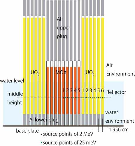
For the calculation, a three-dimensional model of the critical lattice of plutonium and uranium mixed oxide (MOX) and uranium dioxide (UO₂) fuel rods was prepared, as shown in Figure 2. This model is originally based on the mocked-up lattice in the TCA facility of the Japan Atomic Energy Research Institute [27]. The ²³⁵U enrichment of the UO₂ fuel is 2.6 wt%, and the Pu content in the MOX fuel is 3.0 wt%. The MOX is a semi-sintered fuel with a density of 6.06 g/cm³. Diameters of the MOX and UO₂ rods are 1.223 and 1.417 cm, respectively. In this model, the fuel rods are loaded vertically in a square-shaped lattice of pitch 1.956 cm. The central 9 × 9 part houses the MOX fuel, and 21 × 21 UO₂ rods surround them. The criticality is attained by feeding light water from the bottom of the tank to the appropriate level. In the condition, the lower part of the fuel is immersed in water, and the upper part of the fuel rods is in dry air.

Figure 2. Schematic view of MOX-UO₂ fuel assembly used for verification.

Parameter k_p was calculated for several water levels by solving

(34) $\mathcal{L}{\phi }_p=\frac{1}{k_p}{\mathcal{F}}_p{\phi }_p$(34)

by the k-power iteration with the MCNP-5 code, assuming no delayed neutron emission. For the calculation, 500,000 neutrons were employed per cycle, and the k_p was averaged over 800 cycles of calculations after skipping 200 cycles. The error was less than 5 pcm. The water level that gives k_p = 1 was interpolated as 51.057 cm.

I_α and I_FP,p were calculated for source points: 1) 2 MeV isotropic source at the center of fuel pins and at the middle height of the water level, 11 points; 2) 25 meV isotropic source in the water gap between the fuel rods, 11points. The positions are drawn in Figure 2. The adjoint flux I_α and I_FP,p (also I and I_FP in section 3.2) depend on direction Ω, but in this manuscript, the integrated quantities over all solid angle were calculated.

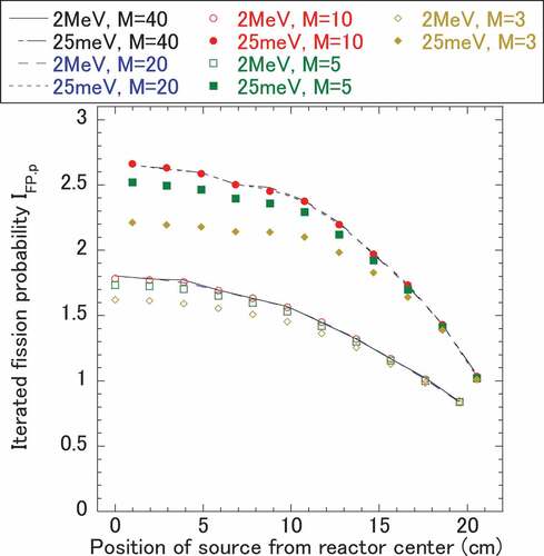
I_FP,p was calculated by the k-power iteration (kcode mode in MCNP-5), starting from each source without delayed neutron emission. Nominally, 1,000,000 neutrons were employed per cycle. k_p is estimated as e_p,m by neutron transport in every cycle m. The product of e_p,m up to cycle M was used as I_FP,p.

(35) $I_{FP,p}=\prod _{m=1}^M{e}_{p,m}$(35)

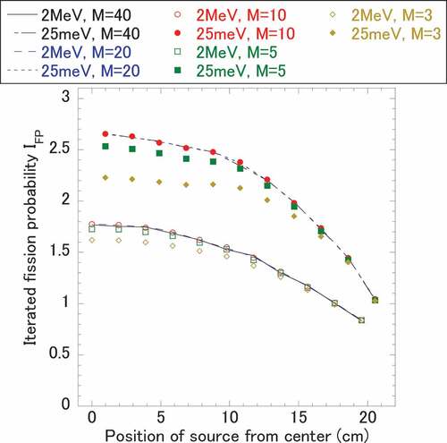
In Figure 3, the convergence of I_FP,p in relation to M is shown. The spatial distribution of I_FP,p is converged for M larger than 10. For M less than 10, the distribution differs from the converged one. Then, I_FP,p for M = 10 was used as the reference for I_a.

Figure 3. Convergence of iterated fission probability for prompt critical case.

For each source, a fixed source calculation without delayed neutron emission was performed to obtain I_α. For each source point, 1,000,000 neutrons were employed. The neutron transport was calculated until 1 ms after the source was placed. Since the generation time Λ of the core for the delayed critical condition was calculated to be 39 μs [11], 1 ms corresponds to 25 cycles, nominally. By this time limit, the total number of the descendant neutrons for a source was kept within 70. If the number were to increase, the calculation might fail owing to the exhaustion of the computation memory. In order to estimate I_α, the neutron flux integrated over all fuel pellets was taken for a certain time period after the sources were placed. Here it should be noted that distribution of I_α can be quantified with a local flux if the fluctuation of it is small and the neutron flux is dominated by the fundamental mode. To take the integration of the flux is just a way to reduce the fluctuation.

The spatial distribution of I_α evaluated from the integrated neutron flux within the time ranges of 100–150 μs, 200–300 μs, and 450–750 μs was normalized for all source points and compared with that of I_FP,p in Figure 4. In the time range of 100–150 μs, a slight difference is found. However, in the time region after 200 μs, very good agreement is found between the distributions of I_α and I_FP,p.

Figure 4. Comparison of I_α and I_FP,p for prompt critical case.

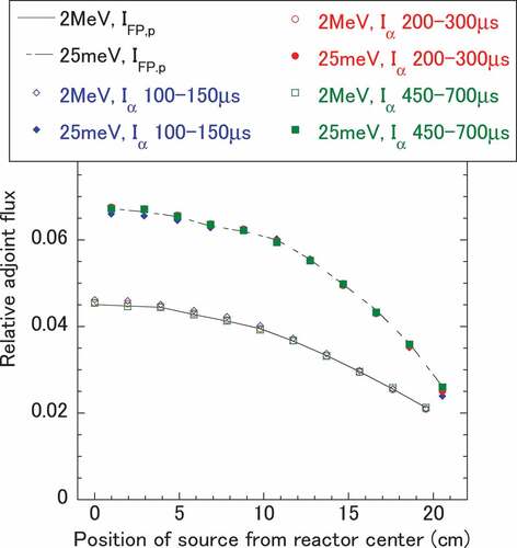
The results show that the distribution of φ_α^† can be estimated by the time-dependent neutron transport calculation without delayed neutron emission.

These calculations were performed with the published MCNP-5 without any modification.

3.2. Verification for delayed critical case

In this section, a comparison of the distribution of φ_ω^† to that of φ_k^† in the delayed critical case was performed by calculating I and I_FP for the sources. The water level in the MOX-UO₂ core in Figure 2 corresponding to the delayed critical state was surveyed to be 48.628 cm by the conventional k-power iteration calculation with delayed neutron emission.

For each source point mentioned in Section 3.1, I_FP was calculated with the kcode mode of MCNP-5, in which the delayed neutron source was radiated simultaneously with the prompt neutrons. Nominally, 1,000,000 neutrons were employed per cycle. As in the case of I_FP,p, convergence of the distribution of I_FP is found in cycle 10, as shown in Figure 5. The distribution and convergence of I_FP are very similar to those of I_FP,p. That is reasonable because the delayed neutron fraction is less than 1% of the fission source emission.

Figure 5. Convergence of iterated fission probability for delayed critical case.

In order to calculate I(r, E, Ω) by the time-dependent neutron transport calculation, the delayed neutron emission must be considered. Particularly to meet the requirement of Equation (25)(25) $exp\left(-\left(\omega +{\lambda }_j\right)t\right)\to 0$(25) , the time range of the calculation should be extended to hundreds of seconds, as the half-lives of the precursors are as high as 55 s [25]. Different from the case to calculate I_α in Section 3.1, continuing the transport calculation up to the time range by the fixed source calculation is very difficult, because over tens of thousands of cycles for the fission reaction chain are required for a source [20]. In MCNP-5, the neutron emission data are stored in a bank on computer memory. For the long family line of the fission chain, the memory is exhausted.

Nauchi developed TDPI [20]. TDPI is essentially the k-power iteration calculation of neutron transport from a point source, although the neutron flight time over cycles is summed up from the time an initial source is placed. The decay time of the precursors is stochastically sampled and added to the summation of the neutron flight time. In a conventional k-power iteration, k_eff is estimated as e_m by neutron transport calculation in cycle m − 1. In the iteration, the number of neutron emissions per fission in cycle m to make source in cycle m + 1 is normalized by e_m to control the population of the source [5]. Accordingly, the neutron flux tally in the time range t₁ to t₂ in cycle M, tally_M(t₁~ t₂), is evaluated for the normalized source size. Then, the time-dependent neutron flux can be estimated as

(36) $\psi \left(t_1\sim t_2\right)=\sum _{M=1}^{\mathrm{\infty }}tall{y}_M\left(t_1\sim t_2\right)\prod _{m=1}^{M-1}{e}_m$(36)

To obtain Ψ(t₁~ t₂), tally_M(t₁~ t₂) is output at each cycle as well as e_m. In the power iteration with MCNP-5, the fission source information is dumped onto a file at each cycle. Then, a restart calculation with the source is performed. By dividing the long family line into short segments, the neutron transport can be calculated up to some number of cycles without the issues of computation memory and the limitation of neutron sources (2³¹ for MCNP-5).

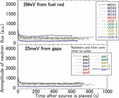
For each source point mentioned in Section 3.1, the TDPI calculation was performed with the enhanced MCNP-5 to obtain the time-dependent neutron flux Ψ integrated over all fuel pellets in the core. For the calculation for each source point, 2,000,000 neutrons were nominally employed per cycle, and 500 cycles of calculations were performed for a single run, followed by the creation of the source file. Starting from the source, the next run of 500 cycles was performed. This process was repeated 40 times for each source. By cycle 40 × 500 = 20,000, all source neutrons had been radiated more than 510 s after the initial source was placed. In other words, time-dependent neutron flux Ψ was estimated up to 510 s. For the 40 runs, the used CPU time was typically 102 days. To perform this computation, parallel calculations with the message passing interface were employed on the HPE SGI 8600, which is equipped in CRIEPI.

The time-dependent change in the amplitudes of neutron flux Ψ for each source is shown in Figure 6. In general, Ψ decreases rapidly within 40 s and becomes almost stable with time in the delayed critical state, although statistical fluctuation is found for some sources. For some sources, the time-dependent amplitude of the neutron flux is estimated up to 860 s; however, the shortest one is completed in 510 s. This time is when the earliest neutron among the 2,000,000 is emitted. The difference in the times is due to the stochastic nature of delayed neutron sampling in a family line of the fission reaction chain.

Figure 6. Time dependent variation of total neutron flux calculated for 22 source points shown in Figure 2.

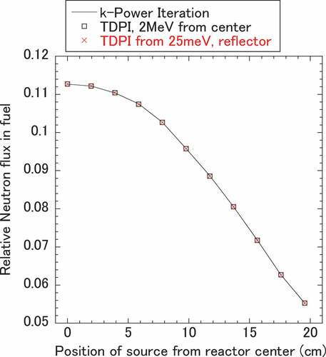
Subsequently, the convergence of the spatial neutron flux to the fundamental mode was checked. During the TDPI calculation, the time-dependent neutron flux Ψ in MOX and UO₂ fuels pins in the time region of 200–400 s was evaluated for two source points: 2 MeV source at the center of the core and 25 meV source in the reflector in Figure 2. The distributions of the flux are compared with those of the neutron flux φ_k by the conventional k-power iteration in Figure 7. The distributions of both Ψ and φ_k agree well with each other. As φ_k and φ_ω are similar in the delayed critical case, the time-dependent neutron flux Ψ originating in the two sources were considered to have converged to that of the fundamental mode of the natural mode equation, φ_ω. That means that Equation (6)(6) $\psi \to {\phi }_{\omega }{P}_{\omega }\left(t\right)={\phi }_{\omega }{P}_{\omega ,0}{e}^{\omega t}$(6) is satisfied.

Figure 7. Comparison of spatial distribution of flux: φ_k by k-power iteration and φ_ω by TDPI.

The tallied neutron flux for all fuel pins corresponds to I. The relative distribution of I for all source points is compared with that of I_FP in Figure 8. To obtain I, eight independent calculations were performed, changing the initial seed of the random number sequence for each source point. The average and standard deviation of the time-dependent amplitude of the neutron flux over the different random number sequences were taken.

Figure 8. Comparison of I by TDPI calculation to iterated fission probability I_FP.

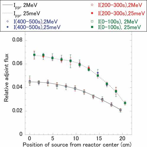
The calculated distribution of I agrees well with that of I_FP within the range of the error of I. Although the time change rate of the amplitude of the neutron flux does not stabilize within 50 s after the source is placed, the distribution of I in the time region from 0 to 100 s converges well. From the results, an insufficient length of time for Equations (6)(6) $\psi \to {\phi }_{\omega }{P}_{\omega }\left(t\right)={\phi }_{\omega }{P}_{\omega ,0}{e}^{\omega t}$(6) and (25(25) $exp\left(-\left(\omega +{\lambda }_j\right)t\right)\to 0$(25) ) seems to be insignificant for this problem. The error bars increase with time, perhaps because of the pile up effect of errors in the neutron multiplication discussed in a previous study [20].

Theoretically, the adjoint flux φ_ω^† satisfying Equation (9)(9) $\frac{\omega }{V}{{\phi }_{\omega }}^{†}=-{\mathcal{L}}^{†}{{\phi }_{\omega }}^{†}+{{\mathcal{F}}_p}^{†}{{\phi }_{\omega }}^{†}+{\sum }_j\frac{{\lambda }_j}{\omega +{\lambda }_j}{{\mathcal{F}}_{d,j}}^{†}{{\phi }_{\omega }}^{†}$(9) is similar to φ_k^† satisfying Equation (31)(31) ${\mathcal{L}}^{†}{{\phi }_k}^{†}=\frac{1}{k_{eff}}{\mathcal{F}}^{†}{{\phi }_k}^{†}$(31) in the delayed critical state. The proportional relation of I_FP to φ_k^† has already been proven theoretically and confirmed numerically [9–11]. From the excellent agreement of the distributions of I and I_FP, shown in Figure 8, the theory of the proportional relation of I to φ_ω^† and the calculation method of I to estimate φ_ω^† were verified.

4. Conclusion

The reciprocal of the reactor period, ω, is known to be the dominant eigenvalue of the natural mode equation. Recently, the relation of a perturbation introduced to a core to ω has been the focus to validate the reactor analysis methods and used cross sections because ω is directly measurable in any neutron multiplication state. The flux and adjoint flux of the natural mode equation relate such a perturbation to ω. Thus, calculation techniques of the adjoint flux have been studied recently.

Under these circumstances, the implication of the adjoint flux was clarified theoretically as the quantity proportional to the amplitude of the neutron flux after a sufficiently long time t after a source is placed at a phase space position where the adjoint flux is desired. In this time, the neutron flux distribution should converge to that of the fundamental mode of the natural mode equation, and exp(-(ω + λ)t) → 0, where λ is the decay constant of the precursor. This theoretical derivation extends the Bell and Glasstone study by considering the time delay of the delayed neutron emission. In addition, analogous and different points of the adjoint flux to that of the k-eigenvalue equation were well clarified.

Based on the theory, the amplitude of the neutron flux proportional to the adjoint flux can be estimated by continuous energy Monte Carlo time-dependent neutron transport calculations. For a three-dimensional model of prompt and delayed critical lattice that consists of MOX and UO₂ fuel rods moderated and reflected by light water, the amplitude of the neutron flux was calculated, employing the recently developed TDPI technique. The distributions of the calculated amplitudes agree well with those of the iterated fission probability for the prompt and delayed critical states. As the adjoint flux of the natural mode and k-eigenvalue equations are similar in the delayed critical state, the estimation method of the adjoint flux of the natural mode equation by way of TDPI calculation was verified.

Verification of TDPI calculations of ω and φ_ω^† for the non-critical states is now under study [24] by comparison of the present method to the G-IFP method by Jinaphnah and Zoia [24]. Very good agreements between the two methods in a multi-energy group have already been presented [19]. After the verification studies, verification studies would be extended to problems where the forward and adjoint flux take quite different shapes of distribution. Also, a validation study of the calculation techniques against the actual experimental data will be launched.

Disclosure Statement

No potential conflict of interest was reported by the author.

Notes

1. It is also called the ω-mode or α-mode equations.

2. For simplicity, the perturbation of λ is neglected here.

References

- Keepin GR. Physics of nuclear kinetics. U.S.: Addison Wesley Publishing Company, Inc; 1965.
- Stacey WM. Space-time nuclear reactor kinetics. New York (NY): Academic Press; 1969.
- Endo T, Yamamoto A. Sensitivity analysis of prompt neutron decay constant using perturbation theory. J Nucl Sci Technol. 2018;55(11):1245–1254.
- Jinaphanh A, Zoia A. Perturbation and sensitivity calculations for time eigenvalues using the generalized iterated fission probability. Ann Nucl Energy. 2019;133:678–687.
- X-5 Monte Carlo team. MCNP–a general Monte Carlo n-particle transport code version 5. Los Alamos (NM): Los Alamos national laboratory; 2003. (LA-UR-03-1987).
- Nauchi Y, Kameyama T. Calculation of iterated fission probability proportional to adjoint flux by continuous energy Monte Carlo method (1) Algorithm to calculate IFP. Proceedings of 2009 spring meeting of Atomic Energy Society of Japan; Mar 23–25; Tokyo, Japan: Tokyo Institute of technology. p. K40.
- Nauchi Y, Kameyama T. Calculation of iterated fission probability proportional to adjoint flux by continuous energy Monte Carlo method (2) Calculations of kinetic parameters weighted by IFP. Proceedings of 2009 spring meeting of Atomic Energy Society of Japan; Mar 23–25; Tokyo, Japan: Tokyo Institute of technology. p. K41.
- Kiedrowski BC, Brown FB. Adjoint-weighted kinetics parameters with continuous-energy Monte Carlo. Trans Am Nucl Soc. 2009;100:297–299.
- Ussachoff LN. Equation for the importance of neutrons, reactor kinetics and the theory of perturbations. Proceedings of Int. Conf. on the Peaceful Uses of Atomic Energy. Vol. 5; 1956 Aug 8–21; Geneva, Switzerland. p. 503–510.
- Hurwitz H. Naval reactor physics handbook. U.S.: U.S.Atomic Energy Commission; 1964.
- Nauchi Y, Kameyama T. Development of calculation technique for iterated fission probability and reactor kinetics parameters using continuous energy Monte Carlo method. J Nucl Sci Technol. 2010;47(11):977–990.
- Kiedrowski BC, Brown FB, Wilson PPH. Adjoint-weighted tallies for k-eigenvalue calculations with continuous-energy Monte Carlo. Nucl Sci Technol. 2011;168(3):226–241.
- Shim H, Kim C. Adjoint sensitivity and uncertainty analyses in Monte Carlo forward calculations. J Nucl Sci Technol. 2011;48(12):146–1453.
- Raskach KF, Blyskavka AA An experience of applying iterated fission probability method to calculation of effective kinetics parameters and keff sensitivities with Monte Carlo. proceedings of PHYSO2010; May 9–14; Pittsburgh, Pennsylvania.
- Truchet G, Leconte P, Peneliau Y et al.. Continuous-energy adjoint flux and perturbation calculation using the iterated fission probability method in Monte Carlo code TRIPOLI-4® and underlying applications. Proceedings of SNA + MC 2013; Oct27–31; Paris, France.
- Terranova N, Zoia A. Generalized iterated fission probability for Monte Carlo eigenvalue calculations. Ann Nucl Energy. 2017;108:57–66.
- Bell GI, Glasstone S. Nuclear reactor theory. Malabar (FL): Krieger Publishing co., Inc; 1970.
- Nauchi Y. Adjoint function satisfying alpha eigenvalue equation and iterated fission probability. Proceedings of 2018 autumn meeting of Atomic Energy Society of Japan; Sep 5–7; Okayama, Okayama, Japan. p.2M17.
- Nauchi Y, Jinaphanh A, Zoia A. Verification of adjoint functions of natural mode equation by generalized iterated fission probability method and by analog Monte Carlo. Proceedings of M&C 2019; Aug 25–29; Portland, (OR).
- Nauchi Y. Estimation of time-dependent neutron transport from point source based on Monte Carlo power iteration. J Nucl Sci Technol. 2019;56(11):996–1005.
- Nauchi Y. Attempt to estimate reactor period by natural mode eigenvalue calculation. Proceedings of SNA + MC 2013; Oct 27–31; Paris, France.
- Josey CJ, Brown FB. A new Monte Carlo alpha-eigenvalue estimator with delayed neutrons. Transactions of the American Nuclear Society. Vol. 118; 2018; Philadelphia, PA. p. 903–906.
- Zoia A, Brun E, Damian F, et al. Monte Carlo methods for reactor period calculations. Ann Nucl Energy. 2015;75:627–634.
- Nauchi Y, Jinaphanh A, Zoia A. Analysis of time-eigenvalue and eigenfunctions in the CROCUS benchmark. Proceedings of PHYSOR2020; Mar 29–Apr 2; Cambridge, UK.
- Hagura H, Okumura K, Iwamoto Y, et al. Development of neutron, photon and electron transport libraries. Proceedings of 2012 autumn meeting of Atomic Energy Society of Japan; Sep 19–21; Saijo, Hiroshima, Japan. p. I28.
- Shibata K, Iwamoto O, Nakagawa T, et al. JENDL-4.0: a new library for nuclear science and engineering. J Nucl Sci Technol. 2011;48(1):1–30.
- Tsuruta H, Kobayashi I, Suzaki T, et al. Critical sizes of light water moderated UO2 and PuO2-UO2 lattices. Tokai, Ibaraki, Japan: Japan Atomic Energy Research Institute; 1978. (JAERI 1254).