Development of local-scale high-resolution atmospheric dispersion model using large-eddy simulation part 6: introduction of detailed dose calculation method

ABSTRACT

We developed a LOcal-scale High-resolution atmospheric DIspersion Model using Large-Eddy Simulation (LOHDIM-LES) for the safety assessment of nuclear facilities and emergency responses to accidental or deliberate releases of radioactive materials. In parts 1–5 of this series, the basic performance was examined by comparing with wind tunnel or field experimental results on plume dispersion over various complex surface geometries under ideal and realistic atmospheric conditions. In this study, we introduced a dose calculation method that can simulate air dose rate distributions by considering shielding effects and inhomogeneous distribution of radioactive materials in the air and on the ground and building surfaces. First, we conducted LESs of radioactive plume dispersion and dry deposition in building array and investigated the basic performance of the dose calculation method by comparison with that of Monte-Carlo based three-dimensional radiation transport simulations by Particle and Heavy-Ion Transport code System (PHITS). Then, we compared the LOHDIM-LES results with actual air dose rate obtained from the monitoring posts in a nuclear facility. The observed data were reasonably simulated. Thus, we completed LOHDIM-LES, which can simulate plume dispersion, dry deposition, and air dose rates from complex distributions of radionuclides considering the influence of individual buildings under realistic meteorological conditions.

KEYWORDS:

• LOHDIM-LES
• PHITS
• SIBYL
• nuclear emergency response system
• large-eddy simulation
• plume dispersion
• gamma-ray dose
• dose-response matrix
• dose-attenuation matrix
• building shielding effects

1. Introduction

In local-scale atmospheric dispersion problems, an important issue is the accurate analysis of airborne radioactive materials released from nuclear facilities for safety and consequence assessment. At distances of up to several kilometers from the emission source, inhomogeneous distributions of air concentration and surface deposition around the evaluation point should be investigated considering the turbulent effects induced by individual buildings and local terrain variability. Another issue is the potential problem of hazardous materials being intentionally released in populated urban areas. Actual urban surface geometries are complex because grounds are highly inhomogeneous and covered with low- and high-rise buildings with various heights. In such a situation, the possible spatial distributions of contaminant plumes should be predicted considering the arrangements and sizes of individual buildings and obstacles in urban areas.

Computational simulation is an effective tool for estimating plume dispersion in the atmosphere. Japan Atomic Energy Agency (JAEA) has developed the System for Prediction of Environmental Emergency Dose Information (SPEEDI) for emergency response to domestic nuclear accidents [1]. A worldwide version of SPEEDI (WSPEEDI) has been constructed to expand the function of SPEEDI [2]. These systems consist of a mesoscale meteorological (MM) model and a Lagrangian particle dispersion model, which can provide near-real-time predictions of mean air concentrations, surface depositions of radionuclides, and radiological doses in a regional scale of approximately 100 km × 100 km with a grid resolution of several hundred meters. Although the accuracy of MM models for meteorological phenomena is continuously improving, they cannot reproduce small-scale turbulent flows due to the effects of buildings and structures, which are not explicitly resolved in MM models.

With the rapid development of computational technology, computational fluid dynamics (CFD) models have also been recognized as a helpful tool and been evolving as an alternative to wind tunnel experiments. In principle, there are two approaches to simulate turbulent flows: Reynolds-Averaged Navier-Stokes (RANS) and Large-Eddy Simulation (LES) models. RANS-based CFD models calculate a mean wind flow to deliver an ensemble- or time-averaged solution, and all turbulent motions are modeled using turbulence parameterization. The main advantage of the RANS model is its efficiency in simulating a mean flow field at a relatively low computational cost. Sada et al. [3] designed a RANS-based CFD model for simulating the plume dispersion of radioactive materials around nuclear facilities and showed the basic performance in comparison with wind tunnel experiments. Recently, LES-based CFD models have also become useful tools. The basic idea of LES models resolves large-scale turbulent motions and parameterizes only small-scale motions. The advantage is that they can capture the unsteady characteristics of turbulent flows and the dispersion process over complex surface geometries. Therefore, we developed the LES-based CFD model called local-scale high-resolution atmospheric dispersion model using LES (LOHDIM-LES).

In our previous studies, the performance of LOHDIM-LES was evaluated by conducting detailed simulations of turbulent flows and plume dispersion over a flat terrain and a two-dimensional hill, around an isolated building, within building arrays with different obstacle densities, and within a central district of an actual urban area [4–8]. We showed that the model’s basic performance was comparable to wind tunnel experiments, and completed the basic version of LOHDIM-LES [9]. Ono et al. [10] also conducted LESs of plume dispersion over a hilly terrain considering the effects of plume rise, surrounding buildings, and geophysical features, and showed the high applicability of the LES model to the environmental impact assessment of geothermal power plants as an alternative to wind tunnel experiments. However, these conventional LES models are applicable only to ideal meteorological conditions, in which mean wind velocities and directions are constant (similar to those in wind tunnel experiments). Real atmospheric flows are composed of not only turbulence but also meteorological disturbances that have various types of atmospheric motions with different time and spatial scales. Therefore, we developed an approach that can be coupled with an MM model to represent both small-scale turbulent winds and meteorological disturbances [11] and evaluated this new calculation method using the field experimental data of Joint Urban 2003, which was conducted in the central district of Oklahoma City. Our findings showed that LOHDIM-LES coupled with an MM model reasonably simulates the mean and fluctuating concentrations of plumes in complex surface geometries under real meteorological conditions [12]. Thus, LOHDIM-LES had a broad range of purposes; it can be used not only for the safety assessment of nuclear facilities as an alternative to wind tunnel experiments but also for analyses of plume dispersion in urban areas under realistic meteorological conditions.

In this study, which is the last step of the model development, we incorporated a dose calculation method into LOHDIM-LES. Three-dimensional radiation transport should be simulated considering shielding effects in estimating air dose rates from the inhomogeneous distribution of radioactive materials induced by individual buildings and structures. These processes are not sufficiently considered in the operational models of JAEA (SPEEDI and WSPEEDI). In WSPEEDI, air dose rates are estimated by multiplying the air concentration and surface deposition of radionuclides at the estimation point by conversion factors. This treatment is applicable to the calculation grid of WSPEEDI (larger than 1 km) and to estimation points located farther than several kilometers from the release point. In SPEEDI, the distribution of a radioactive plume is simulated by a large number of marker particles that contain the radioactivity of the released radionuclides, and air dose rates are estimated by summing up the dose contributions of all the particles. A lookup table of dose-response matrices, which are functions of the distance between a particle and an evaluation point, the altitude of a particle above a ground surface, kinds of radionuclides, and a target age, is used to quickly calculate the air dose rate contribution of each particle. For air dose rates produced by surface deposition, the treatment is the same as that for WSPEEDI. However, the shielding effects of individual buildings are not considered in SPEEDI or WSPEEDI.

Detailed dose calculation considering shielding effects can be achieved only by a sophisticated simulation code, such as Particle and Heavy-Ion Transport code System (PHITS) [13]. Recently, Satoh et al. [14,15] developed a calculation method that can quickly and accurately estimate air dose rates from inhomogeneous distributions of radioactive materials in the environment by using a dataset of dose-response matrices based on prior PHITS simulations. The calculation code with this new method, called SImulation code powered BY Lattice dose-response functions (SIBYL), performed well in estimating air dose rate distributions using outputs of LOHDIM-LES simulations; its results were comparable with PHITS results [15]. Thus, we incorporated SIBYL as the dose calculation module into LOHDIM-LES.

To evaluate the performance of LOHDIM-LES integrated with a detailed dose calculation method that considers shielding effects, we conducted LESs of plume dispersion and estimated the air dose rates produced by a radioactive plume of actual radionuclides released from a nuclear facility. Our objective was to validate the model’s basic performance in estimating air dose rates from inhomogeneously distributed radionuclides in plumes under the influence of buildings and structures in comparison with environmental monitoring post (MP) data from the vicinity of the nuclear facility.

2. Model description

The LOHDIM-LES code was designed based on the LES model to perform detailed simulations of the unsteady behaviors of complex turbulent flows and plume dispersion considering local terrain variability and individual buildings, which are explicitly resolved at a fine grid resolution. The dose calculation module SIBYL was incorporated into LOHDIM-LES. In this chapter, we briefly outline the LES dispersion model, the SIBYL module, and the calculation flow of the coupling system. Details about the dose calculation method are given elsewhere [15].

2.1. Outline of LOHDIM-LES

The governing equations of LOHDIM-LES are the filtered continuity, Navier-Stokes under Boussinesq approximation, and transport equations of temperature and concentration. The coupling algorithm of the velocity and pressure fields is based on the marker-and-cell method [16] with the second-order Adams-Bashforth scheme for time integration. The Poisson equation is solved by the successive over-relaxation method. These equations are solved based on a Cartesian grid system consisting of horizontally uniform and vertically stretched grid spacings of an order of 1 m. The subgrid-scale (SGS) turbulent effect is represented by the standard Smagorinsky model [17]. SGS scalar fluxes are also parameterized by an eddy viscosity model. The turbulent effects of buildings and local terrain are represented by the immersed boundary method [18]. The forest canopy effect is represented by a drag force term. The dry deposition is calculated from the deposition velocity and air concentration on ground and building surfaces. Details about the governing equations are described in Appendix A.

A crucial issue in appropriately driving the LES model to simulate plume dispersion in the atmosphere is how to generate turbulent boundary layer (TBL) flows with small-scale turbulent fluctuations, since the model calculates instantaneous values. LOHDIM-LES can reproduce two typical atmospheric conditions: idealized atmospheric conditions (such as wind tunnel flows) and realistic meteorological conditions. For the idealized atmospheric condition, a representative mean wind velocity profile is given to the inflow boundary, and TBL flows with small-scale turbulent fluctuations are reproduced by means of the turbulent inflow technique and/or roughness obstacles placed upstream in the development section in the computational domain. This approach is designed based on wind tunnel experiments for the construction of nuclear facilities in Japan [19]. For the real meteorological condition, coupling with an MM model and observations (OBS) is effective. The meteorological data are used to supply the initial and boundary conditions, and realistic atmospheric turbulence is generated by the turbulent inflow technique. This coupling approach can be used to better understand the atmospheric dispersion process of a tracer gas under varying atmospheric conditions in post analysis of accidental or deliberate releases of radioactive materials. Details about the coupling with OBS are described in Appendix B.

By resolving complex heterogeneous surface geometries at a fine grid resolution and using different approaches in accordance with target atmospheric conditions, LOHDIM-LES can simulate the unsteady behaviors of plume dispersion and capture peak concentrations in homogeneous turbulent flow fields induced by individual buildings under ideal and realistic meteorological conditions.

2.2. Dose calculation method

To quickly and accurately estimate dose distributions considering the shielding effects of buildings, we employed a calculation method that uses dose-response matrices [14]. The dose rate calculation code SIBYL [15] was developed to estimate the dose rate distributions at the study site from the air concentration and surface deposition of a specific nuclide, which were provided by LOHDIM-LES. The dose-response matrices represent the pre-evaluated conversion factors of the ambient dose equivalent rate and the air kerma free-in-air rate produced by radioactivity concentration of the nuclide per unit volume of air and per unit area of the ground at a height of 1 m above the ground. These matrices are evaluated by photon transport simulations with PHITS [13] to include three-dimensional particle transport phenomena, such as skyshine and groundshine.

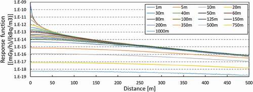
A dataset of dose-response matrices was generated for various radionuclides to apply the dose calculation method SIBYL to the LOHDIM–LES calculations. Each dose-response matrix was composed of a two-dimensional array of the dose contribution at a grid point in a horizontal square area around the center grid of each radiation source with a unit radioactivity of specific radionuclides. The domain size of the pre-evaluated dose-response matrices was 1001 m × 1001 m. This area was segmented into sections with a grid spacing of 1 m × 1 m in the horizontal direction and at several heights in the vertical direction. As an example, the dose-response functions of ⁸⁵Kr per unit volume of air at several heights are shown in Figure 1. The area is large enough to consider the dose contributions from distant radionuclides because the length from a radiation source corresponds to approximately 5 times of the mean-free-path of ¹³⁷Cs [14]. These functions were prepared for the radiation sources of ¹³⁴Cs, ¹³⁶Cs, ¹³⁷Cs, ¹³¹I, ¹³²I, ¹³³I, ¹³²Te, ⁸⁵Kr, and ¹³³Xe per unit volume of air at the altitudes of 1, 5, 10, 20, 30, 40, 50, 60, 80, 100, 125, 150, 200, 350, 500, 750, and 1000 m based on prior PHITS simulations; functions were also prepared for the same altitudes for these sources except ⁸⁵Kr and ¹³³Xe per unit area of the ground. The ¹³⁷Cs data included contributions from metastable ^137mBa in radioactive equilibrium. The air dose rates were normalized to a unit hour and had units of $mSv/h$ and $mGy/h$ in the pre-evaluated functions.

Figure 1. Response function of ⁸⁵Kr from a source region to the surroundings based on prior PHITS simulations

The air dose rates are calculated using the dataset of dose-response functions as follows. First, the surface deposition density $C_{dep}$ for an integration time from the plume release start time $T_{st\mathrm{\_}plume}$ to the end time $T_{en}$ and the mean air concentration $C_{air}$ at a cell during a given time period of $\mathrm{\Delta }{T}_{calc}$ from $T_{st}$ to $T_{en}$ are calculated as follows:

(1) $\begin{array}{rl}& C_{dep}\left(x_i,y_j,z_{wall}\right)={\sum }_{t=T_{st\mathrm{\_}plume}}^{T_{en}}\hspace{0.17em}\\ & {\left(V_d{\bar{\mathrm{c}}}_{wall}\left(x_i,y_j,z_{wall}\right)\mathrm{\Delta }t\right)}_t\end{array}$(1)

(2) $C_{air}\left(x_i,y_j,z_k\right)=\sum _{t=T_{st}}^{T_{en}}{\left(\bar{\mathrm{c}}\left(x_i,y_j,z_k\right)\mathrm{\Delta }t\right)}_t/T_{calc}$(2)

where $\mathrm{\Delta }t$, $V_d$, and ${\bar{\mathrm{c}}}_{wall}$ are the calculation time step, dry deposition velocity, and concentration at the first grid point above the ground and building surfaces $\left(z_{wall}\right)$, respectively. Then, the air dose rates are calculated by the matrices of the dose-response and dose-attenuation by buildings from the values of the surface deposition density and mean air concentration as the following equations, respectively.

(3) $\begin{array}{rl}& D_{dep}\left(x_i,y_j\right)=\sum _{l=-L}^L\sum _{m=-M}^M{d}_{dep}\left(l,m,0\right)C_{dep}\\ & \left(x_i+l,y_j+m,z_{wall}\right)a_{dep}\left(x_i,y_j,l,m,0\right)\end{array}$(3)

(4) $\begin{array}{rl}& D_{air}\left(x_i,y_j\right)=\sum _{l=-L}^L\sum _{m=-M}^M\sum _{n=1}^N{d}_{air}\left(l,m,n\right)C_{air}\\ & \left(x_i+l,y_j+m,n\right)a_{air}\left(x_i,y_j,l,m,n\right)\end{array}$(4)

where ${\mathit{D}}_{\mathit{d}\mathit{e}\mathit{p}}\left(x_i,y_j\right)$ and ${\mathit{D}}_{\mathit{a}\mathit{i}\mathit{r}}\left(x_i,y_j\right)$ are the air dose rates at the position of $\left(x_i,y_j\right)$ for the ground and cloud sources, respectively. $d_{dep}$ and $d_{air}$, and $a_{dep}$ and $a_{air}$ are the pre-evaluated dose-response and dose-attenuation matrices resized to the model grid, respectively. In the dose-response and dose-attenuation matrices, $l,m,\mathrm{a}\mathrm{n}\mathrm{d}n\mathrm{a}\mathrm{r}\mathrm{e}$ coordinates, whereas $-L\mathrm{t}\mathrm{o}L,-M\mathrm{t}\mathrm{o}M,\mathrm{a}\mathrm{n}\mathrm{d}1\mathrm{t}\mathrm{o}N$ are mesh numbers. These matrices are designed to adapt the computational mesh of LOHDIM-LES by a linear interpolation in the horizontal direction and a logarithmic interpolation in the vertical direction from the original matrices under the assumption that gamma rays passing through the air layer are exponentially decreased. The horizontal mesh numbers ($L,M$) are changed depending on the horizontal computational grid resolution by keeping the 1001 m × 1001 m area of the original matrices. The vertical mesh number ($N$) is the same as the vertical computational mesh. For example, the number of resized cells in the $l$ direction is expressed by $L=500/\bar{\mathrm{\Delta }}$. Here, $\bar{\mathrm{\Delta }}$ is the grid spacing of the computational model.

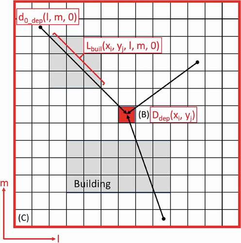
Figure 2 shows a schematic of the calculation of the air dose rate distributions produced by surface deposition as an example. $2L+1$ and $2M+1$ indicate the horizontal mesh size of the dose-response matrix resized to the model grid of LOHDIM-LES in the $l\mathrm{a}\mathrm{n}\mathrm{d}m$ directions, respectively. The dose rate distribution at the target area (A in Figure 2) is estimated using the dose-response matrix and the distribution map of deposited radioactivity. The dose rate at the target cell (B in Figure 2) is determined by summing up the dose contributions from the source cells in the dose-response function domain (C in Figure 2). The same operation is applied to the other sections of the mesh whose surface deposition is inside the LOHDIM-LES calculation area (D in Figure 2). Note that the entire target area is inside the calculation area (D in Figure 2).

Figure 2. Schematic of the calculation of the dose rate distributions: (a) target area for estimating dose rate distribution; (b) target cell established in area (A); (c) region considering the dose contribution to the target cell (B); (d) LOHDIM-LES calculation area [15]

Figure 3 shows a schematic of the calculation of the dose-attenuation by buildings in the matrix area (C in Figures 2 and 3) produced by the surface deposition as an example. The building shielding effects are represented by using the following attenuation matrices:

(5) $a_{dep}\left(x_i,y_j,l,m,0\right)=exp\left(-\mu L_{buil}\left(x_i,y_j,l,m,0\right)\right)$(5)

(6) $a_{air}\left(x_i,y_j,l,m,n\right)=exp\left(-\mu L_{buil}\left(x_i,y_j,l,m,n\right)\right)$(6)

Figure 3. Schematic of the calculation of the dose rate distributions considering building shielding effects. (b) and (c) are the same as those in Figure 2

where $L_{buil}\left(x_i,y_j,l,m,0\right)$ and $L_{buil}\left(x_i,y_j,l,m,n\right)$ are the transmission distance through buildings between the positions of $\left(x_i,y_j\right)$ and $\left(l,m,0\right)$ and between $\left(x_i,y_j\right)$ and $\left(l,m,n\right)$ for the ground and cloud sources, respectively. $\mu$ is the attenuation coefficient. The dose rate at the target cell under the building shielding effects is also determined by summing up the dose contributions considering the attenuation by buildings. The same procedure is repeated for the other cells inside the target domain. For calculating the dose rate distribution produced by a radioactive plume, the dose rate at the target cell is determined by summing them up for the horizontal and vertical directions. Note that the build-up of gamma rays by the buildings is not considered in the present algorithm.

The total external dose $D_{total}$ is estimated by the following equation:

(7) $D_{total}\left(x_i,y_j\right)=D_{air}\left(x_i,y_j\right)+D_{dep}\left(x_i,y_j\right)$(7)

The second term on the right-hand side is not considered for the noble gases.

2.3. Calculation flow

Figure 4 illustrates the calculation flow of LOHDIM-LES incorporated with the dose calculation module SIBYL. The model solves the governing equations and then provides computed data of wind velocity, temperature, air concentration, and dry deposition. In the dose simulations, the SIBYL module is executed in a given time interval, and the mean air concentrations and/or surface deposition obtained from LOHDIM-LES are provided to the dose calculation module.

Figure 4. Calculation flow of LOHDIM-LES integrated with the dose calculation module SIBYL, which can be run with a postprocessing option

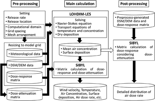
When executing LOHDIM-LES for radioactive plume dispersion, it is necessary to preprocess the meteorological data used for the model input, surface geometry data, dose-response matrix for specific radionuclides, and dose-attenuation matrix. Meteorological data are composed of MM model data or OBS data. Due to the coarse grid resolution on an order of km of MM models and limitations in the spatial resolution of OBS data, meteorological data are linearly interpolated and resized to the model grid based on the computational domain, grid spacing, and mesh arrangement. Surface geometry data are composed of digital elevation model (DEM) and/or digital surface model (DSM) data resolved by a high-resolution grid from the order of 1 m to 10 m and then resized to the model grid spacing. DEM and DSM are composed of the mesh data of the elevation and the ground surface height including the tops of roughness elements such as buildings, structures, and trees, respectively. The dose-response matrices are also resized as mentioned in the previous section. The dose-attenuation matrix is obtained based on the spatial distribution of building height data, which are estimated from the difference between the resized DSM and DEM data.

As seen in equations (5) and (6), the dose-attenuation matrix requires enormous computational data. In the sequential dose simulations by the SIBYL module from the LOHDIM-LES results of mean air concentrations and surface deposition, the air dose rates are obtained at several stationary points, such as monitoring posts, by preparing the dose-attenuation matrix for the corresponding measurement points. In the estimation of the spatial distributions of the air dose rates, the matrix calculation of the dose-response considering the dose-attenuation is executed by the SIBYL code as a postprocessor.

2.4. Verification of dose calculation method

The dose calculation method with building shielding effects was verified by comparing its results with those of Monte-Carlo based three-dimensional radiation transport simulations by PHITS. PHITS deals with the transport of nearly all particles, including neutrons, protons, heavy ions, photons, and electrons, over wide energy ranges using various nuclear reaction models and data libraries. It can provide the reference data used for verifying the SIBYL module. Since the details are already shown in Satoh et al. [15], the verification is only outlined here. We conducted LESs of radioactive plume dispersion and dry deposition in a regular array of cubic buildings in a fully-developed TBL flow. The air dose rates were estimated from the plume and surface deposition considering the shielding effects. The computational domain was 240 m × 240 m × 150 m in the streamwise, spanwise, and vertical directions, respectively. Each building had dimensions of 24 m × 24 m × 24 m. The cubic buildings were arranged in five rows and five columns over a flat terrain. Here, ¹³⁷Cs having a dry deposition characteristic was selected as a tracer gas to calculate air dose rates produced by the plume and surface deposition. The ground-level point source of ¹³⁷Cs was located at the center, behind the buildings in the second row. The total release amount of radioactivity was 347.25 Bq. According to the study of the sensitivity analysis by Pugh et al. [20], dry deposition velocities for building surfaces were determined in accordance with the particle size of airborne substances. Thus, the dry deposition velocities of fine particles are 0.05 cm/s for the concrete building surfaces, and those of coarse ones are 0.02 cm/s and 0.2 cm/s for the building walls and roof, respectively. Since ¹³⁷Cs can be classified into fine particles, the deposition velocity was set as 0.05 cm/s for the building surfaces, while that was set as 0.1 cm/s for the ground surfaces [2].

Figure 5 illustrates the spatial distributions of the air dose rates of ¹³⁷Cs at a height of 1 m, as obtained by PHITS and LOHDIM-LES with SIBYL from LES data of the time-averaged concentrations of the plume and surface depositions during the time period of 30-minute after the release. The differences of the air dose rates from the plume and the surface deposition calculated by LOHDIM-LES and PHITS lay in the range of 10% and 3%, respectively, for the high-dose downstream areas from the release point. On the other hand, there were comparatively larger differences between them for the low-dose areas behind the buildings upstream of the point source. Here, it is important to accurately estimate high-dose areas especially in the case of nuclear accidents. The accurate estimation for not only high-dose but low-dose areas is beyond the scope of the current study. For such a situation, Monte-Carlo based three-dimensional radiation transport simulations by PHITS should be utilized.

Figure 5. Spatial distributions of the air dose rates of ¹³⁷Cs produced by (a) the plume and (b) surface deposition at a height of 1 m. The circle indicates the point source location

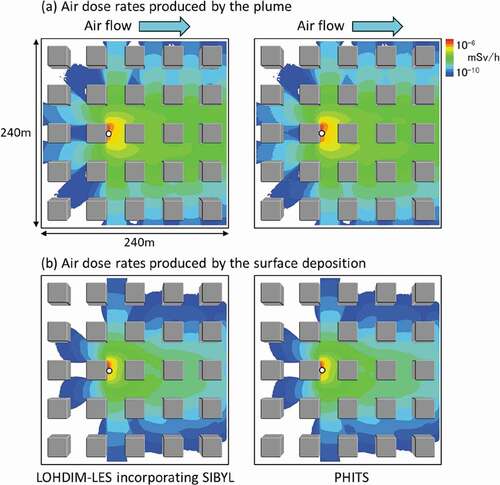
The computation time for estimating the air dose rates by the dose-response matrices was approximately 100 times faster than that of PHITS. These results show that the detailed dose calculation method considering building shielding effects can quickly and accurately estimate air dose rates at high-dose areas from inhomogeneous distributions of radioactive materials.

3. Validation using actual data obtained from nuclear facility

3.1. Study site and dataset of observations

To evaluate the dose calculation method using the dose-response matrices, we conducted LESs on the plume dispersion of radionuclides released from Rokkasho Reprocessing Plant (RRP), the nuclear fuel reprocessing plant in Rokkasho, Japan. The test operations of reprocessing were conducted using actual spent fuels at RRP from March 2006 to October 2008. When spent fuels are reprocessed, radionuclides, such as ⁸⁵Kr, ³H, ¹⁴C, and ¹²⁹I, are discharged into the atmosphere under release control. The air concentrations of these radionuclides and the air dose rates were also measured. These data were considered to be the only ones suitable for model validation.

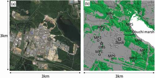
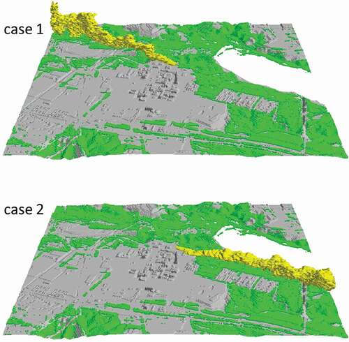
Figure 6 shows the study site in RRP. There are many buildings and structures within this site. Forest canopy surrounds the area, and Obuchi marsh is located at the east side. The ground cover is highly heterogeneous. The stack height is 150 m above ground level. The 10-minute averaged wind velocities were obtained at heights of 50 m, 75 m, 150 m, 250 m, and 300 m in the one-dimensional vertical direction with a 10-minute time interval by a Doppler sodar located about 700 m west of the plume stack. In order to estimate atmospheric stability, the wind velocities and solar radiation at 10 m above the ground-level, and the air temperature and net radiation at 2 m above the ground-level were obtained. Air concentrations and air absorbed dose rates were measured at the nine MPs at approximately 1 m height above the ground surface height including the tops of buildings and structures located around the plume stack. Increases in the air dose rate were mainly produced by ⁸⁵Kr. Since ⁸⁵Kr is non-reactive and non-depositing, the dry deposition scheme was not considered here, and the performance of the calculation method on the air dose rates from the plume in the atmosphere should be investigated.

Figure 6. Study site in the nuclear fuel reprocessing plant in Rokkasho. The photograph on the left is reproduced by Google Earth graphics. The figure on the right shows the computational area of the study site. The square, star, and circle depict the plume stack, meteorological observation station, and MPs, respectively

3.2. Simulation period

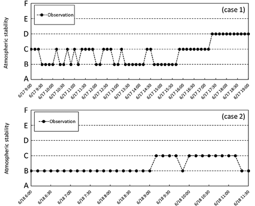
The target simulation periods were from 0900 JST to 1930 JST on 17 June 2008 and from 0600 JST to 1130 JST on 18 June 2008 for cases 1 and 2, respectively. These were periods wherein no precipitation and increase of ⁸⁵Kr air concentrations were detected at the MPs. The simulation results were compared with the OBS data of the meteorological observation, 10-minute mean ⁸⁵Kr air concentrations, and air dose rates provided by Japan Nuclear Fuel Limited (JNFL).

Figure 7 shows a time series of the atmospheric thermal stability during the two simulation periods. The atmospheric stability plays an important role in determining plume spreads emitted from the tall stack. The atmospheric stability was classified by Pasquill classes [19]. These classes are A (extremely unstable), B (moderately unstable), C (slightly unstable), D (neutral), E (slightly stable), and F (moderately stable). The atmospheric conditions frequently varied between B and C from 0900 JST to 1710 JST and became D from 1720 for case 1. By contrast, the atmospheric conditions for case 2 constantly showed B from 0600 JST to 0900 JST and almost showed C from 0900 JST. These may indicate that convective turbulent motions and/or local thermal plume were highly active early in the morning.

Figure 7. Time series of atmospheric stability during the two simulation periods (cases 1 and 2). The characters A-F indicate the atmospheric stability classes

3.3. Computational model

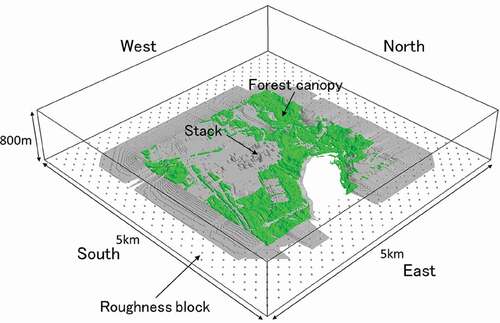
Figure 8 shows the computational model used to simulate the plume dispersion around RRP. The size of the computational domain was 5.0 km × 5.0 km in the horizontal direction at a depth of 800 m. The total mesh number was 1000 × 1000 × 105 nodes. The grid spacing was 5 m in the horizontal direction and 2.5–20 m stretched in the vertical direction. The surface geometries, buildings, and forest canopy were explicitly resolved using a DSM dataset (Kokusai Kogyo Co., Ltd.). The study site measured 3.0 km × 3.0 km in the horizontal direction, as shown in Figure 6 (b). Driver sections with a length of 1.0 km were set, and roughness blocks were placed to efficiently generate TBL flows as well as wind tunnel experiments. In order not to generate unrealistic separated turbulent flows, gentle-slopes were set toward each edge of the study site. Since a Cartesian grid system was adopted, the shape of individual buildings and structures was not strictly represented. However, it is clearly seen from Figure 6 (a) that the actual arrangements of the buildings, structures, and trees were represented well by a high-resolution grid using the DEM and DSM dataset. Therefore, this model setup was enough to simulate atmospheric turbulent flows in consideration of the actual surface geometry. The calculation time step was 0.05 s.

Figure 8. Computational model

3.4. Boundary conditions

The OBS 10-minute averaged wind velocities obtained at a stationary point were used to prescribe the inflow boundary conditions under the assumption of horizontal homogeneity. First, since the vertical resolution of the meteorological observations was limited, the OBS data were linearly interpolated on the vertical grids of the LES model and then imposed at the vertical planes of the inflow boundaries with a 1-minute time interval by interpolating them in the time direction. Then, the input data were modified under the assumption of a mean wind vertical profile with a power law exponent of 0.14 below a height of 50 m and above a height of 300 m. For fast turbulence development under realistic meteorological conditions, only the fluctuating components were extracted at a downstream station, and the fluctuations were added to the averaged winds prescribed at the inflow boundaries. Details about this turbulent inflow technique is described in Appendix B.

The atmospheric thermal stability was assumed to be neutral because the spatial resolution of the OBS data of the surface temperature was limited. However, the assumption of a neutral stability condition requires caution. For example, Moeng and Sullivan [21] conducted LESs of neutral and unstable TBL flows and investigated the difference between the turbulent structures. They reported that streaky structures are formed near the ground surface in cases of shear-dominated flows, and strong updrafts that are roughly comparable with the TBL scale are observed in cases of buoyancy-dominated flows. As seen from Figure 7, the atmospheric stability was unstable in most of the target simulation periods. The assumption of a neutral stability condition may induce calculation errors of plume spreads. Although turbulent structures under neutral and unstable conditions are essentially different, the time variation patterns of mean wind speeds and directions can be generally reproduced because OBS data are directly prescribed at the inflow boundaries under this calculation condition.

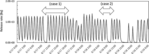
3.5. Plume release conditions

Figure 9 shows a time series of the release rates of ⁸⁵Kr during the two simulation periods. The rates varied approximately every hour except from 1000 JST to 1050 JST on June 17 and from 0910 JST to 1010 JST on June 18. The plume released from the stack rises due to the momentum and buoyancy of the stack gases. Many formulas have been proposed to predict the plume rise from a stack using meteorological information. According to a review paper on 26 plume rise formulations by Okamoto et al. [22], the optimized CONCAWE provides the best performance in comparison with actual plume rises by observations, although most of other formulations overestimate plume rise under low-wind-speed conditions [23]. The formulation is as follows:

(8) $\mathrm{\Delta }H=0.414{\left(1000Q_h\right)}^{0.444}/U_{stack}^{0.694}$(8)

(9) $Q_h=\frac{1}{4}\pi D^2{V}_s{\rho }_{gas}{C}_p{T}_{gas\mathrm{\_}air}$(9)

Figure 9. Time series of the ⁸⁵Kr release rate for the two simulation periods

where $\mathrm{\Delta }H$, $Q_h$, $U_{stack}$, $D$, $V_s$, ${\rho }_{gas}$, $C_p$, and $\mathrm{\Delta }{T}_{gas\mathrm{\_}air}$ are the plume rise above the stack, heat emission rate, wind speed at the stack height, stack inside diameter, stack velocity, effluent gas density, air specific heat capacity at constant pressure, and temperature difference between the effluent gas and ambient temperature, respectively. The $U_{stack}$ and the ambient temperature in $\mathrm{\Delta }{T}_{gas\mathrm{\_}air}$ were prescribed by the OBS values measured at the stack height A time series of the plume rise estimated by the optimized CONCAWE formulation is shown in Figure 10.

Figure 10. Time series of the plume rise estimated by the optimized CONCAWE formulation for the two simulation periods

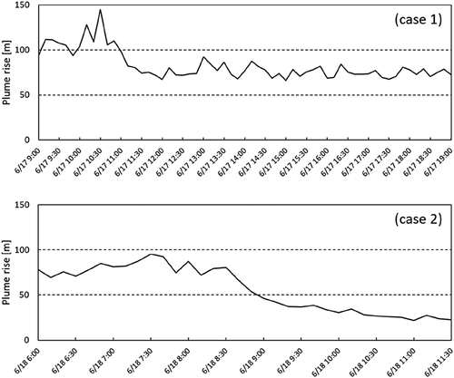
From 0900 JST to 1100 JST on June 17, the plume rise showed large values and indicated a particularly sharp peak at 1030 JST due to the weak wind conditions. From 0600 JST to 0850 JST on June 18, the plume rise ranged from 50 m to 100 m and then gradually decreased in the range of 25 m to 50 m due to the small difference in the temperature between the effluent gas and the ambient temperature (not shown here).

4. Results

4.1. Flow field

Figures 11 and 12 show time series of the wind speeds and directions at the stack height for the two simulation periods. For case 1, the OBS wind speeds increased with the development of the daytime convective boundary layer from 1030 JST and fluctuated by around 4 m/s with a time period of approximately 30 min to 1 h. The OBS wind directions also fluctuated by around 100 degrees. The mean wind flows from the east side were dominant. The fluctuation patterns of the LES wind speeds and directions were generally similar to those of the OBS data. For case 2, the OBS wind speeds also rapidly increased with the development of the daytime convective boundary layer from 0830 JST. The OBS wind direction was around 270 degrees from 0700 JST, which indicated that the mean wind flows from the west side were dominant. The LES overestimated the wind speeds, especially from 0800 JST to 0940 JST, while the LES wind direction data were similar to the OBS data. This was because the active convective turbulent motions were not represented well under the assumption of a neutral stability condition in this calculation. Except during this period, the LES data agreed well with the OBS data.

Figure 11. Time series of the wind speeds and directions at the stack height during the simulation period from 0900 JST to 1900 JST on 17 June 2008

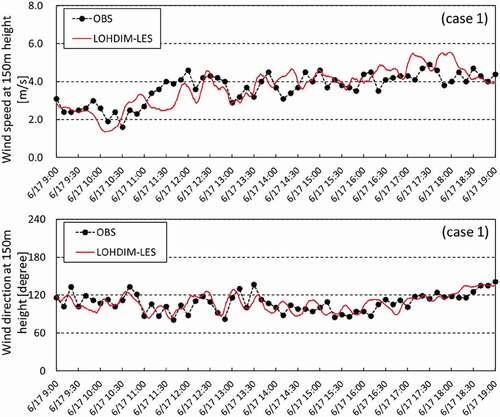
Figure 12. Time series of the wind speeds and directions at the stack height during the simulation period from 0600 JST to 1130 JST 18 June 2008

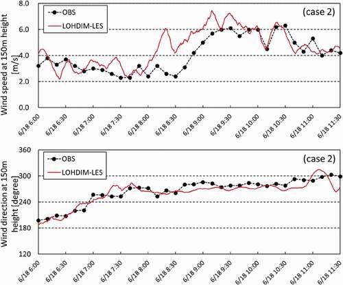
In particular, a large difference was observed in the wind speeds between the OBS and LES data for case 2 due to the assumption of a neutral stability condition. However, it is expected that the direction of plume transportation was accurately simulated, given that the general time variation patterns of the mean wind speeds and directions were reproduced well.

4.2. Air concentration field

Figure 13 shows instantaneous plume dispersion fields at 1730 JST on June 17 and 1040 JST on June 18 for the two cases. According to a schematic diagram of plume dispersion behaviors in the atmosphere by Davidson et al. [24], a plume is deflected by turbulent eddies larger than the scale of the plume close to the release point. Then, downstream from the release point, the plume gradually spreads, since its scale becomes comparatively larger than the scale of turbulent eddies. These main features of plume dispersion at downstream distances captured by LOHDIM-LES are similar to those illustrated by Davidson et al.

Figure 13. Instantaneous plume dispersion fields at 730 JST on 17 June 2008 (case 1) and 1040 JST on 18 June 2008 (case 2)

Figures 14 and 15 show time series of the 10-minute mean air concentrations of ⁸⁵Kr for the two cases. For case 1, the MP data of the mean concentrations were intermittently detected mainly at MP2 and MP3, since the east mean winds were dominant. The LES data showed different time variation patterns of the mean concentrations from the MP data. However, the magnitude of the concentration fluctuations was similar to the MP data, especially at MP2. For case 2, the MP data were significantly detected at MP6, since the west mean winds were dominant. The LES data were significantly observed only at MP6. This tendency was the same as that of the MP data.

Figure 14. Time series of the 10-minute mean air concentrations of ⁸⁵Kr at each MP from 0900 JST to 1900 JST on 17 June 2008

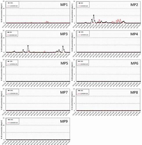
Figure 15. Time series of the 10-minute mean air concentrations of ⁸⁵Kr at each MP from 0600 JST to 1130 JST on 18 June 2008

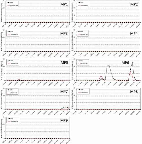
For the two cases, the MP positions where the mean concentrations were significantly detected were matched between the MP and LES data. Thus, the direction of plume transportation was accurately simulated.

4.3. Evaluation of dose-calculation module in LOHDIM-LES

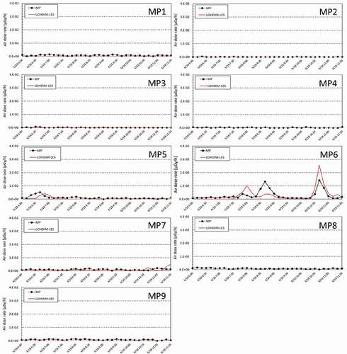
Figures 16 and 17 show time series of the air dose rates produced by ⁸⁵Kr in the air for the two simulation cases. Here, the air kerma free-in-air rates calculated by the SIBYL module from the LES 10-minute mean air concentrations were compared with the MP data of the air absorbed dose rates because both parameters are substantially equivalent for external gamma-ray exposures in the environment. The background values at each MP were assumed to be time-averaged values during the period that time variations of the air dose rates were not significantly observed, and those were excluded from the MP data. For case 1, the MP data demonstrated an intermittent increase in the air dose rates at MP2. These rates frequently showed higher peaks at MP3 than those at MP2. Therefore, the main part of the plume was transported above MP3. These time variation patterns at the different MPs were simulated well by the dose calculation method. For case 2, the MP data slightly increased at MP5 from 0610 JST to 0700 JST and showed two sharp, high peaks at MP6 from 0840 JST and 1040 JST. Thus, the main part of the plume was transported above MP5 and then above MP6 due to the change in the mean wind direction. The calculated data also showed a gentle peak at MP5 and sharp, high peaks at MP6. Despite the differences in the detection timing between the MP and calculated data for the two simulation periods, the time variation patterns and the magnitude of the fluctuations of the air dose rates were similar to the MP data. This was because the air dose rates at each stationary point was determined by the sum of the rates from the three-dimensional ⁸⁵Kr distributions, as stated by Abe et al. [25].

Figure 16. Time series of the air dose rate at each MP from 0900 JST to 1900 JST on 17 June 2008

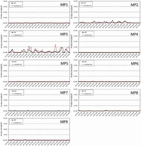
Figure 17. Time series of the air dose rate at each MP from 0600 JST to 1130 JST on 18 June 2008

Figure 18 shows a scatter plot of the air dose rates obtained at the MPs where the main part of the plume was transported for each simulation case. Here, FAC2 and FAC5, whose values are within 0.5–2.0 and 0.2–5.0, is the ratio of the calculated data to the MP data. From this definition, the best results have a value of 1.0. The air dose rate data for the scatter plot were extracted from data exceeding 5% of the maximum value during the simulation period, according to the definition proposed by Harms et al. [26]. The FAC2 and FAC5 of the air dose rates were 30% and 64%, respectively. Various methodologies for evaluating the performance of local-scale atmospheric dispersion models have been investigated. For example, Chang and Hanna [27], Hanna et al. [28], and Hanna and Chang [29] suggested that a good model should have FAC2 $\ge$ 50% for rural areas and FAC2 $\ge$ 30% for urban areas; these values were determined from a large number of model evaluation exercises during field experiments. However, these guidelines are only based on mean concentrations collected from several realizations in a dataset.

Figure 18. Scatter plot of the air dose rate. The solid and dashed lines indicate the perfect and FAC2 lines, respectively

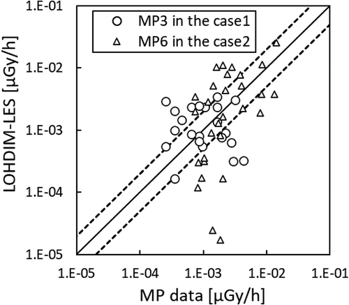
At present, there is no universal definition of acceptable criteria for air dose rates. It is difficult to fully evaluate the performance of local-scale atmospheric dispersion simulation in combination with a dose calculation method. Our model performance in air dose-rate estimation was comparable with acceptance values for mean concentrations in complex surface geometries, such as urban areas. Hence, the spatial distribution patterns of the air dose rates were simulated well. LOHDIM-LES equipped with a calculation method that uses dose-response matrices can reasonably estimate air dose rates over heterogeneous surface geometries covered with individual buildings and structures at the local-scale. However, the target radionuclide used for this model validation study was a non-depositing gas of ⁸⁵Kr as mentioned in the Section 3.1 and the plume rise formulation used here was also only one among the many proposed formulations. These are the major uncertainties in estimating air concentrations, surface depositions, and air dose rates. Sensitivity analysis is needed to examine these effects in future work.

5. Conclusion

We incorporated the dose-calculation module SIBYL into LOHDIM-LES and examined the model’s validity by applying it to the plume dispersion of radioactive materials released from a real nuclear facility. First, we verified the dose calculation method using dose-response and dose-attenuation matrices by comparing its results with the Monte-Carlo based three-dimensional radiation transport simulations by PHITS for the air dose rates produced by a radioactive plume and dry deposition in a regular array of cubic buildings. The results showed that the air dose rates were successfully simulated by LOHDIM-LES considering building shielding effects.

Then, we applied LOHDIM-LES integrated with the SIBYL module to the dose estimation of the radioactive plume dispersion in the nuclear facility. We then compared the model’s findings with the actual air dose rates produced by the 10-minute mean air concentrations of ⁸⁵Kr at the MPs in the vicinity of the facility. The time variation patterns and the magnitude of the fluctuations of the calculated air dose rates were generally similar to the MP data. A scatter plot was made for the air dose rates obtained at the MP where the main part of the plume was transported. It showed FAC2 and FAC5 values of 30% and 64%, respectively. Therefore, our model’s performance in air dose rate estimation satisfied the same acceptance criteria as those of mean concentrations for complex surface geometries. Comparisons with data measured at several MPs indicated that the spatial distribution patterns of the air dose rates were reasonably reproduced by our model. Given these validation results coupled with the verification results obtained using PHITS calculations, we concluded that LOHDIM-LES equipped with the calculation method using dose-response matrices can reasonably estimate air dose rates in consideration of the shielding effects of individual buildings and structures.

The completed version of LOHDIM-LES has a broad utility and offers superior performance in 1) simulating turbulent flows, plume dispersion, and dry deposition and 2) estimating the air dose rates of radionuclides from air concentrations and surface deposition in consideration of the influence of individual buildings and structures under realistic meteorological conditions. Although further improvement is needed in terms of high-speed computation to substantially reduce the model’s calculation time for its application in emergency response, LOHDIM–LES is promising for the safety assessment of nuclear facilities as an alternative to wind tunnel experiments and detailed pre/postanalyzes of the local-scale plume dispersion in nuclear accidents.

For example, experimental results are used only to derive the effective stack height, which is applied for long-term assessment using a Gaussian plume model. This approach has limited availability for these applications because wind tunnel testing is very expensive and time-consuming. Furthermore, such a simple model does not fully represent the turbulent effects of individual buildings on plume dispersion. In control room habitability assessment at nuclear power plants, adequate radiation protection is needed to allow access to and occupancy of a control room under accident conditions without personnel receiving radiation exposures in excess of specified values [30]. In case of terrorist attacks in urban central districts that use radiological materials, it would be necessary to estimate dose exposures for the general public and emergency exposure periods for first responders. In such situations, LOHDIM-LES could help accurately calculate dose consequences in consideration of inhomogeneous distributions of radioactive materials induced by individual buildings and structures.

We also plan to apply LOHDIM-LES to elucidate the dispersion processes of radionuclides in the vicinity of the Fukushima Daiichi Nuclear Power Plant, where only air dose rate data are available, during the early stage of the accident. Furthermore, the process-based and well-validated LOHDIM-LES can be used as a reference model to develop simple and quick models for emergency response or to improve the parameterization of turbulent diffusion and surface deposition processes for larger-scale dispersion models, such as WSPEEDI.

Acknowledgments

The authors thank the JNFL for providing the measurement data of the meteorological observation, release rate, air concentrations of ⁸⁵Kr, and air dose rates. The LESs were performed on the ICEX at Japan Atomic Energy Agency.

Disclosure statement

No potential conflict of interest was reported by the authors.

Appendix A.

Governing equations

The governing equations of LOHDIM-LES are the filtered continuity equation, incompressible Navier–Stokes equation in Boussinesq-approximated form, and the transport equations for potential temperature and material concentration.

(10) $\frac{\mathrm{\partial }{\bar{\mathrm{u}}}_i}{\mathrm{\partial }{x}_i}=0$(10)

(11) $\frac{\mathrm{\partial }{\bar{\mathrm{u}}}_i}{\mathrm{\partial }t}+{\bar{\mathrm{u}}}_j\frac{\mathrm{\partial }{\bar{\mathrm{u}}}_i}{\mathrm{\partial }{x}_j}=-\frac{1}{\rho }\frac{\mathrm{\partial }\bar{\mathrm{p}}}{\mathrm{\partial }{x}_j}-\frac{\mathrm{\partial }}{\mathrm{\partial }{x}_j}{\tau }_{ij}+g\frac{\bar{\theta }-\bar{\theta }}{{\theta }_0}{\delta }_{i3}-F_i$(11)

(12) $\frac{\mathrm{\partial }\bar{\theta }}{\mathrm{\partial }t}+{\bar{\mathrm{u}}}_j\frac{\mathrm{\partial }\bar{\theta }}{\mathrm{\partial }{x}_j}=-\frac{\mathrm{\partial }{q}_j}{\mathrm{\partial }{x}_j}$(12)

(13) $\frac{\mathrm{\partial }\bar{\mathrm{c}}}{\mathrm{\partial }t}+{\bar{\mathrm{u}}}_j\frac{\mathrm{\partial }\bar{\mathrm{c}}}{\mathrm{\partial }{x}_j}=-\frac{\mathrm{\partial }{s}_j}{\mathrm{\partial }{x}_j}$(13)

where $u_i$, $p$, $\rho$, ${\tau }_{ij}$, $g$, $\theta$, ${\theta }_0$, $F_i$, $q_j$, $c$, and $s_j$ are the wind velocity, pressure, air density, subgrid-scale Reynolds stress, gravity acceleration, temperature, reference temperature, external force, subgrid-scale heat flux, concentration, and subgrid-scale concentration flux, respectively. Subscripts $i$ and $j$ stand for coordinates (streamwise direction, $x_1=x;$ spanwise, $x_2=y;$ vertical, $x_3=z;$). Overbars $\left(\stackrel{‾}{}\right)$ indicate that the variable is spatially filtered. ${\delta }_{ij}$ is the Kronecker delta (${\delta }_{ij}$ = 1 for $i=j$; ${\delta }_{ij}$ = 0 otherwise). The angle brackets represent a horizontal average.

The subgrid-scale turbulent effect is represented by the standard Smagorinsky model [17] with a constant value of 0.1. The subgrid-scale scalar flux is also parameterized by an eddy viscosity model as follows:

(14) ${\tau }_{ij}=-2{\nu }_{SGS}{\bar{\mathrm{S}}}_{ij}$(14)

(15) ${\nu }_{SGS}={\left(C_s\bar{\mathrm{\Delta }}\right)}^2{\left(2{\bar{\mathrm{S}}}_{ij}{\bar{\mathrm{S}}}_{ij}\right)}^2$(15)

(16) ${\bar{\mathrm{S}}}_{ij}=\frac{1}{2}\left(\frac{\mathrm{\partial }{\bar{\mathrm{u}}}_i}{\mathrm{\partial }{x}_j}+\frac{\mathrm{\partial }{\bar{\mathrm{u}}}_j}{\mathrm{\partial }{x}_i}\right)$(16)

(17) $\bar{\mathrm{\Delta }}={\left({\bar{\mathrm{\Delta }}}_x{\bar{\mathrm{\Delta }}}_y{\bar{\mathrm{\Delta }}}_z\right)}^{\frac{1}{3}}$(17)

(18) $q_j=-\frac{{\nu }_{SGS}}{P{r}_{SGS}}\frac{\mathrm{\partial }\bar{\theta }}{\mathrm{\partial }{x}_j}$(18)

(19) $s_j=-\frac{{\nu }_{SGS}}{S{c}_{SGS}}\frac{\mathrm{\partial }\bar{\mathrm{c}}}{\mathrm{\partial }{x}_j}$(19)

where ${\nu }_{SGS}$, $C_s$, ${\bar{\mathrm{S}}}_{ij}$, $\bar{\mathrm{\Delta }}$, $P{r}_{SGS}$, and $S{c}_{SGS}$ are the eddy viscosity coefficient, model constant of the flow field, strain-rate tensor, grid-filter width, turbulent Prandtl, and Schmidt numbers, respectively.

The external force term $F_i$ is composed of the following forcing terms:

(20) $F_i=f_{i\mathrm{\_}ibm}+f_{i\mathrm{\_}canopy}$(20)

(21) $f_{i\mathrm{\_}ibm}=\alpha \underset{0}{\overset{t}{\int }}{\bar{\mathrm{u}}}_i\left(x,y,z,t^{\prime }\right)dt{ }^{\mathrm{\prime }}+\beta {\bar{\mathrm{u}}}_i\left(x,y,z,t^{\prime }\right)$(21)

(22) $f_{i\mathrm{\_}canopy}=C_{d}a\left(z\right){\bar{\mathrm{u}}}_{i}U$(22)

where the building and terrain effects $\left(f_{i\mathrm{\_}ibm}\right)$ are calculated by the immersed boundary method, which was proposed by Goldstein et al. [18]. $\alpha$ and $\beta$ are negative constants. The forest canopy effect $\left(f_{i\mathrm{\_}canopy}\right)$ is represented by the drag force, which consists of the drag coefficient $\left(C_d\right)$; the frontal area density of the vegetation $\left(a\left(z\right)\right)$; wind velocities; and wind speed magnitude $\left(U\right)$.

The ground surface conditions for the flow and temperature fields are represented as follows:

(23) ${\tau }_{i3\mathrm{\_}wall}=-{\left(\frac{\kappa {\bar{\mathrm{u}}}_i}{ln\left(z/z_0\right)-{\psi }_M}\right)}^2$(23)

(24) $q_{3\mathrm{\_}wall}=\frac{u_{\ast }\kappa \left({\theta }_s-\bar{\theta }\right)}{ln\left(z/z_0\right)-{\psi }_H}$(24)

where ${\tau }_{i3\mathrm{\_}wall}$, $\kappa$, $z_0$, $q_{3\mathrm{\_}wall}$, $u_{\ast }$, and ${\theta }_s$ are the instantaneous wall stress, von Karman constant, roughness length, surface heat flux, friction velocity, and surface temperature, respectively. ${\psi }_M$ and ${\psi }_H$ are the stability corrections for momentum and heat, respectively. ${\tau }_{i3\mathrm{\_}wall}$ is represented by Monin-Obukhov similarity theory [31], and $q_{3\mathrm{\_}wall}$ is computed in a similar manner.

When dry deposition is considered, the decay rates of concentrations are represented using dry deposition velocity as follows [20,32]:

(25) $\frac{\mathrm{\partial }\bar{\mathrm{c}}}{\mathrm{\partial }t}=-\frac{V_d}{{\bar{\mathrm{\Delta }}}_{i\mathrm{\_}wall}}{\bar{\mathrm{c}}}_{wall}$(25)

where ${\bar{\mathrm{\Delta }}}_{i\mathrm{\_}wall}$ is the grid spacing in a cell of ground and building surfaces where radionuclides are deposited in the i-direction.

Appendix B.

LES turbulent inflow conditions

The following turbulence generation method, formed by a combination of the recycling method [33] and the Langevin-type equation [34,35], was used to efficiently generate TBL flows by a short development section.

(26) $u_{infl}\left(y,z,t\right)=U_{infl}\left(z\right)+\theta \left(z\right)\times \left\{{u{ }^{\mathrm{\prime }}}_{recy}\left(y,z,t\right)+{u{ }^{\mathrm{\prime }}}_{lang}\left(y,z,t\right)\right\}$(26)

(27) ${u{ }^{\mathrm{\prime }}}_{recy}\left(y,z,t\right)=u_{recy}\left(y,z,t\right)-\left[u_{recy}\left(z,t\right)\right]$(27)

(28) $u{\prime }_{lang}\left(y,z,t\right)=\left(1-\frac{\mathrm{\Delta }t}{T_u\left(z\right)}\right)u{\prime }_{lang}\left(y,z,t-\mathrm{\Delta }t\right)+{\sigma }_u\left(z\right){\left(\frac{2\mathrm{\Delta }t}{T_u\left(z\right)}\right)}^{1/2}\xi$(28)

where $u_{infl}$ and $U_{infl}$ are the instantaneous and mean streamwise $\left(x\right)$ wind components, respectively, at the inflow boundaries. $y$, $z$, and $t$ are the spanwise direction, vertical direction, and time, respectively. $U_{infl}$ is usually given by a representative wind velocity and by MM or OBS data for ideal and realistic meteorological conditions, respectively. $u_{recy}^{\prime }$ and $u_{lang}^{\prime }$ indicate the turbulent fluctuating components extracted at a downstream position by the recycling method and generated by the Langevin-type equation, respectively. The recycling station is set to the downstream position of 500 m from the inflow boundary. $\left[u\right]$ is the horizontally averaged wind. $\theta \left(z\right)$ is a damping function that controls the development of the simulated TBL. ${\sigma }_u\left(z\right)$, $T_u\left(z\right)$, and $\xi$ are the standard deviation of wind velocity, the time integral scale, and a random number, respectively. ${\sigma }_u\left(z\right)$ and $T_u\left(z\right)$ were obtained from the Engineering Science Data Unit (ESDU) 85,020 data, which recommend vertical profiles of turbulence intensities for each wind component and their relationship depending on surface roughness [36]. Findings showed that the basic TBL flows under varying mean wind directions were reasonably reproduced by this turbulence generation method [37].

Since mean wind directions often vary due to changes in meteorological conditions, the vertical planes at the inflow and outflow boundaries are set to be automatically prescribed depending on them. At the upper boundary, a free-slip condition for the horizontal velocity components and a zero-speed condition for the vertical velocity component are imposed. At the outlet boundary, a free-slip condition is applied for each component of wind velocity. At the bottom surface, Monin-Obukhov similarity theory is applied as mentioned in Appendix A. For the concentration field, a zero-gradient condition is imposed at all boundaries.

References

- Nagai H, Chino M, Yamazawa H. Development of scheme for predicting atmospheric dispersion of radionuclides during nuclear emergency by using atmospheric dynamic model. , Journal of the Atomic Energy Society of Japan / Atomic Energy Society of Japan. 1999;41(7):777–785. in Japanese. .
- Terada H, Nagai H, Furuno A, et al. Development of worldwide version of system for prediction of environmental emergency dose information: WSPEEDI 2nd Version. Trans At Energy Soc Jpn. 2008;7(3):257–267.
- Sada K, Komiyama S, Michioka T, et al. Numerical model for atmospheric diffusion analysis and evaluation of effective dose for safety analysis. Transactions of the Atomic Energy Society of Japan. 2009;8(2):184–196. in Japanese. .
- Nakayama H, Nagai H. Development of local-scale high-resolution atmospheric dispersion model using Large-Eddy simulation part 1: turbulent flow and plume dispersion over a flat terrain. Journal of Nuclear Science and Technology. 2009;46(12):1170–1177.
- Nakayama H, Nagai H. Development of local-scale high-resolution atmospheric dispersion model using large-eddy simulation part 2: turbulent flow and plume dispersion around a cubical building. Journal of Nuclear Science and Technology. 2011;48(3):374–383.
- Nakayama H, Nagai H. Large-Eddy Simulation on turbulent flow and plume dispersion over a 2-dimensional hill. Advances in Science and Research. 2010;4(1):71–76.
- Nakayama H, Jurcakova K, Nagai H. Development of local-scale high-resolution atmospheric dispersion model using large-eddy simulation. Part 3: turbulent flow and plume dispersion in building arrays. Journal of Nuclear Science and Technology. 2013;50(5):503–519.
- Nakayama H, Leitl B, Harms F, et al. Development of local-scale high-resolution atmospheric dispersion model using large-eddy simulation. Part 4: turbulent flows and plume dispersion in an actual urban area. Journal of Nuclear Science and Technology. 2014;51(5):626–638.
- Nakayama H, Nagai H. Local-scale High-resolution atmospheric dispersion model using large-eddy simulation: LOHDIM-LES, JAEA-Data/Code, 2015–2026.
- Ono H, Takimoto H, Sato A, et al. Development of a numerical model for predicting the atmospheric dispersion of hydrogen-sulfide emitted from geothermal power plants. Trans At Energy Soc Jpn. 2017;52: 19–29. in Japanese.
- Nakayama H, Takemi T, Nagai H. Large-eddy simulation of urban boundary-layer flows by generating turbulent inflows from mesoscale meteorological simulations. Atmospheric Science Letters. 2012;13(3):180–186.
- Nakayama H, Takemi T, Nagai H. Development of LO cal-scale High-resolution atmospheric DI spersion Model using Large-Eddy Simulation. Part 5: detailed simulation of turbulent flows and plume dispersion in an actual urban area under real meteorological conditions. Journal of Nuclear Science and Technology. 2016;53(6):887–908.
- Sato T, Iwamoto Y, Hashimoto S, et al. Features of particle and heavy ion transport code system (PHITS) version 3.02. Journal of Nuclear Science and Technology. 2018;55(6):684–690.
- Satoh D, Kojima K, Oizumi A, et al. Development of a calculation system for the estimation of decontamination effects. Journal of Nuclear Science and Technology. 2014;51(5):656–670.
- Satoh D, Nakayama H, Furuta T, et al. Simulation code for estimating external gamma-ray doses from a radioactive plume and contaminated ground using a local-scale atmospheric dispersion model. Plos One. 2021. DOI:https://doi.org/10.1371/journal.pone.0245932.g011
- Harlow F, Welch JE. Numerical Calculation of Time-Dependent Viscous Incompressible Flow of Fluid with Free Surface. Physics of Fluids. 1965;8(12):2182–2189.
- Smagorinsky J. General circulation experiments with the primitive equations. Mon Weather Rev. 1963;91(3):99–164.
- Goldstein D, Handler R, Sirovich L. Modeling a no-slip flow boundary with an external force field. Journal of Computational Physics. 1993;105(2):354–366.
- Nuclear Safety Commission of Japan. Meteorological guide for safety analysis of nuclear power plant reactor. Tokyo: Nuclear Safety Commission of Japan; 1982. in Japanese.
- Pugh TAM, MacKenzie AR, Whyatt JD, et al. Effectiveness of green infrastructure for improvement of air quality in urban street canyons. Environmental Science & Technology. 2012;46(14):7692–7699.
- Moeng H, Sullivan P. A comparison of shear- and buoyancy-driven planetary boundary layer flows. J Atmos Sci. 1994;51(7):999–1022.
- Okamoto S, Okanishi S, Hiroh A. Comparison and evaluation of plume rise formulas. J Japan Society Air Pollution. 1977;12:456–465.
- Brummage KG. The calculation of atmospheric dispersion from a stack, Stichhting CONCAWE. The Hague, The Netherlands: 57; August 1966.
- Davidson M, Mylne K, Jones C, et al. Plume dispersion through large groups of obstacles—A field investigation. Atmospheric Environment. 1995;29(22):3245–3256.
- Abe K, Iyogi T, Kawabata H, et al. Estimation of 85Kr dispersion from the spent nuclear fuel reprocessing plant in Rokkasho, Japan, using an atmospheric dispersion model. Radiation Protection Dosimetry. 2015;167(1–3):331–335.
- Harms F, Leitl B, Schatzmann M, et al. Validating LES-based flow and dispersion models. Journal of Wind Engineering and Industrial Aerodynamics. 2011;99(4):289–295.
- Chang JC, Hanna SR. Air quality model performance evaluation. Meteorol Atmos Phy. 2004;87(1–3):167–196.
- Hanna SR, Hansen OR, Dharmavaram S. FLACS CFD air quality model performance evaluation with Kit Fox, MUST, Prairie Grass, and EMU observations. Atmos Environ. 2004;38(28):4675–4687.
- Hanna SR, Chang JC. Acceptance criteria for urban dispersion model evaluation. Meteorol Atmos Phys. 2012;116(3–4):133–146.
- U.S. Nuclear Regulatory Commission, 2003: Control room habitability at light-water nuclear power reactors, Regulatory guide 1.196.
- Monin A, Obukhov M. Basic laws of turbulent mixing in the ground layer of the atmosphere. Tr Akad Nauk SSSR Geophiz Inst. 1954;24:163–187.
- Jeanjean APR, Monks PS, Leigh RJ. Modelling the effectiveness of urban trees and grass on PM2.5 reduction via dispersion and deposition at a city scale. Atmospheric Environment. 2016;147:1–10.
- Kataoka H, Mizuno M. Numerical flow computation around aeroelastic 3D square cylinder using inflow turbulence. Wind and Structures. 2002;5(2_3_4):379–392.
- Hanna SR, Tehranian S, Carissimo B, et al. Comparisons of model simulations with observations of mean flow and turbulence within simple obstacle arrays. Atmospheric Environment. 2002;36(32):5067–5079.
- Tolias IC, Koutsourakis N, Hertwig D, et al. Large Eddy Simulation study on the structure of turbulent flow in a complex city. Journal of Wind Engineering and Industrial Aerodynamics. 2018;177:101–116.
- Engineering Science Data Unit, 1985: Characteristics of atmospheric turbulence near the ground part2 single point data for strong winds (neutral atmosphere), ESDU Item, 85020.
- Nakayama H, Takemi T. Large-eddy simulation studies for predicting plume concentrations around nuclear facilities using an overlapping technique. International Journal of Environment and Pollution. 2018;64(1/2/3):125–144.