Quantitative visualization of a radioactive plume with harmonizing gamma-ray imaging spectrometry and real-time atmospheric dispersion simulation based on 3D wind observation

ABSTRACT

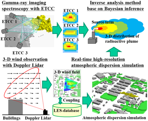
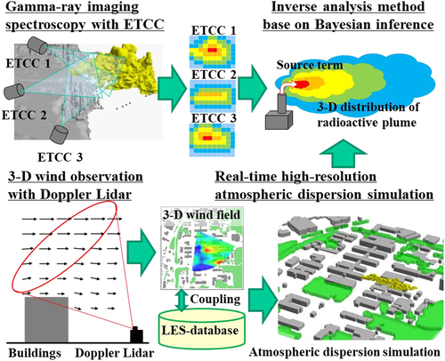
To propose a novel monitoring method for the quantitative visualization of 3D distribution of a radioactive plume in the vicinity of release point and source term estimation of released radionuclides, the feasibility of its analysis method is demonstrated by preliminary test. The proposed method is the combination of gamma-ray imaging spectroscopy with the electron tracking Compton camera (ETCC) and real-time high-resolution atmospheric dispersion simulation based on 3D wind observation with Doppler lidar. ETCC can acquire the angle distribution images of direct gamma-ray from a specific radionuclide in a target radioactive plume by quantitatively capturing gamma-ray incidence angles and spectrum distributions. The 3D distribution of each radionuclide in the radioactive plume is inversely reconstructed from direct gamma-ray images of each radionuclide by several ETCCs located around the target by harmonizing with the air concentration distribution pattern of the plume predicted by real-time atmospheric dispersion simulation. A prototype of the analysis method was developed, showing a sufficient performance in several test cases using hypothetical data generated by numerical simulations of atmospheric dispersion and radiation transport. The proposed method is expected to become an innovative monitoring framework for nuclear emergency.

GRAPHICAL ABSTRACT

KEYWORDS:

• Quantitative visualization of radioactive plume
• source term
• radiation imaging
• atmospheric dispersion simulation
• wind observation with Doppler lidar

1. Introduction

In case of a nuclear accident with substantial discharge of radioactive materials into the atmosphere, for example, the Chernobyl nuclear reactor accident in 1986 and the Fukushima Daiichi Nuclear Power Station (FDNPS) accident in 2011, grasping the spatiotemporal behavior of released radioactive materials in the environment is essential for emergency countermeasures, such as evacuation planning and impact assessments. Besides the environmental monitoring around nuclear sites, an atmospheric dispersion simulation of radioactive materials is a useful tool for these countermeasures in providing spatiotemporal compensation of monitoring data and future projection. For this purpose, a computer simulation system coupled with monitoring network, i.e. the system for prediction of environmental emergency dose information (SPEEDI), was developed by the Japan Atomic Energy Research Institute (now Japan Atomic Energy Agency, JAEA) [1] and operated by the Nuclear Safety Technology Center as an emergency response system for domestic nuclear accident in Japan. However, while simulation results by SPEEDI were utilized to select monitoring points during the early phase of the FDNPS accident, they were not used in the decision-making for evacuation planning as the decision-maker judged the prediction results as unreliable due to uncertainties in the model simulations [2]. The uncertainty was mainly attributed to the lack of necessary input information for SPEEDI simulations, namely, the source term of released radioactive materials, which was neither provided by another emergency response system (Emergency Response Support System, ERSS) nor stack monitors at FDNPS as indicated in the emergency response manual due to the power outage [2]. It should be further pointed out that the source term with complex release conditions and temporal profile in the FDNPS accident would not be provided even if ERSS and the stack monitors were active.

On the other hand, SPEEDI and the Worldwide version of SPEEDI (WSPEEDI) [3] developed by JAEA were effectively utilized in the impact assessment. JAEA has been working to estimate the source term by coupling atmospheric dispersion simulations of these systems with environmental monitoring data [4–11]. The WSPEEDI simulation using the estimated source term successfully reproduced the air dose rates and air concentrations and deposition patterns of radionuclides measured after the FDNPS accident. It also revealed how the radioactive materials were transported and deposited on and around the main island of Japan after the incident. The simulation results by the latest study [11] were also used for comprehensive dose assessment by coupling with behavioral patterns of evacuees from the FDNPS accident by a project team in Japan [12] and the United Nations Scientific Committee on the Effects of Atomic Radiation (UNSCEAR) [13]. Based on these experiences, JAEA also developed a new calculation method of WSPEEDI (WSPEEDI-DB) [14], which can immediately obtain prediction results by applying the source term to the database of dispersion calculation results prepared in advance. Furthermore, the database generated by WSPEEDI-DB was utilized to develop a method to estimate uncertainty in forecasted plume directions [15, 16] and a real-time application method of WSPEEDI-DB for the reconstruction of the source term and multi-scale atmospheric dispersion processes [17]. These WSPEEDI-DB functions are expected to provide useful information for emergency countermeasures. However, the source term for the FDNPS accident has not been fully reconstructed by these studies due to the lack of monitoring data especially at the vicinity of FDNPS and information about release conditions, such as release pattern (stack release, leakage from building, explosion, etc.), timing of release phase change, radionuclides composition, and physical and chemical forms of radionuclides.

The enhancement of monitoring networks around nuclear facilities has been carried out after the FDNPS accident to grasp the spatiotemporal distribution of radioactive materials discharged into the environment during a nuclear accident. In the monitoring network, monitoring posts for air dose rate measurement are densely distributed (about 5-km resolution) within the urgent protective action planning zone, i.e. 30-km radius of a nuclear facility based on the guideline by the Nuclear Regulation Authority [18]. Although a radioactive plume passage can be captured by air dose rate data with the monitoring posts network, air concentrations of radionuclides in the plume cannot be obtained. The measured data of air dose rate from radionuclides deposited on the ground surface (ground shine) after the plume passage are used for decision-making of evacuation. Air concentrations of radionuclides are also measured by dust monitors with coarser mesh than the monitoring posts network. However, it takes long time (hours to days) to derive air concentration data from dust samples. Therefore, these air concentration data are not used for grasping the radioactive plume condition for evacuation planning but for dose assessment in the post analysis. To increase the effectiveness of the monitoring posts network for grasping the quantitative features of radioactive plume, it is necessary to develop and install a method to determine the composition of major radionuclides into the monitoring posts network, such as the analysis of pulse height distributions measured with NaI(Tl) scintillation detectors [19–21]. However, these conventional monitoring methods have the limitation in capturing the 3D structure of radioactive plume due to the point data at the ground surface.

A gamma-ray imaging is expected to be an effective method to capture the 3D structure of radioactive plume. Many gamma cameras have been developed to produce imaging observations to help decontamination of FDNPS, based on a Compton camera [22–26] and a pinhole camera [27]. Although these gamma cameras successfully detected hot spots by generating gamma-ray intensity distribution images for contaminated surfaces of reactor buildings of FDNPS, none of them showed any quantitative radiation images. Their performances were far from the imaging spectroscopy for identifying a specific radionuclide. Compton cameras have an intrinsic difficulty in imaging spectroscopy due to its blurred image with large half intensity width of the point spread function (PSF) [28, 29]. On the other hand, pinhole cameras, which keep the directional information of each incoming gamma-ray, are capable of imaging spectroscopy. However, the effective area of PHC is seriously small and has low sensitivity to measure a radioactive plume.

The electron tracking Compton camera (ETCC) has been developed to attain the gamma-ray imaging spectroscopy [28, 29]. ETCC was originally developed to observe gamma-ray from celestial objects in MeV astronomy [30] but has been applied in wider fields, including medical imaging [31] and environmental monitoring [32, 33]. It can provide the brightness distribution of gamma-ray with high-resolution of PSF by resolving the Compton process completely with the additional information from a 3D recoil electron-tracking measurement [29]. It is expected that the gamma-ray spectroscopy with ETCC can acquire the angle distribution images of direct gamma-ray from a specific radionuclide in a target radioactive plume, and the 3D distribution of each radionuclide in the radioactive plume is inversely reconstructed from direct gamma-ray images by several ETCCs located around the target.

In the present study, a novel monitoring method utilizing ETCC is proposed, which can quantitatively visualize a radioactive plume just after the accidental discharge from a nuclear facility. Here the quantitative visualization means the reconstruction of digital model of radioactive plume with 3D air concentration distributions of radionuclides, which can also provide the source term of each radionuclide. For the inverse reconstruction of 3D air concentration distribution of a radionuclide from gamma-ray imaging spectroscopy with ETCC, additional information is necessary to cope with the rapidly changing plume pattern due to the atmospheric dispersion. Therefore, the harmonization of the gamma-ray imaging spectroscopy by ETCC with atmospheric dispersion simulation based on 3D wind observation is considered. The feasibility of the inverse analysis in the proposed method is demonstrated by preliminary testing using hypothetical data generated by numerical simulations of atmospheric dispersion and radiation transport.

2. Materials and method

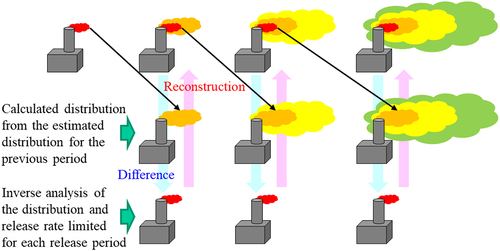
The proposed monitoring method for the quantitative visualization of a radioactive plume consists of the gamma-ray imaging spectroscopy with ETCC, real-time high-resolution atmospheric dispersion simulation based on 3D wind observation with Doppler lidar [34], and inverse analysis method to reconstruct the radioactive plume quantitatively from gamma-ray image and atmospheric dispersion simulation data (Figure 1). Subsections 2.1, 2.2, and 2.3 present the gamma-ray imaging spectroscopy, real-time high-resolution atmospheric dispersion simulation, and inverse analysis method, respectively. Subsection 2.4 describes the experimental setup of preliminary tests to demonstrate the feasibility of the proposed method.

Figure 1. Proposed monitoring method for the quantitative visualization of a radioactive plume.

2.1. Gamma-ray imaging spectroscopy

This section describes the basis of gamma-ray imaging spectroscopy with ETCC and the method of its application to the quantitative visualization of a radioactive plume. The conventional Compton camera uses two layers of gamma-ray detectors, and the incident gamma-ray angle is determined from the relationship between the positions of scattering the incident gamma-ray by the front detector layer and receiving the scattered gamma-ray by the rear detector layer. Since the incident gamma-ray angle cannot be uniquely determined for each gamma-ray incident event due to the lack of information about the scattering process, it is necessary to be specified by superposition of results from many incident events. This is the reason that Compton cameras have blurred image with large half intensity width of PSF and cannot provide the quantitative radiation images. In contrast to the conventional Compton camera, ETCC uses a gaseous time projection chamber (TPC) for the front detector, and the incident gamma-ray angle is determined with high-resolution of PSF for each gamma-ray incident event by resolving the Compton process completely with the additional information from a 3D recoil electron-tracking measurement in TPC, as shown in Figure 2 [29]. It also provides the quantitative radiation images with energy spectrum. Therefore, ETCC can acquire the angle distribution images of direct gamma-ray from the distribution of a specific radionuclide.

Figure 2. Schematic view of ETCC and schematic explanation of difference in PSF between the conventional Compton camera and ETCC.

In the application to the quantitative visualization of a radioactive plume, several gamma-ray images are taken from different angles by ETCCs located around the target gamma-ray source, as shown in Figure 1. ETCC can take a gamma-ray image for the 120-degree angular area with PSF of currently 10 degrees and possibly 1 degree in the near future, which has much higher resolution than that of conventional Compton cameras with PSF of about 40 degrees (Figure 2). The energy resolution of the current ETCC using Ce-doped Gd₂SiO₅ (Ce:GSO) scintillators is 10% in full-width half maximum at 662 keV, which can be improved up to about 5% by using Ce-doped Gd₃(Al,Ga)₅O₁₂ (C:GAGG) scintillators [35]. The direct gamma-ray image from a specific radionuclide in the plume is derived by removing the background energy spectrum from the energy spectrum at the peak region of the target radionuclide [29]. The background energy of air-scattered gamma-ray including the influence of the contaminated background can be obtained from the angular areas of ETCC not viewing the plume. ETCC can detect the energy spectrum change within 1 min in case of the air dose rate change of 0.2 μSv h⁻¹ at the monitoring point [35]. This detection sensitivity is high enough to take the gamma-ray image from a radioactive plume within a few minutes, and the temporal changes in 3D distribution of each radionuclide in the plume can be captured for the FDNPS accident case. In this study, it is assumed that ETCC outputs the direct gamma-ray image for the angular area of 100 degrees × 100 degrees with resolution of 5 degrees every minute.

2.2. Real-time high-resolution atmospheric dispersion simulation

In the proposed method for the inverse reconstruction of 3D air concentration distribution of a radionuclide in the plume, the real-time high-resolution atmospheric dispersion simulation based on 3D wind observation with Doppler lidar [34] was used for the harmonization with the gamma-ray imaging spectroscopy, as shown in Figure 1. Simulations of LOcal-scale High-resolution atmospheric DIspersion Model using Large-Eddy Simulation (LOHDIM-LES) developed by JAEA [36–42] were utilized to generate high-resolution wind and turbulence fields for detailed dispersion simulations. It provides detailed computed data of wind velocities, temperatures, air concentrations, and dry deposition amounts at the ground and/or building surfaces in the vicinity of nuclear facilities and central urban districts under ideal or realistic meteorological conditions, which were well validated against wind tunnel and field experiments [42]. LOHDIM-LES is a computational fluid dynamics model, and the governing equations are the filtered continuity equation, the Navier–Stokes equation in Boussinesq approximation form, and the transport equations of heat and mass. The Smagorinsky model [43] represents the sub-grid scale turbulent effect. The sub-grid scale scalar fluxes are also parameterized by an eddy viscosity model. Buildings and structures are explicitly represented by the use of a digital surface model dataset. The turbulent effects of buildings are represented by the immersed boundary method [44]. Since the computational cost for LOHDIM-LES simulation is extremely high, it cannot be used for the real-time analysis. Instead, LOHDIM-LES simulations are carried out beforehand for various kinds of meteorological conditions to construct a database of high-resolution wind and turbulence fields considering building effects in the target analysis area (LES database) with horizontal grid resolution usually less than 10 m. The LES database contains 3D distributions of mean wind speed and turbulence standard deviation for wind directions (typically 36 different mean wind directions at class interval of 10 degrees) and atmospheric thermal stability conditions (stable, neutral, and unstable). The wind speed is not classified in the LES database because wind speeds at model grids are scaled to observed wind velocities as described below.

The real-time high-resolution atmospheric dispersion simulation is performed for the wind and turbulence fields generated by coupling the 3D wind observation with Doppler lidar and pre-calculated LES database. These wind field data are combined based on the boundary layer flow structure with three layers, namely, the building canopy layer, the roughness sublayer, and the inertial sublayer, as shown in Figure 3. In the building canopy layer, the flow patterns are directly determined by building arrangements and show a strong three-dimensionality caused by impinging, separated, and recirculating flows, which can be reproduced by LOHDIM-LES. The depth of the roughness sublayer ranges up to 2–5 times the height of the buildings [45]. In the inertial sublayer, the dynamic influence of the surface decreases with height, and the flows eventually readjust to the meteorological conditions, which can be captured by the Doppler lidar observation, as shown in Figure 3. The Doppler lidar used in this study includes both Plan Position Indicator (PPI) scans at arbitrary elevation angles and Range Height Indicator (RHI) scans at arbitrary azimuth angles with a few-minutes scan sequence. The horizontal and vertical components of the wind velocities are obtained at the maximum detection range of 10 km with a range resolution of dozens of meters in the radial direction. The laser beam is intensively directed toward the release point to obtain the 3D distribution of wind velocities inducing plume rise driven by inertia and buoyancy. Considering these characteristics, input data for the real-time high-resolution atmospheric dispersion simulation are constructed as follows. Firstly, 3D wind field by the Doppler lidar observation is directly interpolated to the model calculation grids in the inertial sublayer. Wind profiles derived from the LES database, which corresponds to the observed meteorological condition, are then given to the model grids in the roughness sublayer after being scaled to the observed wind at the lowest height of the inertial sublayer with the following equation:

(1) $U\left(x,y,z\right)=U_{LES}\left(x,y,z\right)\frac{U_{OBS}\left(x,y,h\left(x,y\right)\right)}{U_{LES}\left(x,y,h\left(x,y\right)\right)},$(1)

Figure 3. Typical structure of boundary layer flows over buildings and 3D wind field measurement by Doppler lidar.

where $U$, $U_{LES}$, and $U_{OBS}$ are the scaled wind velocities, the original wind velocities in the LES database, and observed ones interpolated to the model grids, respectively. $h\left(x,y\right)$ is the lowest height of the inertial sublayer at the grid point $\left(x,y\right)$. Turbulence standard deviations in the LES database are also normalized as follows:

(2) ${\sigma }_u\left(x,y,z\right)=\frac{{\sigma }_{u\mathrm{\_}LES}\left(x,y,z\right)}{U_{LES}\left(x,y,z\right)}\left(aU\left(x,y,z\right)+b\right)$(2)

(3) ${\sigma }_v\left(x,y,z\right)=\frac{{\sigma }_{v\mathrm{\_}LES}\left(x,y,z\right)}{{\sigma }_{u\mathrm{\_}LES}\left(x,y,z\right)}{\sigma }_u\left(x,y,z\right)$(3)

(4) ${\sigma }_w\left(x,y,z\right)=\frac{{\sigma }_{w\mathrm{\_}LES}\left(x,y,z\right)}{{\sigma }_{u\mathrm{\_}LES}\left(x,y,z\right)}{\sigma }_u\left(x,y,z\right)$(4)

where ${\sigma }_u$, ${\sigma }_v$, and ${\sigma }_w$ are the x-, y-, and z-components of the normalized turbulence standard deviation, respectively, and the subscript ‘LES’ indicates the values in the LES database. For the mean turbulence standard deviation, the constants of $a$ and $b$ are 0.75 and 3.8, respectively [46].

Using the high-resolution wind and turbulence fields generated above, the real-time high-resolution atmospheric dispersion simulation is conducted with a Lagrangian particle dispersion model [47]. The basic equations are as follows.

(5) $x_i\left(t+\mathrm{\Delta }t\right)=x_i\left(t\right)+u_{pi}\mathrm{\Delta }t$(5)

(6) $u_{pi}=U_i+u_i^{\prime }$(6)

(7) $u_i^{\prime }\left(t+\mathrm{\Delta }t\right)=\alpha u_i^{\prime }\left(t\right)+\beta {\sigma }_{ui}\xi +{\delta }_{i3}\left(1-\alpha \right)t_{Lxi}\frac{\mathrm{\partial }{\sigma }_{ui}^2}{\mathrm{\partial }{x}_i}$(7)

(8) $\alpha =exp(\frac{-\mathrm{\Delta }t}{t_{Lxi}})$(8)

(9) $\beta ={\left(1-{\alpha }^2\right)}^{1/2}$(9)

where $x_i$ is the particle position in the ith direction (east–west direction, i = 1; north–south direction, i = 2; vertical direction, i = 3), $u_{pi}$, $U_i$, $u_i^{\prime }$, and ${\sigma }_{ui}$ are particle velocity, mean wind velocity, turbulence velocity, and standard deviation of the velocity fluctuation, respectively, $\xi$ is a random number from a Gaussian distribution with zero mean and unit variance, $t_{Lxi}$ is the Lagrangian integral time, ${\delta }_{i3}$ is the Dirac delta function, $t$ and $\mathrm{\Delta }t$ are time and calculation time step interval, respectively. The concept of the turbulence diffusion part expressed by Equation (7)(7) $u_i^{\prime }\left(t+\mathrm{\Delta }t\right)=\alpha u_i^{\prime }\left(t\right)+\beta {\sigma }_{ui}\xi +{\delta }_{i3}\left(1-\alpha \right)t_{Lxi}\frac{\mathrm{\partial }{\sigma }_{ui}^2}{\mathrm{\partial }{x}_i}$(7) is as follows. The influence of the turbulence velocity on plume spreads mainly depends on the Lagrangian integral time and the standard deviation of the velocity fluctuations. Plume spreads become larger near the release point with increase in the velocity fluctuations while the influence is smaller with the downwind distance. On the other hand, there is no significant influence of the Lagrangian integral time on plume spreads near the release point while those become larger with the downwind distance.

2.3. Inverse analysis method

The 3D distribution of each radionuclide in the radioactive plume and source term of released radionuclides are inversely reconstructed from gamma-ray images by several ETCCs located around the target by harmonizing with the air concentration distribution pattern of the plume predicted by the real-time atmospheric dispersion simulation using unit release condition. In this analysis, a gamma-ray response function matrix is created in advance, as shown in Figure 4, to immediately calculate angular distribution of direct gamma-ray intensity incident on ETCC from the 3D distribution of each radionuclide in the atmosphere. The gamma-ray response function matrix contains a set of conversion factors to calculate the direct gamma-ray intensity incident on angular areas of ETCC (20 × 20 areas with a 5-degree resolution in the present study) from the radioactivity of each radionuclide in all 3D grid cells (nx × ny × nz) in the analysis domain. The conversion factor of direct gamma-ray intensity for a specific gamma-ray energy of each radionuclide is defined as the gamma-ray count rate at unit solid angle, time, and area of ETCC regarding unit radioactivity concentration of a grid cell (count str⁻¹ sec⁻¹ cm⁻² (Bq m⁻³)⁻¹). The gamma-ray count rate at each angular area of ETCC is calculated as follows. First, a huge number of particles assuming radionuclide are distributed randomly in a grid cell (3,000 particles per unit volume in this study). Then, the probability of a gamma-ray incident event at the ETCC from each particle is calculated by multiplying the incident rate determined by the geometric relationship between ETCC and the particle, the emission rate of the gamma-ray, and attenuation rate of gamma-ray in air based on the distance from the particle and ETCC and the attenuation coefficient depending on the gamma-ray energy. Finally, the gamma-ray count rate is obtained by integrating the probabilities for the whole particles in the grid cell.

Figure 4. Schematic illustration of a calculation setup to generate the gamma-ray response function matrix.

The 3D distribution of each radionuclide in the radioactive plume is reconstructed from the direct gamma-ray images by several ETCCs located around the target area by inversely solving the following equation:

(10) $\mathit{y}=\mathit{R}\mathit{x}$(10)

where $\mathit{y}$ is the direct gamma-ray image data vector (column vector with component number $M$: total pixel numbers of all the gamma-ray images by ETCC), $\mathit{x}$ is the radioactivity at the 3D grid cells (column vector with component number $N$: nx × ny × nz), and $\mathit{R}$ is the gamma-ray response function matrix ($M$ rows × $N$ columns).

The number of data ($M$) needs to exceed the number of objective variables ($N$) to solve the inverse problem of Equation (10)(10) $\mathit{y}=\mathit{R}\mathit{x}$(10) . However, the number of 2D gamma-ray image data is generally much smaller than the 3D grid numbers ($M\ll N$), and it is impossible to solve the problem. Therefore, an approach with a Bayesian inference is introduced using air concentration distribution predicted by atmospheric dispersion simulation as prior information. Here, the CO₂ emission estimation method [48] based on the Bayesian synthesis method [49] was used. In this method, the radioactivity at 3D grid cells ($x$) is determined from the direct gamma-ray image data ($y$) by minimizing the cost function ($J$) as follows:

(11) $J=[{\left(\mathit{R}\mathit{x}-\mathit{y}\right)}^{T}C{\left(\mathit{y}\right)}^{-1}\left(\mathit{R}\mathit{x}-\mathit{y}\right)\text{break}+{\left(\mathit{x}-r{\mathit{x}}_0\right)}^{T}C{\left(r{\mathit{x}}_0\right)}^{-1}\left(\mathit{x}-r{\mathit{x}}_0\right)]/2,$(11)

where ${\mathit{x}}_0$ is the prior information of distribution of radioactivity at the 3D grid cells, $r$ is the prior release rate estimated by normalizing the direct gamma-ray image of the prior radioactivity distribution to the measured one, $C\left(\mathit{X}\right)$ is the uncertainty covariance matrix for vector $\mathit{X}$ [= $\sigma X{\left(i\right)}^2\delta \left(i,j\right)$], and $\delta$ is the Kronecker delta. The solution for $\mathit{x}$ to minimize $J$ [50] is given as follows:

(12) $\mathit{x}=r{\mathit{x}}_{\mathbf{0}}+{[{\mathit{R}}^{\mathit{T}}\mathit{C}{(\mathit{y})}^{\mathbf{-}1}\mathit{R}+\mathit{C}{(r{\mathit{x}}_{\mathbf{0}})}^{\mathbf{-}1}]}^{\mathbf{-}1}{\mathit{R}}^{\mathit{T}}\mathit{C}{(\mathit{y})}^{\mathbf{-}1}\text{break}(\mathit{y}-\mathit{R}r{\mathit{x}}_{\mathbf{0}}).$(12)

Equation (11)(11) $J=[{\left(\mathit{R}\mathit{x}-\mathit{y}\right)}^{T}C{\left(\mathit{y}\right)}^{-1}\left(\mathit{R}\mathit{x}-\mathit{y}\right)\text{break}+{\left(\mathit{x}-r{\mathit{x}}_0\right)}^{T}C{\left(r{\mathit{x}}_0\right)}^{-1}\left(\mathit{x}-r{\mathit{x}}_0\right)]/2,$(11) is repeatedly applied by substituting the result $\mathit{x}$ for $r{\mathit{x}}_0$ as a new prior information to obtain a better result for $\mathit{x}$ (iteration number: I). It is noted that $r{\mathit{x}}_{\mathbf{0}}$ in the inverse matrix ${\left[{\mathit{R}}^{T}C{\left(\mathit{y}\right)}^{-1}\mathit{R}+C{\left(r{\mathit{x}}_0\right)}^{-1}\right]}^{-1}$ is fixed to the first prior value to minimize the computational time for this procedure using the constant inverse matrix. The sizes of $\mathit{R}$, $\mathit{x}$, and $r{\mathit{x}}_{\mathbf{0}}$ are also reduced to have smaller number of $N$ by limiting the 3D grid cells to be analyzed within the plume distribution by the prior information. Regarding $C\left(\mathit{y}\right)$ and $C\left(r{\mathit{x}}_0\right)$, for the sake of simplicity, every $\sigma y\left(i\right)$ is set as the maximum value in the components of $\mathit{y}$, and every $\sigma r{x}_0\left(i\right)$ is set as the maximum value in the components of $r{\mathit{x}}_0$ multiplied by a scaling factor A, adjusting the influences of $C\left(\mathit{y}\right)$ and $C\left(r{\mathit{x}}_0\right)$ in the inverse analysis. Instead, of not considering the variation in $C\left(r{\mathit{x}}_0\right)$, the distribution in the prior information ($r{\mathit{x}}_0$) is considered by limiting the amounts of change by the second term in the right-hand side of Equation (11)(11) $J=[{\left(\mathit{R}\mathit{x}-\mathit{y}\right)}^{T}C{\left(\mathit{y}\right)}^{-1}\left(\mathit{R}\mathit{x}-\mathit{y}\right)\text{break}+{\left(\mathit{x}-r{\mathit{x}}_0\right)}^{T}C{\left(r{\mathit{x}}_0\right)}^{-1}\left(\mathit{x}-r{\mathit{x}}_0\right)]/2,$(11) to values less than 1% of $r{\mathit{x}}_{\mathbf{0}}$ in each iteration. Here, the parameters I and A depend on the analysis condition and are determined by sensitivity analysis for each application case.

After the results of the 3D distribution of each radionuclide in the radioactive plume and source term for the first estimation period (1 min in this study) were obtained, the distribution at the next estimation period for this part of release is calculated by the atmospheric dispersion simulation using these results as the initial condition. Moreover, the direct gamma-ray images measured by ETCC for the next estimation period are adjusted to subtract the contribution from radioactivity released in the previous period. The 3D distribution of each radionuclide in the radioactive plume and the source term limited for the next estimation period are then inversely analyzed using Equation (11)(11) $J=[{\left(\mathit{R}\mathit{x}-\mathit{y}\right)}^{T}C{\left(\mathit{y}\right)}^{-1}\left(\mathit{R}\mathit{x}-\mathit{y}\right)\text{break}+{\left(\mathit{x}-r{\mathit{x}}_0\right)}^{T}C{\left(r{\mathit{x}}_0\right)}^{-1}\left(\mathit{x}-r{\mathit{x}}_0\right)]/2,$(11) . The temporally changing release rate and 3D distribution of the radioactive plume can be obtained by repeating these procedures, as shown in Figure 5.

Figure 5. Flow of the inverse analysis method to obtain the temporally changing release rate and 3D distribution of radioactive plume.

2.4. Feasibility test of the method

The hypothetical data generated by numerical simulations of atmospheric dispersion and radiation transport were used to investigate the feasibility of the proposed method. Radioactive plumes of ¹³⁷Cs hypothetically released to the atmosphere were simulated from the Nuclear Science Research Institute of JAEA at Tokai, Ibaraki located at a coastal flat terrain in Japan. The meteorological condition was derived from the actual 3D wind field data measured by Doppler lidar (Streamline Pro, HALO Photonics Ltd.) during the period from 16 November to 23 December 2020 [34].

The calculation conditions of LOHDIM-LES to generate both the 3D distribution of radioactive plume, which is used as the ground truth to be estimated, and the LES database for the real-time high-resolution atmospheric dispersion simulation are as follows. The size of the computational domain is 1.2 km × 1.2 km in the horizontal direction at a depth of 200 m. The total mesh number is 1200 × 1200 × 88 nodes. The grid spacing is 1 m in the horizontal direction and 1–10 m stretched in the vertical direction. The buildings and tree canopy were explicitly resolved using a digital surface model dataset in the domain of 600 m × 600 m. The driver sections with a length of 300 m were set, and roughness blocks were placed to efficiently generate turbulent boundary layer flows. Regarding the meteorological conditions, the measured data by Doppler lidar was used to generate the ground truth, while a neutral stability condition for 36 different mean wind directions at class interval of 10 degrees was used for the LES database. Although other stability conditions needed to be included in the database, only the neutral stability condition applicable to the test case was considered in this preliminary test. The 10-degree class interval is sufficient to reasonably estimate spatial distributions of plume concentrations using the database for changing meteorological conditions [51]. A vertical profile with a power law exponent of 0.14 with a mean wind speed of 15 m s⁻¹ at a height of 60 m was imposed at the inflow boundaries. At the same time, time-dependent turbulent inflow data were added to it using the recycling method [52]. The Monin–Obukhov similarity theory is applied at the bottom surface [53]. The calculation time step interval is 0.005 s, and the total length of the calculation run is 30 min. The first 20 min. was the spin-up period before the turbulent statistics become a statistical steady state. The mean wind velocities and turbulence standard deviation were computed over the last 10-min period. For the real-time high-resolution atmospheric dispersion simulation, the size of the computational domain is 400 m × 400 m in the horizontal direction and 60 m in vertical direction, with a 5-m resolution for all directions.

The release condition for the ground truth was as follows. A single radionuclide, ¹³⁷Cs, was released at the center of the analysis domain and the height of 30 m above the ground. Five cases of release rate were set up to have different stepwise changes in 1-min interval. The release rate for the first 1-min period was 1.0 × 10¹⁰ Bq s⁻¹ for all cases, which is comparable to the mean release rate of ¹³⁷Cs due to the FDNPS accident during the period from March 12–15, 2011, estimated by the latest study [11]. For the second 1-min period, the release rates for five cases changed to have the 0.1, 0.5, 1.0, 2.0, and 10.0 times values, respectively, compared to the previous period. These changes in magnitude of release rate were also shown in the estimated release rate during the same period. Air concentrations were calculated as a 1-min average value. For the real-time high-resolution atmospheric dispersion simulation, each 1-min release with the unit release rate (1.0 Bq s⁻¹) was calculated separately, and air concentrations for every 1-min interval were outputted.

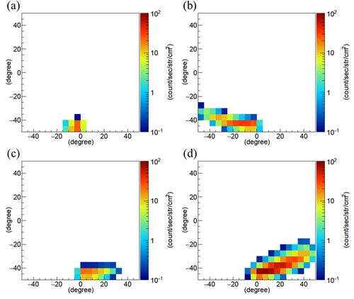
The inverse analysis domain was the same as the real-time high-resolution atmospheric dispersion simulation domain. In this domain, four ETCCs were located at the four corners (NE, SE, SW, NW) of the analysis domain as shown in Figure 6, which are about 283 m away from the release point, i.e. the center of the domain, to cover the whole domain within the field of view (100 degrees) of each ETCC. The view angle of each ETCC was set in the direction of the release point with a 50-degree elevation angle. The gamma-ray images for the 662-keV gamma-ray of ¹³⁷Cs were then generated by applying the gamma-ray response function matrices prepared for these ETCCs to the 3D distribution of ¹³⁷Cs by the calculation of the ground truth. Figure 7 shows the hypothetical gamma-ray images by ETCCs for the 622-keV gamma-ray of ¹³⁷Cs for the first 1-min period. In these gamma-ray images, a unit value of gamma-ray intensity (1.0 count str⁻¹ sec⁻¹ cm⁻²) is converted into 137 count min⁻¹ at each angular area of ETCC (5 × 5 degrees), applying the effective detection area (300 cm²) of the ETCC. However, the detection rate of gamma-ray at each angular area decreased to 0.02 count min⁻¹, considering the detection efficiency (1.5 × 10⁻⁴) by TPC of the current ETCC for the 662-keV gamma-ray. This indicates that the angular area with values over 50 count str⁻¹ sec⁻¹ cm⁻² in Figure 7 of the current ETCC has a possibility to capture more than one incident events of 662-keV gamma-ray of ¹³⁷Cs from the plume during the 1-min period in this analysis configuration. Therefore, the longer time interval (e.g. 10 min) to accumulate gamma-ray is necessary to obtain the gamma-ray image for this test case, while the case with the 10 times release rate, which is comparable to the release rate of ¹³⁷Cs at the time of the hydrogen explosion at unit 1 of FDNPS, is high enough to generate the gamma-ray image in a 1-min interval. Since the current ETCC was designed to enhance the mobility for utilization in the reactor buildings of FDNPS, it has detection limitation for application in the present test cases. However, for this kind of monitoring purpose, the detection limit of ETCC can be improved by more than an order of magnitude using a larger size of TPC and different types of gas with a larger cross section of Compton scattering in TPC (e.g. CF₄ has a 2.3 times larger cross section of Compton scattering than Ar gas currently used) [29].

Figure 6. Inverse analysis domain setting. Green marks and arrows at the four corners of the domain indicated the locations and horizontal view angles of ETCCs. Examples of gamma-ray images at ETCC locations are also shown.

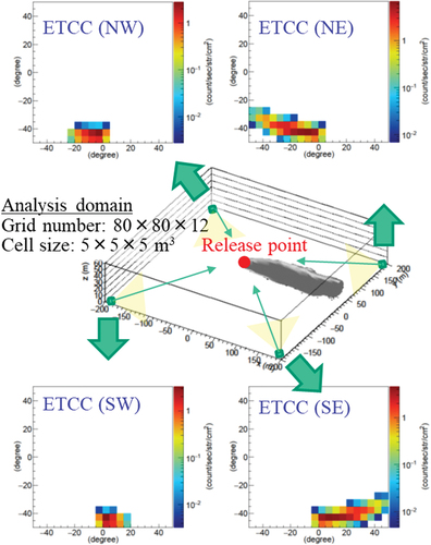
Figure 7. Hypothetical gamma-ray images by ETCCs located at (a) NW, (b) NE, (c) SW, and (d) SE corners of the analysis domain for the 622-keV gamma-ray of ¹³⁷Cs for the first 1-min period of the test case.

3. Results and discussion

3.1. Optimization of the tunable parameters

The tunable parameters, iteration number I and scaling factor A, in the inverse analysis method were determined by sensitivity analysis using the test data for the first release period. The sensitivity analysis was performed for the 40 cases by changing the parameter values as I = 80, 100, 120, and 140 and A = 0.1, 0.2, 0.5, 1, 2, 5, 10, 20, 50, and 100 around likely values of I = 100 or 120 and A = 1–10 found by trial and error. The optimum values for I and A were determined to mostly reproduce the air concentration pattern of the ground truth. The fraction of air concentrations of analysis results within a factor of two (FAC2) in comparison to those of ground truth that exceed a certain significant concentration value (1.0 × 10⁵ Bq m⁻³ in this case) was used to evaluate the reproducibility of air concentration. FAC2 is widely used to evaluate the performance of local-scale atmospheric dispersion models. For instance, Hanna and Chang [54] suggested FAC2 ≥ 50% and FAC2 ≥ 30% as the acceptance criteria for rural and urban dispersion simulations, respectively.

Table 1 summarizes the release rate and the maximum air concentration for the ground truth, the prior condition, and the inverse analysis results for 40 cases and FAC2 in comparison of the ground truth with the prior condition and 40 cases. Regarding the prior condition, air concentrations were normalized by applying the release rate of the ground truth (1.0 × 10¹⁰ Bq s⁻¹). Using a single CPU of PC (Intel Core i7-6700K, 4.00 GHz), the computational times of the inverse analysis for these cases were about 27 s with only a 1-s increase by using larger I. This difference was not considered in the selection of the optimum values. The optimum values for I and A were selected as I = 100 and A = 10, considering the reproducibility of air concentration pattern based on FAC2 (55.43%) and the maximum concentration (7.329 × 10⁷ Bq m⁻³, about 0.5% higher than the ground truth value, 7.290 × 10⁷ Bq m⁻³). In this case, the estimated release rate was 1.033 × 10¹⁰ Bq m⁻³, which is 3% higher value than the actual release rate. The comparison of the distribution patterns of air concentrations of the ground truth with this case and the prior condition normalized by applying the release rate are shown as scatterplots and contour maps in Figures 8 and 9, respectively. These results demonstrated how the distribution pattern of the prior condition was corrected by the inverse analysis from the gamma-ray images. However, in this ideal and simple condition, the prior condition might happen to be favorable to this analysis, although it was generated using a different model and wind field from the ground truth. Therefore, the analysis method needs to be examined using more realistic and complex conditions in the future study.

Figure 8. Scatterplots of air concentrations of ¹³⁷Cs comparing the ground truth with (a) the prior condition normalized by applying the release rate and (b) inverse analysis result of the optimum case for the first 1-min period of the test case. The solid and broken lines indicate the perfect and FAC2 lines, respectively.

Figure 9. Horizontal distributions of air concentrations of ¹³⁷Cs at the level of the release height for (a) the ground truth, (b) inverse analysis result of the optimum case, and (c) the prior condition normalized by applying the release rate for the first 1-min period of the test case.

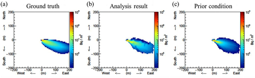
Table 1. Release rate and the maximum air concentration for the ground truth, the prior condition, and the inverse analysis results for 40 cases for the first 1-min period and FAC2 comparing air concentrations between the ground truth and analysis results.

Analysis case	Release rate (10^10 Bq s^−1)	Maximum concentration (10^7 Bq m^−3)	FAC2 (%)
The ground truth	1.000	7.290	-
The prior condition (normalized by applying the release rate)	1.000	8.246	27.74
I = 80, A = 0.1	1.113	9.729	39.93
I = 80, A = 0.2	1.087	9.603	43.37
I = 80, A = 0.5	1.060	9.165	48.66
I = 80, A = 1	1.043	8.535	51.68
I = 80, A = 2	1.031	7.714	53.49
I = 80, A = 5	1.028	7.237	54.16
I = 80, A = 10	1.029	7.225	54.13
I = 80, A = 20	1.033	7.661	53.95
I = 80, A = 50	1.039	7.645	51.27
I = 80, A = 100	1.045	7.957	47.92
I = 100, A = 0.1	1.104	9.717	42.33
I = 100, A = 0.2	1.075	9.575	46.54
I = 100, A = 0.5	1.048	9.090	52.60
I = 100, A = 1	1.039	8.422	55.17
I = 100, A = 2	1.033	7.539	55.28
I = 100, A = 5	1.033	7.199	55.05
I = 100, A = 10	1.033	7.329	55.43
I = 100, A = 20	1.032	7.524	54.10
I = 100, A = 50	1.039	7.566	52.15
I = 100, A = 100	1.049	8.026	48.94
I = 120, A = 0.1 I = 120, A = 0.2	1.096 1.064	9.706 9.547	43.84 49.58
I = 120, A = 0.5	1.039	9.022	54.50
I = 120, A = 1	1.032	8.315	55.79
I = 120, A = 2	1.030	7.384	54.66
I = 120, A = 5	1.032	7.146	54.06
I = 120, A = 10	1.030	7.247	54.35
I = 120, A = 20	1.029	7.328	52.46
I = 120, A = 50	1.038	7.411	50.58
I = 120, A = 100	1.051	7.926	47.38
I = 140, A = 0.1	1.089	9.696	45.22
I = 140, A = 0.2	1.057	9.520	51.72
I = 140, A = 0.5	1.034	8.960	54.91
I = 140, A = 1	1.030	8.221	55.24
I = 140, A = 2	1.030	7.260	52.79
I = 140, A = 5	1.032	7.110	52.38
I = 140, A = 10	1.030	7.125	51.80
I = 140, A = 20	1.031	7.183	49.95
I = 140, A = 50	1.042	7.345	46.92
I = 140, A = 100	1.057	7.876	44.51

3.2. Reproducibility for the temporal changes in release rate

The reproducibility of the inverse analysis method optimized in the previous section was examined for the second 1-min period using the cases with temporal change in release rate. For these cases, the computational times of the inverse analysis were about 27 s, which did not increase from the analysis for the first 1-min period. It is because the inverse matrix calculation in Equation (11)(11) $J=[{\left(\mathit{R}\mathit{x}-\mathit{y}\right)}^{T}C{\left(\mathit{y}\right)}^{-1}\left(\mathit{R}\mathit{x}-\mathit{y}\right)\text{break}+{\left(\mathit{x}-r{\mathit{x}}_0\right)}^{T}C{\left(r{\mathit{x}}_0\right)}^{-1}\left(\mathit{x}-r{\mathit{x}}_0\right)]/2,$(11) occupied most of the computational times, and the matrix sizes were almost the same for these cases. This means that the computational time in this analysis configuration is short enough to apply for the real-time utilization. Therefore, this analysis can be coupled with WSPEEDI-DB [14] to immediately reveal the spatiotemporal distribution of the released radioactive materials in larger scales for emergency countermeasures.

Table 2 summarizes the release rate and the maximum air concentration for the second 1-min period by the ground truth and the inverse analysis results for the five cases. It was shown that the release rates for the second 1-min period were 0.1, 0.5, 1.0, 2.0, and 10.0 times the release rate for the first 1-min period. Moreover, FAC2 compared air concentrations between the ground truth and analysis results. The estimated release rates by the inverse analysis were about 5.39, 1.89, 1.47, 1.25, and 1.06 times larger than those of the ground truth for the cases with 0.1, 0.5, 1.0, 2.0, and 10.0 times the release rate, respectively. Having the same or larger release rates resulted in the reproduction of release rates with rather smaller overestimation. On the other hand, when the release rates became smaller, the reproduced release rates were significantly overestimated. This is because the smaller the release rates for the second period became, the more significantly they were affected by errors in the process to make adjusted gamma-ray images for the second estimation period by subtracting the contribution from radioactivity released in the first period. One of the factors causing the errors was the treatment to remove negative values in the adjusted gamma-ray images by substituting 0. Although this needs to be improved, the overestimation of the release rate when it becomes smaller can be accepted as a conservative estimation.

Table 2. Release rate and the maximum air concentration for the second 1-min period by the ground truth and the inverse analysis results for the five cases, in which the release rates for the second 1-min period were 0.1, 0.5, 1.0, 2.0, and 10.0 times the release rate of the first 1-min period, together with FAC2 comparing air concentrations between the ground truth and analysis results.

Release rate change (times)	Release rate (10^10 Bq s^−1)		Maximum concentration (10^7 Bq m^−3)		FAC2 (%)
	The ground truth	Inverse analysis	The ground truth	Inverse analysis
0.1	0.100	0.539	0.862	1.872	2.83
0.5	0.500	0.945	4.353	4.662	23.99
1.0	1.000	1.469	8.459	9.678	28.88
2.0	2.000	2.499	17.980	21.124	30.25
10.0	10.000	10.606	85.216	103.713	28.04

For the maximum concentrations, the estimated values were about 2.17, 1.07, 1.14, 1.17, and 1.22 times larger than those of the ground truth for the cases with 0.1, 0.5, 1.0, 2.0, and 10.0 times the release rate, respectively. The FAC2 values were about 24%–30%, which were not satisfied but close to the acceptance criteria (30%) for the cases except for the significant low values of 2.83 for the case with 0.1 time the release rate. As scatterplots, Figure 10 shows the comparison of the distribution patterns of air concentrations of the ground truth with these cases. The air concentrations by the inverse analysis tended to overestimate the ground truth for the range with lower concentration, and this tendency caused the low FAC2 values. This indicated that the gamma-ray contribution from radioactivity released in the previous period was not subtracted completely. However, considering the many factors of errors, such as release rate change and dispersion calculation for the previous release period, among others, the air concentration patterns for the second 1-min period were reasonably reproduced by the inverse analysis.

Figure 10. Scatterplots of air concentrations of ¹³⁷Cs comparing the ground truth with the inverse analysis results for the cases with (a) 0.1, (b) 0.5, (c) 1.0, (d) 2.0, and (e) 10.0 times the release rate. The solid and broken lines indicate the perfect and FAC2 lines, respectively.

3.3. Influence of the limited analysis domain

In this inverse analysis, the hypothetical gamma-ray images by ETCC were generated using only the air concentration data within the analysis domain (400 m × 400 m in the horizontal direction). However, air concentrations outside the analysis domain also contribute to gamma-ray images in the actual condition. This influence on the inverse analysis was evaluated by applying modified gamma-ray images that were generated using the air concentration data of LOHDIM-LES within the extended domain (800 m × 800 m in the horizontal direction). The inverse analysis results using the modified gamma-ray images were almost the same as the original analysis results for the first 1-min period, since the air concentration by LOHDIM-LES was distributed mostly within the inverse analysis domain. Therefore, the influence was evaluated with the results for the second 1-min period, when a significant portion of the radioactivity released in the first 1-min period had flowed out the analysis domain.

Table 3 summarizes the release rate and the maximum air concentration for the second 1-min period by the original and modified inverse analysis results for the five cases with the release rate changes together with FAC2 comparing air concentrations between the original and modified analysis results. The estimated release rates and maximum air concentrations by the modified analysis were almost the same as those by the original analysis except for the case with 0.1 time the release rate (about 15% and 30% increase for release rate and maximum air concentration, respectively). FAC2 values were very high, i.e. 88.2% for the case with 0.1 time the release rate and more than 90% for the other cases. These results suggest that the influence of the limited analysis domain that excluded the gamma-ray contribution from the radioactivity outside the domain on the inverse analysis was small. It can be explained by the fact that the view area of the ETCC located at the side of the domain where the plume flowed out almost overlapped with the analysis domain and did not capture the gamma-ray from outside of the domain, while the ETCC located at the opposite side of the domain captured only sufficiently attenuated gamma-ray from the remote plume outside of the domain. Considering the increase in computational times for both the inverse analysis and the real-time high-resolution atmospheric dispersion simulation using a larger domain, this analysis configuration with the limited domain was reasonable to achieve a balance between the accuracy in analysis results and the processing speed for the real-time utilization.

Table 3. Release rate and the maximum air concentration for the second 1-min period by the original and modified inverse analysis results for the five cases, in which the release rates for the second 1-min period were 0.1, 0.5, 1.0, 2.0, and 10.0 times the release rate of the first 1-min period, together with FAC2 comparing air concentrations between the original and modified analysis results.

Release rate change (times)	Release rate (10^10 Bq s^−1)		Maximum concentration (10^7 Bq m^−3)		FAC2 (%)
	Original analysis	Modified analysis	Original analysis	Modified analysis
0.1	0.539	0.620	1.872	2.427	88.18
0.5	0.945	0.984	4.662	4.762	91.34
1.0	1.469	1.505	9.678	8.966	94.38
2.0	2.499	2.536	21.124	21.047	96.29
10.0	10.606	10.636	103.713	103.834	99.63

3.4. Applicability to other radionuclides and possibility of the validation using actual data

This section investigates the applicability of the inverse analysis method to radionuclides other than ¹³⁷Cs tested above and discusses the possibility of the validation using an actual atmospheric release of radionuclide. The other radionuclides investigated in this study include ¹³⁴Cs, ¹³¹I, ¹³²I, ¹³³I, ¹³²Te, and ¹³³Xe, which were used for the dose assessment of the FDNPS accident by UNSCEAR [13]. Table 4 summarizes the characteristics of these radionuclides, gamma-ray energies, emission rates, and attenuation coefficients in air. It also contains the maximum values of the hypothetical direct gamma-ray intensities by the ETCC generated using the same air concentration distribution for the first 1-min period. Although the hypothetical gamma-ray intensities by the ETCC for radionuclides, except for ¹³⁴Cs, were lower than that for ¹³⁷Cs, these values would become much higher than that for ¹³⁷Cs in the actual release condition in a nuclear accident because the estimated release rates of these radionuclides due to the FDNPS accident had 1–2-order higher values than ¹³⁷Cs. For example, 10 times higher values for ¹³¹I, ¹³²I, ¹³³I, and ¹³²Te and 40 times higher values for ¹³³Xe during the hydrogen explosion at unit 1 of FDNPS were used for the dose assessment in the UNSCEAR 2013 report [55]. The proposed analysis method is applicable to other major radionuclides similarly to ¹³⁷Cs. However, gamma-ray energy peaks of some radionuclides (e.g. 662 keV of ¹³⁷Cs and 668 keV of ¹³²I) are overlapped in the energy resolution of ETCC and cannot be simply distinguished from each other in the condition of multiple radionuclides release. Therefore, a combined analysis for multiple radionuclides needs to be examined in the next step to obtain the temporal change in composition of these radionuclides, which was not correctly determined in the source term of the FDNPS accident.

Table 4. Characteristics of radionuclides, gamma-ray energies, emission rates, and attenuation coefficients in air for ¹³⁷Cs, ¹³⁴Cs, ¹³¹I, ¹³²I, ¹³³I, ¹³²Te, ¹³³Xe, and ⁸⁵Kr, and the maximum values of the hypothetical gamma-ray intensities by ETCC for these radionuclides generated using the same air concentration distribution for the first 1-min period.

Radionuclide	Gamma-ray energy (keV)	Emission rate (%)	Attenuation coefficient (cm^2 g^−1)	Maximum gamma-ray (count str^−1 sec^−1 cm^−2)
^137Cs	662	85.1	7.701 × 10^−2	98.8
^134Cs	605	97.6	8.025 × 10^−2	104.1
^131I	364	81.7	9.906 × 10^−2	53.2
^132I	955	17.6	6.500 × 10^−2	28.1
^133I	530	87.0	8.496 × 10^−2	82.0
^132Te	228	88.0	11.777 × 10^−2	35.2
^133Xe	81	38.0	16.550 × 10^−2	4.4
^85Kr	514	0.43	8.590 × 10^−2	0.4

The possibility of the validation of the analysis method was also investigated using the actual release of ⁸⁵Kr from a nuclear fuel reprocessing plant. When spent fuels are reprocessed, radionuclides, such as ⁸⁵Kr, ³H, ¹⁴C, and ¹²⁹I, are discharged into the atmosphere under a release control. The air concentrations of these radionuclides and the air dose rates were measured during the test operations of reprocessing using actual spent fuels at the nuclear reprocessing plant in Rokkasho (RRP), Japan, from March 2006 to October 2008. These data were successfully utilized in the model validation for the atmospheric dispersion and air dose rate calculation [41]. In this case, the air dose rate measured at monitoring posts was mainly caused by the gamma-ray from ⁸⁵Kr. Table 4 also summarizes the gamma-ray energies, emission rates, and attenuation coefficients in air for ⁸⁵Kr and the maximum value of hypothetical direct gamma-ray intensity by ETCC. The release rate (1.0 × 10¹⁰ Bq s⁻¹) used in this test is comparable to the release rate of ⁸⁵Kr during the test operations at RRP [56]. The estimated maximum gamma-ray intensity (0.4 count str⁻¹ sec⁻¹ cm⁻²) is too low compared to the lowest intensity level (about 50 count str⁻¹ sec⁻¹ cm⁻²) for each angular area of the current ETCC to capture an incident event of the gamma-ray for a 1-min interval in this test configuration. This is also the same for the modified ETCC for monitoring purpose with more than 10 times higher sensitivity than the current one. However, if the modified ETCCs were set closer to the release point, lower angular resolution of gamma-ray image was used, for example, half the distance and angular area with 10 × 10 degrees, respectively, and gamma-ray was continuously accumulated for 1 h, the gamma-ray intensity increases up to 9600 (10 × 4 × 4 × 60) times higher value. Therefore, there is a possibility for the ETCC to capture direct gamma-ray images due to the actual release of ⁸⁵Kr from RRP during its operation.

4. Conclusion

This study demonstrated the feasibility of the inverse analysis in a novel monitoring method for the quantitative visualization of 3D distribution of a radioactive plume and source term of released radionuclides by combining gamma-ray imaging spectroscopy with the ETCC and real-time high-resolution atmospheric dispersion simulation based on 3D wind observation with Doppler lidar. In this method, 3D distribution of each radionuclide in the radioactive plume is inversely reconstructed from direct gamma-ray images of each radionuclide by several ETCCs located around the target by harmonizing with the air concentration distribution pattern of the plume predicted by real-time atmospheric dispersion simulation.

A prototype of this analysis method was tested with cases using hypothetical data generated by numerical simulations of atmospheric dispersion and radiation transport. The performance of the first and the second steps of analysis procedure (Figure 5) was investigated to obtain the temporal changes with a 1-min interval in release rate and 3D distribution of radioactive plume. For both steps, the computational times of the inverse analysis were about 27 s using a single CPU of PC (Intel Core i7-6700K, 4.00 GHz), which is short enough to apply for the real-time utilization. For the first 1-min period, the value of the release rate and the maximum concentration was estimated as 3% higher than the ground truth, and the air concentration pattern was well reproduced with a high FAC2 value (55.43%). For the second 1-min period, the release rate changes with 0.1, 0.5, 1.0, 2.0, and 10.0 times from the first period were tested. While the release rates were reproduced with rather smaller overestimation when the release rates were the same or became larger, they were significantly overestimated when the release rates became smaller. The concentration patterns were reproduced with acceptable FAC2 values (24%–30%) except for the case with 0.1 times the release rate. This indicated that the gamma-ray contribution from the radioactivity released in the previous period was not subtracted completely. Although this needs to be improved, the overestimation when the release rate becomes smaller can be accepted as a conservative estimation. It was also shown that the influence of the limited analysis domain (400 m × 400 m in the horizontal direction) on the inverse analysis was small, and this analysis configuration was reasonable to achieve a balance between the accuracy in analysis results and the processing speed for the real-time utilization. Furthermore, it was shown that the proposed method is applicable to other major radionuclides, such as ¹³⁴Cs, ¹³¹I, ¹³²I, ¹³³I, ¹³²Te, and ¹³³Xe, for the dose assessment in case of a nuclear accident and has a possibility to be validated using the actual release of ⁸⁵Kr from a nuclear fuel reprocessing plant. Once the feasibility of the analysis method was shown in this ideal and simple condition, more realistic and complex conditions, such as the release of multiple radionuclides, influence of errors in gamma-ray images and dispersion calculations, and various atmospheric stability conditions, are planned to be examined in the future study.

Both ETCC and Doppler lidar can measure the target objects remotely and constantly. Therefore, the proposed method with these monitors can detect the outbreak of discharge of radioactive materials by installing at any place in the target nuclear facility and monitoring from the beginning of nuclear accident. This method is expected to become an innovative monitoring framework for nuclear emergency with flexibility and robustness against disasters. Furthermore, using the source term estimated by this analysis, WSPEEDI-DB [14] and its real-time application method [17] can immediately output calculation results of spatiotemporal distribution of the released radioactive materials in larger scales. While these results are the present state analysis around the nuclear facility, they can provide the future prediction of the radioactive plume behavior in areas with some distance away from the release point. Besides these prediction results, the information on uncertainty in forecasted plume directions generated by the additional function of WSPEEDI-DB [15,16] are useful for emergency countermeasures.

Acknowledgments

The authors express their gratitude to Prof. Toru Tanimori of Kyoto University for providing the information about ETCC and his helpful comments and suggestions.

Disclosure statement

No potential conflict of interest was reported by the authors.

Additional information

Funding

This work was supported by the JAEA Nuclear Energy S&T and Human Resource Development Project Grant Number JPJA18P18071754 and JPJA22P22682536.

References

- Imai K, Chino M, Ishikawa H. SPEEDI: a computer code system for the real-time prediction of radiation dose to the public due to an accidental release. JAERI–1297. Japan: Japan Atomic Energy Research Institute; 1985. p. 93.
- Ministry of Education, Culture, Sports Science and Technology (MEXT). Review of response by MEXT concerning the recovery from the Great East Japan Earthquake, July 27. 2012 (Available from https://www.mext.go.jp/a_menu/saigaijohou/syousai/1323699.htm, last access: November 2022) [in Japanese].
- Terada H, Chino M. Development of an atmospheric dispersion model for accidental discharge of radionuclides with the function of simultaneous prediction for multiple domains and its evaluation by application to the chernobyl nuclear accident. J Nucl Sci Technol. 2008;45(9):920–931.
- Chino M, Nakayama H, Nagai H et al. Preliminary estimation of release amounts of 131I and 137 Cs accidentally discharged from the fukushima daiichi nuclear power plant into the atmosphere. J Nucl Sci Technol. 2011;48(7):1129–1134.
- Katata G, Nagai H, Terada H et al. Numerical reconstruction of high dose rate zones due to the Fukushima Dai-ichi Nuclear Power Plant accident. J Environ Radioact. 2012;111:2–12.
- Katata G, Ota M, Terada H et al. Atmospheric discharge and dispersion of radionuclides during the Fukushima Dai-ichi Nu-clear Power Plant accident. Part I: source term estimation and local-scale atmospheric dispersion in early phase of the accident. J Environ Radioact. 2012;109:103–113.
- Terada H, Katata G, Chino M et al. Atmospheric discharge and dispersion of radionuclides during the Fukushima Daiichi Nu-clear Power Plant accident. Part II: verification of the source term and regional-scale atmospheric dispersion. J Environ Radioact. 2012;112:141–154.
- Kobayashi T, Nagai H, Chino M et al. Source term estimation of atmospheric release due to the Fukushima Dai-ichi Nuclear Power Plant accident by atmospheric and oceanic dispersion simulations. J Nucl Sci Technol. 2013;50(3):255–264.
- Katata G, Chino M, Kobayashi T et al. Detailed source term estimation of the atmospheric release for the Fukushima Daiichi Nuclear Power Station accident by coupling simulations of an atmospheric dispersion model with an improved deposition scheme and oceanic dispersion model. Atmos Chem Phys. 2015;15(2):1029–1070.
- Chino M, Terada H, Nagai H et al. Utilization of 134Cs/137Cs in the environment to identify the reactor units that caused atmospheric releases during the Fukushima Daiichi accident. Sci Rep. 2016;6(1):31376.
- Terada H, Nagai H, Tsuduki K et al. Refinement of source term and atmospheric dispersion simulations of radionuclides during the Fukushima Daiichi Nuclear Power Station accident. J Environ Radioact. 2020;213:106104.
- Ohba T, Ishikawa T, Nagai H et al. Reconstruction of residents’ thyroid equivalent doses from internal radionuclides after the Fukushima Daiichi nuclear power station accident. Sci Rep. 2020;10(1). DOI:10.1038/s41598-020-60453-0
- UNSCEAR (United Nations Scientific Committee on the Effects of Atomic Radiation). UNSCEAR 2020/2021 Report: sources, Effects and Risks of Ionizing Radiation. New York: United Nations; 2022Vol. Vol. IIp 241.
- Terada H, Nagai H, Tanaka A et al. Atmospheric-dispersion database system that can immediately provide calculation results for various source term and meteorological conditions. J Nucl Sci Technol. 2020;57(6):745–754.
- Yoshida T, Nagai H, Terada H et al. Evaluation of uncertainties derived from meteorological forecast inputs in plume directions predicted by atmospheric dispersion simulations. J Nucl Sci Technol. 2022;59(1):55–66.
- Kadowaki M, Nagai H, Yoshida T et al. Application of Bayesian machine learning for uncertainty estimation of plume directions using atmospheric dispersion simulations. J Nucl Sci Technol. 2023;1–14. DOI:10.1080/00223131.2023.2177763
- Terada H, Nagai H, Kadowaki M et al. Dependency of the source term estimation method for radionuclides released into the atmosphere on the available environmental monitoring data and its applicability to real-time source term estimation. J Nucl Sci Technol. 2023;1–22. DOI:10.1080/00223131.2022.2162139
- Nuclear Regulation Authority (NRA). Emergency monitoring: a supplementary reference material of the nuclear emergency response guidelines ( revised in 2021). 2014 (Available from https://www.nra.go.jp/data/000276389.pdf, last access: November 2022) [in Japanese].
- Hirayama H, Matsumura H, Namito Y et al. Estimation of Xe-135, I-131, I-132, I-133 and Te-132 Concentrations in Plumes at Monitoring Posts in Fukushima Prefecture Using Pulse Height Distribution Obtained from NaI(Tl) Detector. Trans at Energy Soc Jpn. 2017;16(1):1–14. in Japanese. 10.3327/taesj.J16.014.
- Terasaka Y, Yamazawa H, Hirouchi J et al. Air concentration estimation of radionuclides discharged from Fukushima Daiichi Nuclear Power Station using NaI(Tl) detector pulse height distribution measured in Ibaraki Prefecture. J Nucl Sci Technol. 2016;53(12):1919–1932.
- Moriizumi J, Oku A, Yaguchi N et al. Spatial distributions of atmospheric concentrations of radionuclides on 15 March 2011 discharged by the Fukushima Dai-Ichi Nuclear Power Plant Accident estimated from NaI(Tl) pulse height distributions measured in Ibaraki Prefecture. J Nucl Sci Technol. 2020;57(5):495–513.
- Takeda S, Harayama A, Ichinohe Y et al. A portable Si/CdTe Compton camera and its applications to the visualization of radioactive substances. Nucl Instr Meth Phys Res A. 2015;787:207–211.
- Jiang J, Shimazoe K, Nakamura Y et al. A prototype of aerial radiation monitoring system using an unmanned helicopter mounting a GAGG scintillator Compton camera. J Nucl Sci Technol. 2016;53(7):1067–1075.
- Vetter K. Multi-sensor radiation detection, imaging, and fusion. Nucl Instr Meth Phys Res A. 2015;805:127–134.
- Kagaya M, Katagiri H, Enomoto R et al. Development of a low-cost-high-sensitivity Compton camera using CsI (Tl) scintillators (γ I). Nucl Instr Meth Phys Res A. 2015;804:25–32.
- Sato Y, Terasaka Y. Radiation imaging using an integrated radiation imaging system based on a compact Compton camera under unit 1/2 exhaust stack of Fukushima Daiichi Nuclear Power Station. J Nucl Sci Technol. 2022;59(6):677–687.
- Okada K, Tadokoro T, Ueno Y et al. Development of a gamma camera to image radiation fields. Prog Nucl Sci Tech. 2014;4:14–17.
- Tanimori T, Kubo H, Takada A et al. An electron-tracking Compton telescope for a survey of the deep universe by MeV gamma rays. Astrophys J. 2015;810(1):28.
- Tanimori T, Mizumura Y, Takada A et al. Establishment of Imaging Spectroscopy of Nuclear Gamma-Rays based on Geometrical Optics. Sci Rep. 2017;7(1):41511.
- Takada A, Kubo H, Nishimura H et al. Observation of Diffuse Cosmic and Atmospheric Gamma Rays at Balloon Altitudes with an Electron-Tracking Compton Camera. Astrophys J. 2011;733(1):13.
- Kabuki S, Kimura H, Amano H et al. Electron-Tracking Compton Gamma-Ray Camera for small animal and phantom imaging. Nucl Instr Meth Phys Res A. 2010;623(1):606–607.
- Mizumoto T, Tomono D, Takada A et al. A performance study of an electron-tracking Compton camera with a compact system for environmental gamma-ray observation. J Instrum. 2015;10(06):C01053.
- Tomono D, Mizumoto T, Takada A et al. First On-Site True Gamma-Ray Imaging-Spectroscopy of Contamination near Fukushima Plant. Sci Rep. 2017;7(1):41972.
- Nakayama H, Yoshida T, Terada H et al. Toward Development of a Framework for Prediction System of Local-Scale Atmospheric Dispersion Based on a Coupling of LES-Database and On-Site Meteorological Observation. Atmosphere. 2021;12(7):899.
- Collaborative Laboratories for Advanced Decommissioning Science, Fukushima Research Institute, Sector of Fukushima Research and Development and Kyoto University Quantitative Analysis of Radioactivity Distribution by Imaging of High Radiation Field Environment using Gamma-ray Imaging Spectroscopy (Contract Research)-FY2020 Nuclear Energy Science & Technology and Human Resource Development Project-JAEA-Review 2022-027, 85pp, 2022, DOI:10.11484/jaea-review-2022-027 [in Japanese].
- Nakayama H, Nagai H. Development of local-scale high-resolution atmospheric dispersion model using Large-Eddy simulation Part 1: turbulent flow and plume dispersion over a flat terrain. J Nucl Sci Technol. 2009;46(12):1170–1177.
- Nakayama H, Nagai H. Development of local-scale high-resolution atmospheric dispersion model using large-eddy simulation Part 2: turbulent flow and plume dispersion around a cubical building. J Nucl Sci Technol. 2011;48(3):374–383.
- Nakayama H, Jurcakova K, Nagai H. Development of local-scale high-resolution atmospheric dispersion model using large-eddy simulation Part 3: turbulent flow and plume dispersion in building arrays. J Nucl Sci Technol. 2013;50(5):503–519.
- Nakayama H, Leitl B, Harms F, et al. Development of local-scale high-resolution atmospheric dispersion model using large-eddy simulation Part 4: turbulent flows and plume dispersion in an actual urban area. J Nucl Sci Technol. 2014;51(5):626–638. DOI:10.1080/00223131.2014.885400
- Nakayama H, Takemi T, Nagai H. Development of Local-scale High-resolution atmospheric Dispersion Model using Large-Eddy Simulation. Part 5: detailed simulation of turbulent flows and plume dispersion in an actual urban area under real meteorological conditions. J Nucl Sci Technol. 2016;53(6):887–908.
- Nakayama H, Satoh D, Nagai H et al. Development of local-scale high-resolution atmospheric dispersion model using large-eddy simulation Part 6: introduction of detailed dose calculation method. J Nucl Sci Technol. 2021;58(9):949–969.
- Nakayama H, Onodera N, Satoh D et al. Development of local-scale high-resolution atmospheric dispersion and dose assessment system. J Nucl Sci Technol. 2022;59(10):1314–1329.
- Smagorinsky J. General circulation experiments with the primitive equations. Mon Weather Rev. 1963;91(3):99–164.
- Goldstein D, Handler R, Sirovich L. Modeling a no-slip flow boundary with an external force field. J. Comput. Phys. 1993;105(2):354–366.
- Cheng H, Castro IP. Near wall flow over urban-like roughness. Bound. Layer Meteorol. 2002;104(2):229–259.
- IEC61400-1.Wind Turbines Part 1: design Requirements. 3rd ed. Geneva, Switzerland: International Electrotechnical Commission; 2005.
- Yamada T, Bunker S. Development of a nested grid, second moment turbulence closure model and application to the 1982 ASCOT Brush Creek data simulation. J Appl Meteorol Climatol. 1988;27(5):562–578.
- Gurney KR, Law RM, Denning AS et al. TransCom 3 CO2 inversion intercomparison: 1. Annual mean control results and sensitivity to transport and prior flux information. Tellus. 2003;55(2):555–579.
- Enting IG. Inverse Problems in Atmospheric Constituent Transport. 392pp. Cambridge: Cambridge University PressU. K; 2002.
- Tarantola A. Inverse Problem Theory. 600pp. Amsterdam: Elsevier; 1987.
- Nakayama H, Takemi T. Large-eddy simulation studies for predicting plume concentrations around nuclear facilities using an overlapping technique. Int J Environ Pollut. 2018;64(1/2/3):125–144.
- Kataoka H, Mizuno M. Numerical flow computation around aeroelastic 3D square cylinder using inflow turbulence. Wind Struct. 2002;5(2_3_4):379–392.
- Monin A, Obukhov M. Basic laws of turbulent mixing in the ground layer of the atmosphere. Tr. Akad. Nauk SSSR Geophiz. Inst. 1954;24:163–187.
- Hanna SR, Chang JC. Acceptance criteria for urban dispersion model evaluation. Meteorol Atmos Phys. 2012;116(3–4):133–146.
- UNSCEAR (United Nations Scientific Committee on the Effects of Atomic Radiation). UNSCEAR 2013 Report: sources, Effects and Risks of Ionizing Radiation. New York: United Nations; 2014Vol. Vol. Ip 311.
- Terada H, Nagai H, Yamazawa H. Validation of a Lagrangian atmospheric dispersion model against middle-range scale measurements of 85Kr concentration in Japan. J Nucl Sci Technol. 2013;50(12):1198–1212.