Uncertainty quantification of unconfined spill fire data by coupling Monte Carlo and artificial neural networks

ABSTRACT

Due to the complexity of spill fire, predicting heat release rate (HRR) is a challenging aspect, therefore, identifying key contributors to uncertainty is essential to develop reliable models for fire risk assessment. We propose a framework that couples Artificial-Neural-Network (ANN) and Monte Carlo Uncertainty Quantification (UQ) to quantify the uncertainties of spill fire parameters on peak HRR variance. The ANN spill fire model, trained on experimental spill fire data, shows good agreement with measured HRR values. By coupling with Dakota for Monte Carlo uncertainty propagation, the framework identifies major contributors to peak HRR uncertainty for fixed and continuous unconfined spill fires. This is achieved by investigating two uncertainty sources: data scarcity and input parameters. UQ results indicate that the confidence intervals widen at points where data are scarcer. Sensitivity analysis shows that in the case of fixed quantity spills, the fuel amount and properties parameters contribute to 54.4% and 22.6% of peak HRR variance, respectively. For continuous spills, the discharge rate and fuel properties parameters account for 41.8% and 39.3% of peak HRR variance, respectively. This work can be utilized in developing more advanced predictive ANN models for spill fire scenarios, ultimately enhancing fire probabilistic safety analysis in nuclear power plants.

KEYWORDS:

• Spill fire
• uncertainty quantification
• sensitivity analysis
• artificial neural network
• Dakota
• Monte Carlo

1. Introduction

Uncertainty Quantification (UQ) methodologies aim to assess and manage uncertainties associated with experimental data and numerical models, allowing for more reliable predictions and improved decision-making process. The evaluation of input parameters’ uncertainty is a critical aspect of UQ as it can significantly influence the model outputs and subsequent risk assessments. Spill fires are a risk-significant scenario representing 9.2% of the challenging historical fire events in nuclear power plants (NPPs) in the U.S. from 1990 to 2014 [1]. Spill fires are inherently complex and dynamic, introducing a multitude of uncertainties that further compound the challenges of an accurate consequence analysis [2]. This work aims to improve spill-fire UQ by proposing a coupling of machine learning with Dakota computational tool to identify sources of uncertainties in the peak HRR based on a multivariate experimental database.

In the realm of fire risk assessment, earlier studies have examined the process of addressing uncertainties connected with fire data. Siu et al. [3,4] examined uncertainties in fire risk assessment for large-compartment fires in NPPs using analytical models to propagate parameter uncertainties. Ho et al. [5,6] developed the COMPBRN computational model, which focused on uncertainties in the burning rate, air entrainment, plume, and wall heat transfer processes using expert judgment. Holborn et al. [7] characterized uncertainties in fire size, growth rate, and event time based on statistical analysis of real fire data. Au et al. [8] utilized Subset simulation tool which includes an advanced Monte Carlo sampling technique to analyze compartment fire temperature stochastically, which enabled reliability analysis and the investigation of the importance of uncertain parameters. While previous studies made important advancements in uncertainty quantification using analytical, computational, and statistical techniques, opportunities remain to further improve uncertainty characterization of input parameters, especially from empirical data. In this study, we expand uncertainty quantification of input parameters through data-driven techniques.

Advancements in computational science and optimization theory have sparked interest in leveraging artificial intelligence (AI) and machine learning (ML)-based regression techniques to better address intricate nonlinear behaviors and handle large multivariate datasets [9]. These methods have shown promise in addressing multiscale engineering challenges, including the spill fire dynamics, by capturing complex relationships and enabling accurate predictions. An example of ML application in fire is provided by Brandyberry and Apostolakis [10], they applied ML techniques to response surface approximation in fire environments, providing a successful alternative to traditional compartment fire models. Worrell et al. [11] explored the use of ML to generate metamodel approximations of a physics-based fire hazard model, improving modeling realism in probabilistic safety assessments, while also highlighting that ML models are better than the high-fidelity codes. Additionally, Sahin et al. [12] conducted a study analyzing past spill fire experimental data relevant to NPP scenarios to quantify the consequences of fuel spills. Sahin et al. [12] used random forest ML models to evaluate the most important parameters impacting spill fire conditions, providing a computationally efficient model to support fire probabilistic risk assessment. Moreover, the study showed that the ML model is able to capture missing important parameters, compared to traditional methods as in SFPE handbook [13].

Inspired by these advances, this research pioneers a new approach to quantify uncertainties associated with significant variables in spill fires by harnessing the power of ML-based regression and UQ methods. While previous experimental studies have investigated factors influencing spill fire characteristics [14–29], this research employs global sensitivity analysis to quantitatively evaluate the impact of influential input parameters on uncertainty of peak HRRs.

We utilize Sobol indices [24] to evaluate uncertainties in key variables related to spill fire, and by analyzing model sensitivities to input variables, we gain important insights into fire behavior. This allows us to identify key contributors to uncertainty in predicting peak HRRs. Our ultimate goal is to provide recommendations for additional data collection that can improve current empirical models for spill fires. Our research integrates Dakota Uncertainty UQ toolkit [25] with an Artificial Neural Network (ANN) algorithm, to analyze parametric uncertainty and advance the ML role in refining fire risk assessment.

2. Development of the machine learning model

2.1. Experimental spill fire data for machine learning

A database containing data from 271 unconfined spill fire experiments was used in this study [11]. The experimental data are divided into two categories based on spill fire scenarios as follows: 1 – Continuously fed tests, listed in Table 1. 2 – Fixed quantity tests, listed in Table 2. The input variables for the models were the fuel discharge rate (DR), surface slope angle (S), substrate thermal conductivity (STC), and fuel properties (MBR/NP) for the continuously fed scenario, and the fuel amount (V), ignition delay time (IDT), STC, and MBR/NP for the fixed quantity scenario. The fuel properties were combined into a new parameter (Equation (1)(1) $\mathit{MBR}/\mathit{NP}={\dot{m}}_{\mathrm{\infty }}^{"}/\sqrt{\frac{\sigma }{\rho }}$(1) ) due to the complex correlation between them [14].

(1) $\mathit{MBR}/\mathit{NP}={\dot{m}}_{\mathrm{\infty }}^{"}/\sqrt{\frac{\sigma }{\rho }}$(1)

Table 1. Tests on continuous fed spill fire experiments [12].

Researcher	Discharge Rate, DR [L/min]	Slope, S [°]	Fuel Properties, MBR/NP [$\mathit{kg}/m^{5/2}$]	Fuel [-]	Substrate [-]	Number of data points [-]
Zhao et al. [16]	0.93 – 6.82	0.0	9.53 – 18.6	JP-5, Heptane	Fireproof Glass	9
Zhao et al. [20]	0.93 – 4.39	0.0 – 3.0	9.27	JP-4	Fireproof Glass	15
Li et al. [14]	3.9 – 20.64	0.0	10.11 – 18.6	Heptane, Gasoline	Water	4
Zhao et al. [17]	0.21 – 0.45	0.0	18.6	Heptane	Fireproof Glass	4
Li et al. [22]	0.04 – 0.4	0.0	2.83	Ethanol	Fireproof Glass	18
Li et al. [21]	10 – 40	0.0	18.6	Heptane	Water	6
Li et al. [15]	0.073 – 0.326	0.0	18.6	Heptane	Water, Steel	30
Li et al. [19]	0.108 – 0.22	0.0 – 4.0	18.6	Heptane	Steel	25
Li et al. [23]	0.043 – 0.073	0.0 – 0.4	18.6	Heptane	Fireproof Glass	11
Liu et al. [18]	0.93 – 5.39	0.5 – 3.0	18.6	Heptane	Fireproof Glass	15
Total						137

Table 2. Tests on fixed quantity spill fire experiments [12].

Researcher	Amount of Fuel, V [$\mathit{m}{m}^3$]	Delay Time, IDT [seconds]	Fuel Properties, MBR/NP [$\mathit{kg}/m^{5/2}$]	Fuel [-]	Substrate [-]	Number of data points [-]
Benfer et al. [30]	2×10^2 − 10^6	0–180	2.83–10.11	Gasoline, Ethanol	Concrete	40
Mealy et al. [31]	5×10^5– 10^6	0–300	6.91–18.6	Gasoline, Ethanol, Heptane, Kerosene	Concrete, Vinyl, OSB, Wood	83
Mealy and Gottuk [32]	2×10^6	30	10.11	Gasoline	Vinyl	4
Putorti et al. [33]	2.5×10^5– 10^6	60	10.11	Gasoline	Vinyl, Wood	6
Total						134

where $\mathit{\rho }$ is density, σ surface tension, and ${\dot{m}}_{\mathrm{\infty }}$ maximum fuel burning rate per unit area.

There are two important parameters for the discharge rate and volume, which are created based on engineering physics and ML feature importance process. The basis of these parameters is expressed in Equation (2)(2) $\mathit{D}=\sqrt{\frac{4{\dot{V}}_{\mathit{L}}}{\mathit{\delta \pi }}}$(2) :

(2) $\mathit{D}=\sqrt{\frac{4{\dot{V}}_{\mathit{L}}}{\mathit{\delta \pi }}}$(2)

where D is the equivalent burning diameter, $\mathit{\delta }$ is the fuel thickness, and ${\dot{V}}_{\mathit{L}}$ is the volumetric discharge rate (or fuel amount). The volumetric discharge rate refers to the rate at which the fuel is being released or discharged during a spill fire scenario, while the fuel amount refers to the total fixed volume spilled, whereas the fuel thickness refers to the thickness or depth of the fuel layer involved in the spill fire.

2.2. Machine learning model

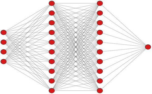
The database was used to build two ML models for the peak HRR prediction. ANNs were used to analyze the behavior of spill fire scenarios. ANNs can consist of billions of neurons that are interconnected with trillions of links. ANNs are modeled after biological neural networks and designed to accomplish specific tasks like classification, regression, and clustering. ANNs, like neural networks, acquire knowledge through training and apply it within the inter-neuron connection strengths, known as weights. A graph represents ANNs with the inputs connected to the first hidden layer, the first hidden layer connected to the second/final hidden layer, and the second/final hidden layer connected to the outputs. Each connection in the graph carries a weight, which represents the strength of the interconnection. The sum of the weighted inputs is passed through an activation function at a neuron. This function produces an output signal and introduces non-linearity in the network. Sigmoidal or logistic, hyperbolic tangent, and rectified linear unit functions are some of the commonly used activation functions. The training of the network employs a set of rules called the learning algorithm. A threshold is applied to the neuron’s response to arrive at the desired value. For a deeper understanding of the ANN method, it can be referred to [26]. Figure 1 displays a fully connected ANN network that has two hidden layers.

Figure 1. Schematic of a fully connected network made with one input and output layer and two hidden layers.

In this study, the spill fire database was utilized to construct Multi-Layer Perceptron (MLP) model, which is a type of ANN for the prediction of peak HRRs of each spill fire scenario. The data is split into a training set (80%), which is used to fit the model parameters that map inputs to outputs, and a test set (20%), which evaluates model performance on separate data to prevent overfitting and ensure generalizability. The machine learning model was developed on the platform of Python 3.6 [27] and TensorFlow 2.0 [28]. To prevent overfitting, k-fold cross-validation was used during the training of the MLP model.

The grid search method was used to find the best hyperparameters that maximize model performance. The ranges of hyperparameters for grid search are the number of hidden layers [2–6], number of neurons [25, 50, 100], and activation function [relu, tanh, sigmoid]. Following a thorough process of optimizing the model structure and hyperparameters, it was concluded that the architecture of the MLP model is 4/50/50/1 for the fixed quantity scenario. The model is trained using an Adam optimizer with a learning rate of 0.001, ‘relu’ activation function, no regularization, and a dropout rate of 0.1 for each layer for a fixed quantity. Similarly, it was concluded that the architecture of the MLP model is 4/100/100/1 for the continuous fed scenario. The model is trained using an Adam optimizer with a learning rate of 0.001, ‘tanh’ activation function, no regularization, and a dropout rate of 0.1 for each layer.

The performance of the trained MLP models according to activation functions, number of hidden layers, and number of neurons in each hidden layer are shown in Table 3. The performance of the trained models is evaluated using root-mean squared error (RMSE) and regression coefficient ($R^2$). As seen in Table 3, the ML models showed good agreement, with low RMSE values and high testing R². These models are used to propagate uncertainties of the input variables.

Table 3. Performances of MLP models for each fire scenario.

Spill Fire Scenario	MLP Structure	Activation Function	Training RMSE [kW]	Testing RMSE [kW]	Training ${\mathit{R}}^2$	Testing ${\mathit{R}}^2$
Fixed Quantity	4/50/50/1	relu	0.031	0.063	0.97	0.94
Continuous Fed	4/100/100/1	tanh	0.044	0.046	0.95	0.87

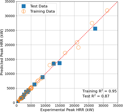
The predicted peak HRR data using MLP models showing best-estimate performance according to hyperparameters tuning results were compared with actual peak HRR data as plotted in Figures 2 and 3. No bias in the prediction was observed against any of the independent variables.

Figure 2. Comparison of predicted peak HRR by MLP and experimentally measured data according to training and testing datasets for fixed quantity spill fire.

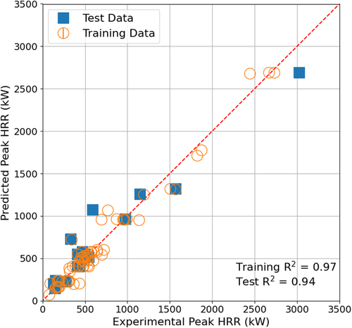
Figure 3. Comparison of predicted peak HRR by MLP and experimentally measured data according to training and testing datasets for continuous fed spill fire.

3. Development of the uncertainty quantification framework

3.1. Characterization of the uncertain parameters

In this section, the Monte Carlo sampling method, which has been predominantly employed in the exploration of uncertainties within fire risk assessment [29,34,35] is utilized to reproduce a probability distribution representing the uncertainties in each input parameter. Tables 4 and 5 display the selected input parameters for the fixed quantity and continuous fed spill fire experiments, along with their corresponding probability distributions and ranges of uncertainty. Normal distributions are used to represent the uncertainty associated with these parameters.

Table 4. Input parameters’ uncertainty range and their characterization for a fixed quantity spill fire scenario.

Parameter	Parameter Range	Parameter Uncertainty*
Fuel Amount Parameter (V)	500–1414 $\mathit{m}{m}^{3/2}$	±2.5% [30]
Ignition Delay Time (IDT)	30–300 second	±5% [30]
Fuel Properties Parameter (MBR/NP)	3.77–10.11 $\mathit{kg}/m^{5/2}$	±8.2% [13]
Substrate Thermal Conductivity (STC)	0.17–1.4 W/m-K	±5% [33]

*Estimated based on the cited references.

Table 5. Input parameters’ uncertainty range and their characterization for continuous fed spill fire scenario.

Parameter	Parameter Range	Parameter Uncertainty*
Slope Angle (S)	0–4 °	±0.01° [18]
Fuel Discharge Rate Parameter (DR)	25–820 $\mathit{m}{m}^{3/2}/s^{1/2}$	±2.5% [31]
Fuel Properties Parameter (MBR/NP)	9.27–18.6 $\mathit{kg}/m^{5/2}$	±8.2% [13]
Substrate Thermal Conductivity (STC)	0.59–35 W/m-K	±5% [33]

*Estimated based on the cited references.

The input parameters for each scenario are simultaneously sampled using the corresponding uncertainty ranges specified in the Dakota input file. Dakota’s preprocessing capability propagates these input parameter uncertainties into the ML predictions. The Dakota master program then automatically launches the UQ calculations, collecting the results of interest after each completed case and proceeding to the next case in line. Once all cases are finished, Dakota generates a result file and performs various statistical analyses using its post-process capability.

It should be noted that most of the collected spill fire experiments did not report experimental data uncertainty. The available literature was reviewed to find appropriated uncertainty ranges for each input parameter assuming a normal distribution [8,34,36–38]. We used our engineering judgement to choose reasonable uncertainty ranges, which involved a detailed review of measurement precision used in the experiments, reported experiment repeatability, and overall variability in parameters across the literature. Also, uncertainty propagation formula was applied for fuel amount parameter, fuel discharge rate parameter, and fuel properties parameter.

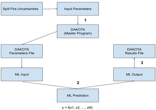
3.2. A framework to couple machine learning to Dakota

A coupling interface developed to connect Dakota and the ML model allows the values of variables determined by Dakota to be transmitted to the ML model and the output of the ML model to be sent back to Dakota. After the necessary simulations are conducted, Dakota produces the results of the uncertainty quantification analysis and the Sobol indices coefficients. The developed framework is named in this work as ‘ML-DAKOTA coupled UQ framework’ and it is presented in Figure 4.

Figure 4. ML-DAKOTA coupled UQ framework.

3.2.1. Variance-based sensitivity analysis

After the uncertainties are propagated through the ML models to predict the peak HRR uncertainty, the mean and the variance are calculated by:

(3) $\mathit{E}\left(\mathit{Y}\right)=\frac{1}{N}\sum y_i$(3)

(4) $\mathit{Var}\left(\mathit{Y}\right)=\frac{1}{\mathit{N}-1}\sum (y_i-\mathit{E}\left(\mathit{Y}\right){)}^2$(4)

The uncertainty in the mean can be estimated, according to the central limit theorem with the following standard error [39]:

(5) $\mathit{SE}\left(\mathit{E}\left(\mathit{Y}\right)\right)=\sqrt{\frac{\mathit{Var}\left(\mathit{Y}\right)}{N}}$(5)

Dakota is employed for the global sensitivity analysis through variance-based decomposition using Sobol’ indices [25,40]. The Sobol’ indices represent a proportion of the output variance, which can be attributed to a specific input parameter alone (referred to as the main effect, S_j), or in conjunction with other input parameters (referred to as the total effect, T_j). These indices provide insight into the relative importance of each input parameter, and their interactions in contributing to the overall variability of the output. Understanding the Sobol’ indices can aid in optimizing the performance of a model or system, by identifying the most influential input parameters, and determining which ones should be prioritized for further analysis or improvement.

The main effect, S_j, and the total effect, T_j, sensitivity indices are represented for a given input parameter X_j and an output of interest Y as:

(6) $S_j=\frac{\mathit{Var}(\mathit{E}(\mathit{Y}|X_j))}{\mathit{Var}\left(\mathit{Y}\right)}$(6)

(7) $T_j=\frac{\mathit{E}(\mathit{Var}(\mathit{Y}|{\mathit{X}}_{\sim \mathit{j})})}{\mathit{Var}\left(\mathit{Y}\right)}$(7)

where E(Y|Xj) is the expected value of Y conditioned on X_j, E(Var(Y|X_~j)) is the expected value of the variance Y conditioned on X_~j and X_~j represents the set of all the input variables except X_j. (⁓j denotes the exception of j parameter from all input parameters). Values vary from 0 to 1: the closer S_j to 1, the higher the contribution of X_j to the uncertainty of the output interest Y and vice versa. The sum of S_j over all input parameters is less than or equal to one. The sum of all the total effects indices may exceed one since some interactions may be counted twice.

3.2.2. Convergence study of sampling size

To determine a suitable sampling size for achieving convergence and accuracy of sensitivity analysis outcomes, we conducted a convergence analysis by altering the sample size for each method and comparing the Sobol indices.

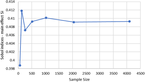
It should be noted that for the sampling size, it is recommended to use $2^N$ [28]. In this study, N ranges from 7 to 12. The sampling size is compared using Sobol indices for both spill fire scenarios. A convergence criterion was set such that the difference in the Sobol indices needs to be less than 0.0005. By increasing the sampling size, the Sobol indices depicted in Figure 5, ultimately converge at 2048 samples. Therefore, 2048 samples are generated in Monte Carlo analysis for uncertainty quantification and sensitivity analysis.

Figure 5. Convergence study of Sobol indices representing the main effect for the fixed quantify dataset.

4. Performance of uncertainty framework

4.1. Uncertainty quantification results

One of the current challenges in using machine learning is to evaluate the uncertainty associated with the predictions made by the developed models. To evaluate the framework’s performance, the test set containing 17 data points for each spill fire scenario was initially analyzed. The mean and standard deviation of the predicted peak HRRs were calculated for each test case. Tables 6 and 7 summarize these statistical moments for the fixed quantity and continuous fed scenarios, respectively. A Kolmogorov–Smirnov test [41] was used to validate the normality assumption of peak HRR distributions for all data points in Tables 6 and 7 with a 95% confidence. Experiments with a higher coefficient of variation indicate greater relative variability in the model’s HRR estimates compared to the actual value. Tables 6 and 7 show a maximum coefficient of variation of 25.3% and 28.3% for data points 9 and 3, respectively.

Table 6. Moments of peak HRR for 17 experimental data (fixed quantity).

Experiment No	V ($\mathit{m}{m}^{3/2})$	IDT (second)	MBR/NP ($\mathit{kg}/m^{5/2})$	STC (W/m-K)	Mean Peak HRR (kW)	STD (kW)	Coefficient of variation (%)
1 [31]	707.1	30	10.11	1.4	485.9	29.9	6.2
2 [31]	1000	30	10.11	1.4	965.3	74.1	7.7
3 [31]	1000	300	10.11	1.4	484.4	47.6	9.8
4 [31]	707.1	300	18.6	1.4	204.9	33.5	16.4
5 [31]	1000	30	18.6	1.4	1194.8	112.1	9.4
6 [31]	1000	300	18.6	1.4	548.4	58.2	10.6
7 [31]	707.1	30	3.77	1.4	147.9	28.5	19.3
8 [31]	1000	30	3.77	1.4	322.3	32.8	10.2
9 [31]	1000	300	3.77	1.4	227.7	57.7	25.3
10 [31]	707.1	300	10.11	1.4	246.5	31.1	12.6
11 [31]	707.1	30	10.11	1.4	485.9	29.9	6.2
12 [32]	1000	30	10.11	0.19	1320.3	137.7	10.4
13 [32]	1000	30	3.77	0.19	499.4	93.3	18.7
14 [32]	707.1	30	10.11	0.17	586.1	98.6	16.8
15 [32]	707.1	30	6.91	0.17	527.8	90.4	17.1
16 [32]	1414.2	30	10.11	0.19	2651.3	524.2	19.8
17 [33]	1000	150	10.11	0.19	1554.2	256.1	16.4

Table 7. Moments of peak HRR for 17 experimental data (continuous fed).

Experiment No	S (°)	DR ($\mathit{m}{m}^{3/2}/s^{1/2})$	MBR/NP ($\mathit{kg}/m^{5/2})$	STC (W/m-K)	Mean Peak HRR (kW)	STD (kW)	Coefficient of variation (%)
1 [16]	0	184.86	9.53	1.5	1696.4	172.8	10.1
2 [16]	0	270.52	9.53	1.5	4291.1	706.5	16.4
3 [16]	0	124.51	18.6	1.5	1544.9	436.2	28.3
4 [16]	0	184.86	18.6	1.5	2777.5	253.4	9.1
5 [16]	0	337.18	18.6	1.5	6294.7	974.3	15.4
6 [20]	0	223.98	9.27	1.5	3723.2	606.5	16.2
7 [20]	0.5	184.84	9.27	1.5	2012.2	366.1	18.1
8 [20]	0.5	223.98	9.27	1.5	3696.3	703.8	19.0
9 [20]	1	223.98	9.27	1.5	3809.7	602.9	15.8
10 [21]	0	586.52	18.6	0.59	25571.3	5720.1	22.3
11 [21]	0	254.95	18.6	0.59	13696.4	1891.6	13.8
12 [17]	0	58.48	18.6	1.5	165.1	14.9	9.0
13 [17]	0	87.06	18.6	1.5	314.3	34.6	11.0
14 [21]	0	500	18.6	0.59	13499.4	2786.3	20.6
15 [14]	0	60.28	18.6	0.59	398.1	63.8	16.0
16 [18]	1	184.84	18.6	1.5	3742.5	686.5	18.3
17 [18]	3	299.72	18.6	1.5	8873.0	1662.9	18.7

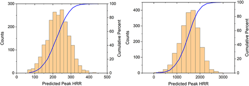
The peak HRR distributions are shown in Figure 6, it provides visual representations of the predicted HRR distribution for two experiments, offering insights into the range and variability of HRR values as estimated by the model. Experiment 9 has a mean value of 227.7 kW and a standard deviation of 57.7 kW. The 95% confidence bound is 231.47 kW, representing a 10.3 kW deviation from the experimental peak HRR value of 241.8 kW. Experiment 3 has a mean value of 1544.9 kW and a standard deviation of 436.2 kW. The 95% confidence bound value is 1560.9 kW, representing a 17.5 kW deviation from the experimental peak HRR value of 1543.4 kW.

Figure 6. MLP predicted peak HRR distribution (exp. 9-left and exp.3-right).

The overall uncertainties are shown in Figures 7–10 with 95% confidence intervals compared to the data distribution. In Figure 7, as fuel amount parameter increases, the peak HRR grows nonlinearly. Confidence interval widths at higher fuel quantities are larger due to the limited number of data points as the volume parameter increases. In other words, the non-linearity of MLP models allows for the uncertainty of the model to increase in the regions where a limited or absence of data exists.

Figure 7. Peak HRR predictions with 95% CIs vs. fuel amount parameter (fixed quantity spill fire). Fuel amount parameter distribution shown at bottom right.

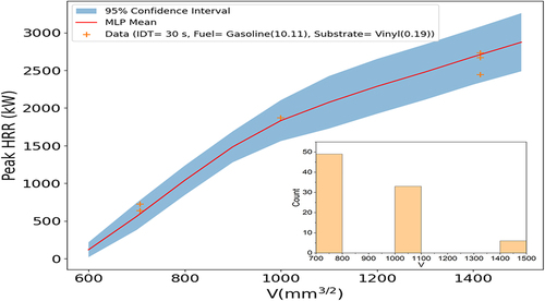
Figure 8. Peak HRR predictions with 95% CIs vs. fuel amount for 30- and 150-sec IDTs (fixed quantity spill fire). IDT distribution shown at bottom right.

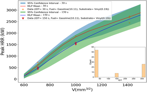
Figure 9. Peak HRR predictions with 95% CIs vs. fuel amount for heptane and gasoline (fixed quantity spill fire). MBR/NP distribution shown at top left.

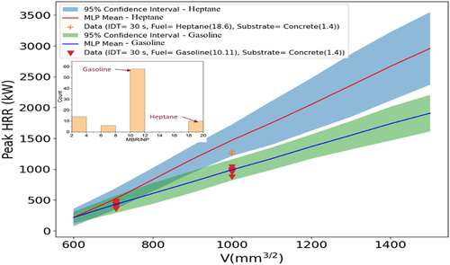
Figure 10. Peak HRR predictions with 95% CIs vs. fuel amount for vinyl and concrete (fixed quantity spill fire). STC distribution shown at bottom right.

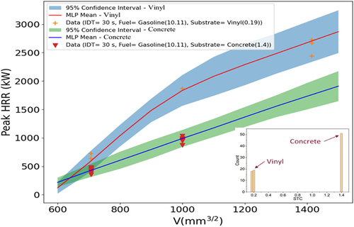
Similarly, Figure 8 shows the winder confidence bands at higher delay times where input data are scarcer, as shown in the IDT distribution. Figure 9 reveals larger uncertainty for heptane relative to gasoline, as the training data are sparser for heptane. Figure 10 exhibits peak HRR prediction with 95% confidence band for vinyl and concrete substrates. The substrate data distribution indicates there is a lack of vinyl data. Therefore, the uncertainty bands grow wider for vinyl, reflecting greater uncertainty with less data.

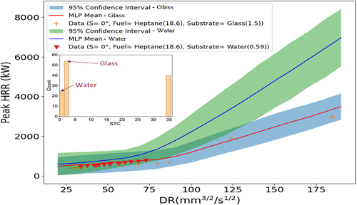
The same analysis was performed for the continuous fed spill fires, as shown in Figures 11–14 for the peak heat HRR predictions with 95% confidence intervals across various conditions. The uncertainty bands widen in regions where experimental data are sparser, reflecting greater uncertainty in the model predictions. Specifically, the discharge rate parameter and slope angle distributions (Figures 11 and 12) indicate that data are scarcer at higher values, leading to expanded uncertainty bands in those regimes. Furthermore, the fuel type and substrate distributions (Figures 13 and 14) reveal wider confidence intervals for JP-4 fuel and water substrate, for which less data are available compared to heptane and glass. The uncertainty quantification highlights areas where collecting additional empirical evidence would enhance model robustness. This analysis provides data-driven insights to guide future experimental efforts toward regimes that can augment model predictive capabilities.

Figure 11. Peak HRR predictions with 95% CIs vs. discharge rate parameter (continuous fed spill fire). Discharge rate parameter distribution shown at bottom right.

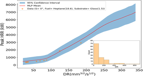
Figure 12. Peak HRR predictions with 95% CIs vs. discharge rate parameter (continuous fed spill fire) for 0° and 3°. Slope angle distribution shown at top left.

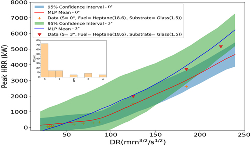
Figure 13. Peak HRR predictions with 95% CIs vs. discharge rate parameter (continuous fed spill fire) for heptane and JP-4. Fuel parameter distribution shown at top left.

Figure 14. Peak HRR predictions with 95% CIs vs. discharge rate parameter (continuous fed spill fire) for glass and water. Substrate distribution shown at top left.

4.2. The results of Sobol indices

The contribution of each parameter in the overall performance of the model is shown in Table 8 and Figure 15 through the Sobol indices for both the total effect and main effect in the spill fire scenarios. Notably, for the fixed quantity scenario, the fuel amount parameter accounts for 54.4% of variance in peak HRR as the primary contributor, while the fuel properties parameter explains 22.6% of the variance. In comparison, ignition delay time and substrate thermal conductivity play a smaller role, contributing 8.09% and 9.45% to the output variance, respectively. Additionally, it is observed that the sum of the main effect indices does not surpass 95%. This implies that the interactions between the input parameters have a relatively minor impact, representing approximately 5% of the output variance.

Figure 15. Sobol indices the main and the total effects of the studied parameters based on 2048 samples for fixed quantity spill fire scenario based on Table 8 data.

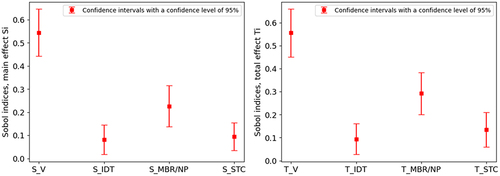
Table 8. Sobol indices of the key parameters of spill fire peak HRR model for test data (fixed quantity spill fire scenario).

Parameter	Total Effect Ti	Main Effect Si
Fuel amount Parameter (V)	0.555 ± 0.1035	0.544 ± 0.102
Ignition Delay Time (IDT)	0.0934 ± 0.067	0.0809 ± 0.0639
Fuel Properties Parameter (MBR/NP)	0.292 ± 0.0915	0.226 ± 0.089
Substrate Thermal Conductivity (STC)	0.134 ± 0.075	0.0945 ± 0.0604
Total	0.05	0.95

Table 9 and Figure 16 present the Sobol indices of the total effect and main effect, for continuous fed spill fire. Notably, the fuel discharge rate parameter accounts for a substantial 41.8% of the variance in peak HRR as the foremost contributing factor. Meanwhile, the fuel properties parameter explains 39.3% of the variance as the second most influential parameter. In contrast, the slope angle and substrate thermal conductivity have small impacts, contributing only less than 0.1% and 18.6% to the output variance, respectively. Additionally, it is observed that the sum of the main effect indices does not surpass 99%. This implies that the interactions between the input parameters have a relatively minor impact, representing approximately 1% of the output variance. Overall, the sensitivity analysis quantitatively identifies the most influential input parameters contributing to uncertainty in predicting peak HRRs for both fixed quantity and continuous fed spill fire scenarios, providing data-driven insights to guide targeted data collection efforts.

Figure 16. Sobol indices the main and the total effects of the studied parameters based on 2048 samples for continuous fed spill fire scenario based on Table 9 data.

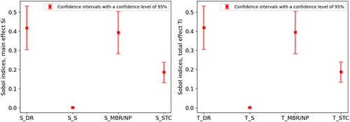
Table 9. Sobol indices of the key parameters of spill fire peak HRR model for test data (continuous fed spill fire scenario).

Parameter	Total Effect Ti	Main Effect Si
Fuel Discharge Rate Parameter (DR)	0.418 ± 0.1135	0.418 ± 0.114
Slope Angle (S)	2.647E–4 ± 7.41E–5	2.547E–4 ± 7.485E–5
Fuel Properties Parameter (MBR/NP)	0.394 ± 0.112	0.393 ± 0.1105
Substrate Thermal Conductivity (STC)	0.187 ± 0.053	0.186 ± 0.053
Total	0.01	0.99

5. Conclusion

This study presents a novel framework integrating Monte Carlo and ANN to quantify sources of uncertainty in modeling unconfined spill fire scenarios, and to obtain low-order statistics representing the average quantities of interest. To achieve this, an experimental database is utilized to train and validate the ANN algorithm. Besides, various parameters in the model are systematically varied to align with values reported in existing literature.

This work investigates two sources of uncertainty that impact the peak HRR prediction using the ANN spill fire model, which are lack of data and input parameters.

The UQ analysis reveals important insights into the impact of data scarcity on the prediction reliability with the use of ANN methods. The analysis has shown that the confidence intervals widen at higher fuel quantities and ignition delay time (fixed quantity spills), discharge rates and slope angles (continuous fed spills), where data are scarcer. In addition, the lack of data has caused similar impact on the widening of the confidence intervals, when different materials (fuel or substrate) are compared against each other, such as the fixed quantity case where gasoline data produce better UQ evaluation accuracy compared to the heptane data.

Sensitivity analysis results reveal that certain key parameters significantly influence the peak HRR predictions in both fixed quantity and continuous fed spill fire scenarios. For the fixed quantity scenario, the fuel amount parameter accounts for 54.4% of variance in peak HRR as the primary contributor, while the fuel properties parameter explains 22.6% of the variance. For the continuous fed scenario, the fuel discharge rate parameter accounts for a substantial 41.8% of the variance in peak HRR as the foremost contributing factor, followed by the fuel properties parameter accounts for 39.3% of the variance.

To summarize, the presented framework provides data-driven insights to guide targeted data collection efforts, due to uncertainty from limited data, and quantitatively identifies the most influential input parameters contributing to uncertainty in predicting peak HRRs for spill fires. This work can be utilized in the development of more advanced ANN models for predicting the peak HRR values of spill fire scenarios, ultimately reducing the uncertainties in fire risk parameters, such as severity factor calculation, zone of influence, and target damage analysis especially in NPPs, and optimizing resources allocation in the future research.

While this work focuses on modeling peak HRR for liquid fuel spill fires, the framework will be extended to assess fire risk from electrical cables and enclosures, which are prevalent fire initiation points in fire PRA for NPPs. Future efforts will apply similar data-driven techniques to build predictive models for cable-based and electrical cabinet fire scenarios.

Nomenclature

$\mathit{DR}$	=	discharge rate parameter, square root of the discharge rate, $\left({\left(m{m}^3/\mathit{s}\right)}^{1/2}\right)$
$\mathit{IDT}$	=	ignition delay time $\left(\mathrm{seconds}\right)$
$\mathit{HRR}$	=	heat release rate $\left(\mathrm{kW}\right)$
$\mathit{MBR}/\mathit{NP}$	=	fuel properties parameter $(\mathit{kg}/m^{5/2}$]
${\dot{m}}_{\mathrm{\infty }}^{{ }^{\prime \prime }}$	=	maximum mass burning rate per unit area $\left(\mathit{kg}/m^2.\mathit{s}\right)$
$\mathit{S}$	=	slope angle $\left({ }^{\circ }\right)$
$\mathit{STC}$	=	substrate thermal conductivity $(\mathit{W}/\mathit{m}.\mathit{K})$
$\mathit{V}$	=	fuel quantity parameter, square root of fuel quantity, $\left(\mathit{m}{m}^{3/2}\right)$
Greek Symbols	=
$\mathit{\delta }$	=	fuel thickness $\left(\mathit{mm}\right)$
ρ	=	density $\left(\mathit{kg}/m^3\right)$
$\mathit{\sigma }$	=	surface tension $\left(\mathit{N}/\mathit{m}\right)$
Acronyms	=
ANN	=	artificial neural network
MLP	=	multilayer perceptron
NPP	=	nuclear power plant
SFPE	=	society of fire protection engineers

Acknowledgments

The research was funded through the U.S. Department of Energy, Office of Nuclear Energy through Award No. DE-NE0008981. Elvan Sahin is also supported by the Turkish Ministry of National Education for his PhD studies.

Disclosure statement

No potential conflict of interest was reported by the author(s).

Additional information

Funding

The work was supported by the Nuclear Energy University Program [DE-NE0008981]; Turkish Ministry of National Education.

References

- Salvi U, Lattimer BY, Alhadhrami S, et al. Analysis of historic fires to determine most frequent challenging events. Prog Nucl Energy. 2022;146:104146. doi: 10.1016/j.pnucene.2022.104146
- Sahin E, Salvi U, Wang J, et al. Assessment of fire experimental data for use in nuclear power plants fire PRA. Americal Nuclear Society (ANS) 2022 Annual Meeting. 2022;126:504–507.
- Siu NO. Physical models for compartment fires. Reliab Eng. 1982;3(3):229–252. doi: 10.1016/0143-8174(82)90032-4
- Siu NO, Apostolakis GE. Probabilistic models for cable tray fires. Reliab Eng. 1982;3(3):213–227. doi: 10.1016/0143-8174(82)90031-2
- Ho VS, Siu NO, Apostolakis G, et al. COMPBRN III: a computer code for modeling compartment fires; 1986. ( NUREG/CR-4566, ORNL/TM-10005).
- Ho V, Siu N, Apostolakis G. COMPBRN III—A fire hazard model for risk analysis. Fire Saf J. 1988;13(2–3):137–154. doi: 10.1016/0379-7112(88)90009-4
- Holborn PG, Nolan PF, Golt J. An analysis of fire sizes, fire growth rates and times between events using data from fire investigations. Fire Saf J. 2004;39(6):481–524. doi: 10.1016/j.firesaf.2004.05.002
- Au SK, Wang Z-H, Lo S-M. Compartment fire risk analysis by advanced Monte Carlo simulation. Eng Struct. 2007;29(9):2381–2390. doi: 10.1016/j.engstruct.2006.11.024
- Jin Y, Bajorek SM, Cheung F-B. Validation and uncertainty quantification of transient reflood models using COBRA-TF and machine learning techniques based on the NRC/PSU RBHT Benchmark. Nucl Sci Eng. 2023;197(5):967–986. doi: 10.1080/00295639.2022.2087834
- Brandyberry M, Apostolakis G. Response surface approximation of a fire risk analysis computer code. Reliab Eng Syst Saf. 1990;29(2):153–184. doi: 10.1016/0951-8320(90)90077-Z
- Worrell C, Luangkesorn L, Haight J, et al. Machine learning of fire hazard model simulations for use in probabilistic safety assessments at nuclear power plants. Reliab Eng Syst Saf. 2019;183:128–142. doi: 10.1016/j.ress.2018.11.014
- Sahin E, Lattimer BY, Duarte JP. Assessing spill fire characteristics through machine learning analysis. Ann Nucl Energy. 2023;192:109961. doi: 10.1016/j.anucene.2023.109961
- Hurley MJ, Gottuk DT, Hall JR Jr, et al. SFPE handbook of fire protection engineering. New York, Heidelberg, Dordrecht, London: Springer; 2015.
- Li Y, Huang H, Zhang J, et al. Large-scale experimental study on the spread and burning behavior of continuous liquid fuel spill fires on water. J Fire Sci. 2014;32(5):391–405. doi: 10.1177/0734904114526956
- Li Y, Huang H, Shuai J, et al. Experimental study of continuously released liquid fuel spill fires on land and water in a channel. J Loss Prevent Process Indust. 2018;52:21–28. doi: 10.1016/j.jlp.2018.01.008
- Zhao J, Liu Q, Huang H, et al. Experiments investigating fuel spread behaviors for continuous spill fires on fireproof glass. J Fire Sci. 2017;35(1):80–95. doi: 10.1177/0734904116683716
- Zhao J, Zhu H, Huang H, et al. Experimental study on the liquid layer spread and burning behaviors of continuous heptane spill fires. Process SafEnviron Prot. 2019;122:320–327. doi: 10.1016/j.psep.2018.12.021
- Liu Q, Zhao J, Lv Z, et al. Experimental study on the effect of substrate slope on continuously released heptane spill fires. J Therm Anal Calorim. 2020;140(5):2497–2503. doi: 10.1007/s10973-019-08998-9
- Li Y, Huang H, Zhang L, et al. An experimental investigation into the effect of substrate slope on the continuously released liquid fuel spill fires. J Loss Prevent Process Indust. 2017;45:203–209. doi: 10.1016/j.jlp.2017.01.010
- Zhao J, Zhu H, Zhang J, et al. Experimental study on the spread and burning behaviors of continuously discharge spill fires under different slopes. J Hazard Mater. 2020;392:122352. doi: 10.1016/j.jhazmat.2020.122352
- Li Y, Huang H, Wang Z, et al. An experimental and modeling study of continuous liquid fuel spill fires on water. J Loss Prevent Process Indust. 2015;33:250–257. doi: 10.1016/j.jlp.2015.01.006
- Li H, Liu H, Liu J, et al. Spread and burning characteristics of continuous spill fires in a tunnel. Tunn Undergr Space Technol. 2021;109:103754. doi: 10.1016/j.tust.2020.103754
- Li Y, Meng D, Yang L, et al. Experimental study on the burning rate of continuously released spill fire on open surface with measurement of burning fuel thickness. Case Stud Thermal Eng. 2022;36:102217. doi: 10.1016/j.csite.2022.102217
- Sobol’ IM. On sensitivity estimation for nonlinear mathematical models. Matematicheskoe modelirovanie. 1990;2:112–118.
- Dalbey K, Eldred MS, Geraci G, et al. Dakota a multilevel parallel object-oriented framework for design optimization parameter estimation uncertainty quantification and sensitivity analysis: version 6.12 theory manual [internet]. Sandia National Lab. (SNL-NM), Albuquerque, NM (United States); 2020 [cited 2023 Apr 23]. Report No.: SAND-2020-4987. https://www.osti.gov/biblio/1630693.
- Kotteda VMK, Stephens JA, Spotz W, et al. Uncertainty quantification of fluidized beds using a data-driven framework. Powder Technol. 2019;354:709–718. doi: 10.1016/j.powtec.2019.06.021
- van Rossum G, Drake FL. Python reference manual.
- Pedregosa F, Varoquaux G, Gramfort A, et al. Scikit-learn: machine learning in Python. J Mach Learn Res. 2011;12:2825–2830.
- Brandyberry MD, Apostolakis GE. Fire risk in buildings: frequency of exposure and physical model. Fire Saf J. 1991;17(5):339–361. doi: 10.1016/0379-7112(91)90017-S
- Benfer ME, Professor JLB, Quintiere JG. Spill and burning behavior of flammable liquids [master’s thesis]. University of Maryland; 2010.
- Mealy CL, Benfer ME, Gottuk DT. Fire Dynamics and Forensic Analysis of Liquid Fuel Fires. 2012. 237.
- Mealy CL, Gottuk DT. Ignitable liquid fuel fires in buildings – a study of fire dynamics. 2013. 179.
- Jr ADP, McElroy JA, Madrzykowski D. Flammable and Combustible Liquid Spill/Burn Patterns (NIJ Report 604-00). 2001;53.
- Brandyberry MD, Apostolakis GE. Fire risk in buildings: scenario definition and ignition frequency calculations. Fire Saf J. 1991;17(5):363–386. doi: 10.1016/0379-7112(91)90018-T
- Phillips WGB. Simulation models for fire risk assessment. Fire Saf J. 1994;23(2):159–169. doi: 10.1016/0379-7112(94)90023-X
- Frantzich H, Kazunori H. Uncertainty analysis and safety verification. Fire safety design based on calculations. 1995.
- Frantzich H. Risk analysis and fire safety engineering. Fire Saf J. 1998;31(4):313–329. doi: 10.1016/S0379-7112(98)00021-6
- Iooss B, Lemaître P. A review on global sensitivity analysis methods. Uncertainty management in simulation-optimization of complex systems: algorithms and applications. 2015. 101–122.
- Saltelli A, Ratto M, Andres T, et al. Global Sensitivity Analysis. The Primer [Internet]. 1st ed. Wiley. 2007 [cited 2023 Apr 26]. https://onlinelibrary.wiley.com/doi/book/10.1002/9780470725184.
- Sobol′ IM. Global sensitivity indices for nonlinear mathematical models and their Monte Carlo estimates. Math Comput Simul. 2001;55(1–3):271–280. doi: 10.1016/S0378-4754(00)00270-6
- Massey FJ. The Kolmogorov-Smirnov test for goodness of fit. J Am Stat Assoc. 1951;46(253):68–78. doi: 10.1080/01621459.1951.10500769