Heat of transport for hydrogen and hydrides in Zircaloy

ABSTRACT

Hydrogen diffuses in zirconium alloys in response to gradients in hydrogen concentration, temperature, and stress. This essay discusses the results of several evaluations of the coefficient describing the effects of temperature gradients called the heat of transport. The values distinguish between when hydrogen is in solution, (25 ± 3) kJ/mol, and when stable hydrides are present, (116 ± 17) kJ/mol.

KEYWORDS:

• Heat of transport
• Zircaloy
• hydrogen migration
• hydride diffusion
• Bison

1. Introduction

The flux, J, of atomic hydrogen in solid solution in zirconium is determined by gradients in hydrogen concentration, stress, temperature, and alloy composition (the latter is not considered here):

(1) $\mathrm{J}=-\mathit{D}\left(\mathrm{\nabla C}+\frac{\mathit{CV}}{\mathit{RT}}\mathrm{\nabla \sigma }+\frac{C{Q}^{\ast }}{\mathit{R}{T}^2}\mathrm{\nabla T}\right).$(1)

D is the diffusivity of hydrogen in zirconium, R is the Gas Constant, T the temperature, V is the partial molar volume of hydrogen in Zircaloy, σ is the hydrostatic stress experienced by a hydrogen atom in solid solution surrounded by the crystal lattice. The first term in Equation 1(1) $\mathrm{J}=-\mathit{D}\left(\mathrm{\nabla C}+\frac{\mathit{CV}}{\mathit{RT}}\mathrm{\nabla \sigma }+\frac{C{Q}^{\ast }}{\mathit{R}{T}^2}\mathrm{\nabla T}\right).$(1) is the Fick’s Law current; the second term is the drift current; these terms can be derived from the chemical potential of hydrogen in solid solution [1], in which case C is the concentration of hydrogen in solid solution. The flux in Equation 1(1) $\mathrm{J}=-\mathit{D}\left(\mathrm{\nabla C}+\frac{\mathit{CV}}{\mathit{RT}}\mathrm{\nabla \sigma }+\frac{C{Q}^{\ast }}{\mathit{R}{T}^2}\mathrm{\nabla T}\right).$(1) is equal to the concentration of hydrogen in solution multiplied by the terminal velocity of hydrogen atoms that is proportional to a force written as the negative gradient of the chemical potential of hydrogen in solution that includes a term to account for the local work done by the solute (i.e., hydrogen in solution) to expand the lattice of the metal solvent at constant temperature, i.e., σV. The proportionality constant is the mobility, Γ, which equals D/RT [2]. Equation 1(1) $\mathrm{J}=-\mathit{D}\left(\mathrm{\nabla C}+\frac{\mathit{CV}}{\mathit{RT}}\mathrm{\nabla \sigma }+\frac{C{Q}^{\ast }}{\mathit{R}{T}^2}\mathrm{\nabla T}\right).$(1) is not limited to hydrogen in solution: because the chemical potentials of hydrogen in all forms in the metal must be equal when J = 0. Equation 1(1) $\mathrm{J}=-\mathit{D}\left(\mathrm{\nabla C}+\frac{\mathit{CV}}{\mathit{RT}}\mathrm{\nabla \sigma }+\frac{C{Q}^{\ast }}{\mathit{R}{T}^2}\mathrm{\nabla T}\right).$(1) will also work when hydrides are present, in which case C is the total concentration of hydrogen in the specimen. Equation 1(1) $\mathrm{J}=-\mathit{D}\left(\mathrm{\nabla C}+\frac{\mathit{CV}}{\mathit{RT}}\mathrm{\nabla \sigma }+\frac{C{Q}^{\ast }}{\mathit{R}{T}^2}\mathrm{\nabla T}\right).$(1) is general and can be applied to any quantifiable objects that move according to forces that derive from gradients in concentration, stress, and temperature.

The third term in Equation 1(1) $\mathrm{J}=-\mathit{D}\left(\mathrm{\nabla C}+\frac{\mathit{CV}}{\mathit{RT}}\mathrm{\nabla \sigma }+\frac{C{Q}^{\ast }}{\mathit{R}{T}^2}\mathrm{\nabla T}\right).$(1) is the Soret current that arises from a temperature gradient. When hydrogen moves from a high to low temperature region in the metal, the hot hydrogen loses kinetic energy to the cold lattice; the energy lost is the heat of transport. In this case, an entropy term equal to S∇T is added to the gradient of Gibb’s free energy, where S is the entropy of transfer, i.e., the entropy lost by the region from which the hydrogen left, is equal to the heat transferred by transporting hydrogen divided by the temperature [3]. The lower the temperature the higher the entropy, so hydrogen is driven to cooler regions by an increasingly higher rate of entropy production. In units of chemical potential, this temperature-gradient term becomes (Q*/T) ∇T where Q* is the heat of transport in units of J/mol. The negative of this temperature-gradient term is the force that causes hydrogen to move and when multiplied by the mobility and the concentration results in a conjugate flux. Converting mobility to diffusivity as before results in the Soret current in Equation 1(1) $\mathrm{J}=-\mathit{D}\left(\mathrm{\nabla C}+\frac{\mathit{CV}}{\mathit{RT}}\mathrm{\nabla \sigma }+\frac{C{Q}^{\ast }}{\mathit{R}{T}^2}\mathrm{\nabla T}\right).$(1) . The total flux is a superposition of these three independent currents.

For one-dimensional steady-state diffusion (i.e., non-zero gradients and J = 0) and using d/dx = (d/dT)(dT/dx), solving for Q* in Equation 1(1) $\mathrm{J}=-\mathit{D}\left(\mathrm{\nabla C}+\frac{\mathit{CV}}{\mathit{RT}}\mathrm{\nabla \sigma }+\frac{C{Q}^{\ast }}{\mathit{R}{T}^2}\mathrm{\nabla T}\right).$(1) yields for non-zero temperature gradients:

(2) $Q^{\ast }=-\frac{R{T}^2}{\mathit{C}}\left(\frac{\mathit{dC}}{\mathit{dT}}+\frac{\mathit{CV}}{\mathit{RT}}\frac{\mathit{d\sigma }}{\mathit{dT}}\right),$(2)

where the concentration, temperature, and the derivatives are the values at the point of steady state; concentration varies linearly over the temperatures of these experiments. Starting from an initial constant spatial concentration of hydrogen and a positive linear temperature gradient it will be seen that there is an apparent angular velocity associated with ‘clockwise’ rotation of the concentration-temperature profile about a steady-state point that will be limited by the terminal velocity of hydrogen in solution in the coldest region. Thus, the rotation will reach a terminal ‘angular velocity’ and the concentrations will vary linearly with temperature. Hydrogen atoms moving in a line towards the cold end of a specimen can only step forward as fast as the hydrogen atom directly in front steps, so they move in unison, in lockstep, at the terminal velocity of the coldest, and slowest, atoms; the atoms in line neither bunch, nor spread out, so that the concentration varies linearly along the line with temperature.

In a recent paper, Kang et al. [4], described experiments to determine the heat of transport of hydrogen in Zircaloy-4 to support the development of the Bison computer code being developed at Idaho National Laboratory used to predict the redistribution of hydrogen in Zircaloy-4 nuclear fuel cladding because of temperature gradients developed during reactor operation. The experiments started with uniform concentrations of hydrogen in solution in 4 cm length specimens that were subsequently annealed under fixed linear temperature gradients over a range of temperatures. The experiments of Kang et al. were like those reported by Sawatzky in 1960 [5]. The determined heat of transport was for hydrogen moving in solution where no stable hydrides were present. The current paper extends this analysis to include stable hydrides, which may be the case of most practical interest because hydrides are brittle precipitates that have led to fracture of components made from zirconium alloys [6–10]. All the experimental data presented in this paper were reported by others, we analyze their data in a different way. For the calculations that follow, it is assumed that the durations of these experiments were sufficient for the flux to be zero.

2. Heat of transport for hydrogen in solution in Zircaloy-4

As an example of using Equation 2(2) $Q^{\ast }=-\frac{R{T}^2}{\mathit{C}}\left(\frac{\mathit{dC}}{\mathit{dT}}+\frac{\mathit{CV}}{\mathit{RT}}\frac{\mathit{d\sigma }}{\mathit{dT}}\right),$(2) , consider the plots shown in Figure 1 based on data from Sawatzky (figure 2 in [5]) and a plot for experiment UM13 from Kang et al. [4]. The coordinates of the steady-state point for each plot are given by the intersection of the dotted lines in Figure 1; the one-sigma errors are determined from the 95% confidence intervals. Substituting these values into Equation 2(2) $Q^{\ast }=-\frac{R{T}^2}{\mathit{C}}\left(\frac{\mathit{dC}}{\mathit{dT}}+\frac{\mathit{CV}}{\mathit{RT}}\frac{\mathit{d\sigma }}{\mathit{dT}}\right),$(2) yields Q* = (26 ± 4) kJ/mol for the experimental results shown in Figure 1. The contribution of the stress term is small, amounting to less than 1 kJ/mol, which is within the error of the determined values of Q*. The hydrostatic stress is assumed proportional to the yield strength, and the proportionality constant is K which is a sink-strength stress concentration factor [12]. For hydrogen clouds forming in solution, K is assumed to be equal to 1. For Zircaloy-4 and the temperatures used in these experiments, 550 to 860 K, the change of yield strength with temperature is about 0.6 MPa/K [13]. See figure 9.257 in [14] for another example of hydrogen moving where the stress gradient contribution is small compared with the temperature gradient contribution.

Figure 1. The concentration profile produced with linear temperature gradients along a 2.5-cm specimen of Zircaloy-2 after 44 days (left plot) [5], and along a 4 cm Zircaloy-4 specimen after 27 days (right plot) [4]. The steady-state concentrations (i.e., the midpoint of the linear range, C_m) and corresponding temperatures, T_m, are shown by the horizontal and vertical dotted lines; the initial horizontal profile is envisioned to rotate clockwise about this stationary point until J = 0; the results are the plotted measured final profiles. The 95% confidence intervals are shown by the grey curves on either side of the fitted straight line. The dashed red curve in the upper left corners of each plot is C- determined from Equation (3) with the parameters for Zircaloy in [11]; all concentrations are below C- in this experiment so no stable hydrides are present.

Ten experiments reported in [4] were analysed for Q*, these results are shown in Figure 1 to 3. The average value of Q* calculated from these ten experiments is (25 ± 3) kJ/mol. The steady-state point coordinates were calculated from the middle values of concentrations and temperatures for the range where concentration and temperature were linearly related. The final profile depends only on the total concentration, not the initial distribution, so the same final concentration gradient can be envisioned to result from clockwise rotation about a steady-state point defined by the middle values of concentration and temperature. The rotation about this stationary point will be clockwise if the temperature gradient is positive. The value of Q* determined for hydrogen moving in solution with no stable hydrides present using Equation 2(2) $Q^{\ast }=-\frac{R{T}^2}{\mathit{C}}\left(\frac{\mathit{dC}}{\mathit{dT}}+\frac{\mathit{CV}}{\mathit{RT}}\frac{\mathit{d\sigma }}{\mathit{dT}}\right),$(2) is the same as the value recommended by Sawatzky (i.e., 6 kcal/mol = (25 ± 4) kJ/mol [5]) that is currently used in the Bison code [4], and this value of Q* is within error of the value determined by Kang et al. for these same data. In these earlier determinations of Sawatzky, and Kang et al., Equation 2(2) $Q^{\ast }=-\frac{R{T}^2}{\mathit{C}}\left(\frac{\mathit{dC}}{\mathit{dT}}+\frac{\mathit{CV}}{\mathit{RT}}\frac{\mathit{d\sigma }}{\mathit{dT}}\right),$(2) was written as

(3) $Q^{\ast }=\mathit{R}\frac{\mathit{d}ln\mathit{C}}{\mathit{d}\left(1/T\right)}-\mathit{VT}\frac{\mathit{d\sigma }}{\mathit{dT}},$(3)

Figure 3. Experiments [4] demonstrating the departure from the linear concentration dependence with temperature seen at higher temperatures when low temperature concentrations are above C- shown by the dashed red curves in the upper left corner of each plot [11]. Hydrides are present for concentrations above C-. The intersection of the dotted lines shows the point of steady state.

Figure 2. Experiments demonstrating linear concentration dependences with temperature [4]. The intersection of the dotted lines shows the point of steady state. The dashed red curves in the upper left corner of each plot show C- [11]. For these experiments, concentrations below C- indicate no stable hydrides present.

but without the drift term contribution so that the slope of a plot of the logarithm of the concentration versus the reciprocal temperature multiplied by the gas constant approximates the heat of transport. The plot is not a straight line (see the Arrhenius plots in [4]); the slope needs to be evaluated at the stationary point representing steady state and an appropriate tangent can be difficult to define precisely from limited data thus it would seem to be better to use Equation 2(2) $Q^{\ast }=-\frac{R{T}^2}{\mathit{C}}\left(\frac{\mathit{dC}}{\mathit{dT}}+\frac{\mathit{CV}}{\mathit{RT}}\frac{\mathit{d\sigma }}{\mathit{dT}}\right),$(2) to evaluate Q*.

3. Heat of transport for hydrogen in solution and as hydrides in Zircaloy-4

When stable hydrides are present, that is when the concentration of hydrogen in solution in the bulk matrix exceeds C- [1,12] as described later in the Discussion, the slopes of the concentration-temperature plots change. Experiments UM8, UM9, and UM10 (Figure 3) show when the concentration in solution exceeds C- that the linear concentration-temperature dependence changes slope becoming more negative. Similar slope changes were reported by Sawatzky, see figures 4 and 5 in [5] and by Kammenzind et al., see figure 24 in [15] and by Merlino, see figures 10 to 15 in [16]. The change in slope is associated with hydrides.

Equation 2(2) $Q^{\ast }=-\frac{R{T}^2}{\mathit{C}}\left(\frac{\mathit{dC}}{\mathit{dT}}+\frac{\mathit{CV}}{\mathit{RT}}\frac{\mathit{d\sigma }}{\mathit{dT}}\right),$(2) can also be used to determine a heat of transport when stable hydrides are present. For these calculations, the concentrations of hydrogen in the specimens include hydrogen in solution and hydrogen as hydride, which contradicts the commonly held interpretation that the flux equation is appropriate only for hydrogen in solution, but Equation 1(1) $\mathrm{J}=-\mathit{D}\left(\mathrm{\nabla C}+\frac{\mathit{CV}}{\mathit{RT}}\mathrm{\nabla \sigma }+\frac{C{Q}^{\ast }}{\mathit{R}{T}^2}\mathrm{\nabla T}\right).$(1) works for both forms of hydrogen as described in the first paragraph of the Introduction and later in the Discussion. Figure 4 shows concentrations and temperatures taken from figure 5 in [17]; the concentration-temperature points plotted in Figure 4 share the same distances along the specimens in figure 5 of [17]. In Figure 4, linear concentration-temperature dependencies, and the corresponding slopes, and steady-state concentrations and temperatures are reported from which heats of transport can be calculated using Equation 2(2) $Q^{\ast }=-\frac{R{T}^2}{\mathit{C}}\left(\frac{\mathit{dC}}{\mathit{dT}}+\frac{\mathit{CV}}{\mathit{RT}}\frac{\mathit{d\sigma }}{\mathit{dT}}\right),$(2) in the same manner as done when no stable hydrides existed, i.e., in the analysis of the data in Figures 1 to 3.

Figure 4. Concentration-temperature profiles measured in the presence of hydrides [17], i.e., all concentrations are above C- given by the lower dashed red curves [11]. The intersection of the dotted lines shows the steady-state point; the concentration-temperature line starts coincident with the horizontal dotted line and rotates clockwise about the steady-state point until the flux becomes zero and the line assumes its final plotted position. The upper dashed blue curve is an estimate of the solvus, C_o, aka C_TSS [11]. The concentration of hydrogen rises and falls without notice of the solvus [19], but maybe there is a reticence to cross the C- line on the high-temperature side in specimens 4 and 5 – this material was recrystallized so the yield strength might be lower than the value assumed in [11], in which case C- would be higher.

For diffusion when stable hydrides are present, the variance weighted average value of Q* = (116 ± 17) kJ/mol. For this estimation of Q* with hydrides present, the drift current contribution to the flux was calculated with the same parameters used to calculate Q* for which all hydrogen was in solution, as detailed above, but K was 2 to conform to the plane stress conditions of hydrides [12]. The value attributed to K does not affect the value determined for Q* because the contribution of the drift term is only about 1 kJ/mol., which is well within the error of 17 kJ/mol., but K will be important when defining when stable hydrides can form given by the equation for C-, as described later.

The temperature profiles were not linear in the experiments that produced the results shown in Figure 4. Figure 5 shows the results of an experiment where the temperature profile was asymmetric, and the concentrations and temperatures are plotted as functions of position. When these concentrations are plotted as a function of temperature, the profiles are linear, as shown in Figure 6 – all initial conditions resolve to the same final J = 0 concentration-temperature profile. Figure 6 also emphasizes that the slope of the concentration-temperature plot changes at C-, which is the concentration where stable hydrides can form as described in the Discussion.

Figure 6. Kammenzind’s asymmetrical temperature gradient cases A54 and A56 [16]. These data emphasize that the slope changes at C- given by the dashed curve [11]. Q* equals (166 ± 60) kJ/mol with hydrides present, i.e., for the data shown on the left of the plot for concentrations greater than $\mathit{C}$-. Q* equals (23 ± 4) kJ/mol for the data with concentrations less than C- shown on the right of the plot.

Figure 5. Kammenzind’s asymmetrical temperature gradient case A53, from fig.1 in [21]: comparison of the data (red circles) with a default HNDG simulation (blue squares). The simulation fails to predict the hydride profile on the left of the 4-cm sample for positions less than 0.45 cm. The HNDG model uses one value for the heat of transport, Q*, determined from experiments where no hydrides were present – notice that the predictions fail for concentrations above C- shown by the vertical dashed red line [11] that connects the concentration (bottom of the line) with the temperature (top of the line) associated with C- at 0.45 cm. The black triangles show the results when a second Q* is introduced that predicts the zero-flux concentrations of hydrogen in the temperature gradient shown in the figure at positions below 0.45 cm where hydrides are present.

4. Discussion

There are two heats of transport depending on whether stable hydrides are present or not. For a system in which concentration gradients and temperature gradients exist there will be a heat flux and a solute flux that can interact. Q* is the heat flux per unit flux of solute in the absence of a temperature gradient [18]. The heat flux is higher to move hydrogen when stable hydrides are present.

The current results can be understood using Figure 7 and zero-flux solutions of Equation 1(1) $\mathrm{J}=-\mathit{D}\left(\mathrm{\nabla C}+\frac{\mathit{CV}}{\mathit{RT}}\mathrm{\nabla \sigma }+\frac{C{Q}^{\ast }}{\mathit{R}{T}^2}\mathrm{\nabla T}\right).$(1) . In the four paragraphs that follow this paragraph, first, a stable hydride will be described in terms of a control volume with prescribed concentrations at specific points at some temperature. Second, it will be shown how these concentrations change when temperatures are raised and lowered. Third, it will be shown how concentrations vary with temperature for a single specimen with hydrides in a temperature gradient, but with Q* equal to zero: in this case, concentration increases with temperature. And finally, Q* will be increased from zero and the concentration will be found to decrease with increasing temperature in accord with the negative slopes seen in the various plots of this paper.

Figure 7. The stress field emanating from a hydride acting as a stress raiser is truncated for r < a at the yield strength. In this truncated region adjacent to the hydride, the stress gradient is zero, and if the concentration gradient is also zero, then there is no net movement of hydrogen in solution because J = 0. This zero-gradients condition in this region adjacent to the hydride is associated with the solvus concentration, C_o, and solvus temperature. If at the same time, at the far extent of the stress field, at r=b, the concentration of hydrogen in solution is C-, then J = 0 because the Fick’s current and drift currents have superimposed with opposite signs to produce zero flux. In this instance, the hydride is surrounded by a cloud of hydrogen in solution that stabilizes it: the hydride neither grows nor diminishes because J = 0 and there is no net movement of hydrogen in solution. A stable hydride is indicated by a vertical line connecting C_o with C- as shown by points 1 and 2 in the graphical plot. The other points in the figure are used to describe the effects of heating and cooling as presented in the Discussion.

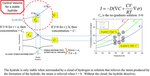
The upper left corner of Figure 7 shows a diagram of a control volume for a stable hydride at constant temperature. At the centre of the control volume is the hydride. The hydride forms from a cloud of atomic hydrogen in solution; hydrogen atoms in solution aggregate because of the partial molar volume of hydrogen that pushes out against the lattice producing mutually attractive local tensile regions for other hydrogen atoms. When the hydride forms the tensile stress gradient is increased because the metal hydride takes more volume than the metal from which it forms. The result is an elastic tensile stress distribution shown in the lower left corner of Figure 7. The distribution is truncated at the yield strength of the metal to avoid the singularity that would otherwise occur for a radial extent of zero, i.e., r=0  . The truncation defines a region around the hydride extending to r=a   as shown in Figure 7. In this region, the stress gradient is zero. In addition, there will be no concentration gradient in this region if the flux is zero according to the flux equation shown in the upper right corner of Figure 7, which is the case for constant temperature so that the Soret flux in Equation 1(1) $\mathrm{J}=-\mathit{D}\left(\mathrm{\nabla C}+\frac{\mathit{CV}}{\mathit{RT}}\mathrm{\nabla \sigma }+\frac{C{Q}^{\ast }}{\mathit{R}{T}^2}\mathrm{\nabla T}\right).$(1) is not included. This region where there are no gradients in concentration and stress is associated with the solvus concentration, C_o, defined by dynamic equilibrium between hydrogen in solution and hydrogen in hydride form.

Stable hydrides form in a control volume where the concentration in a small region adjacent to the hydride equals the solvus, and where the concentration equals C- at the extent of the control volume defined to be where the gradient of the stress because of hydride formation goes to zero. C- is a zero-flux solution to the equation shown in the upper right corner of Figure 7 obtained by equating the bracketed term to zero, integrating, and solving for concentration as described in [12]. There are two solutions, C+ and C- that differ in the sign of the exponential argument, these solutions exist if hydrides are present. The hydrostatic stress is written equal to the yield strength multiplied by a stress concentration factor, K.

(4) $\mathit{C}\text{-}(\mathit{T})=C_{\mathrm{o}}(\mathit{T})exp\left(\frac{-KV{\sigma }_y}{\mathit{RT}}\right),$(4)

where C_o is the solvus, and σ_y is the yield strength. The C- values shown in this paper were taken from figure 2 in [11] where they were used to explain the thermodynamics and kinetics of changing hydride X-ray diffraction peaks in Zircaloy-4 in terms of three zero-flux (i.e., J = 0) isothermal solutions to Equation 1(1) $\mathrm{J}=-\mathit{D}\left(\mathrm{\nabla C}+\frac{\mathit{CV}}{\mathit{RT}}\mathrm{\nabla \sigma }+\frac{C{Q}^{\ast }}{\mathit{R}{T}^2}\mathrm{\nabla T}\right).$(1) – these values for C- are estimates because the yield strengths for the materials analyzed in this paper were not reported in the original publications. The three zero-flux isothermal solutions are shown in the graph on the right of Figure 7. Inside the zero-flux curves J < 0, hydrogen moves towards the hydride and the hydride grows, while outside the curves J > 0, hydrogen moves away from the hydride and the hydride dissolves. The conditions for a stable hydride are shown by Points 1 and 2 on the graph for 570 K. Point 1 shows the concentration of hydrogen in solution in the region adjacent to the hydride equal to the solvus, i.e., for r < a, C(a) = C_o. Point 2 shows C(b) lies on the C- curve. Vertical lines connecting C_o to C- are indicative of stable hydrides. Thus, when the concentration of hydrogen in solution in the bulk matrix exceeds C-, stable hydrides can form: the region between the control volumes of stable hydrides will be at C-, which is the concentration that stabilizes the hydrides at the cores of the control volumes. In the figures of this paper, concentration-temperature slopes change when C- is exceeded indicative of hydride formation.

When stable hydrides are heated or cooled the concentrations C(a) and C(b) do not change at the same rate because the region adjacent to the hydride is thin compared with the much larger volume between hydrides which all share the same value of C-. In addition, C(a) is in dynamic equilibrium with the hydride so the concentration of hydrogen in solution for r<a, C(a), changes much faster than the concentration between control volumes. The result is that C(b) noticeably lags C(a) for practical temperature rises of about 1 to 20 K/min. In Figure 7, when the stable hydride associated with Points 1 and 2 at 570 K is heated to 580 K, Point 1 follows the solvus curve to Point 3. Point 2 goes to Point 4, its concentration does not immediately change with heating as does Point 1. Point 4 is in the J > 0 part of the graph so the hydride is unstable and dissolves and the concentration of hydrogen in solution in the bulk rises until it reaches Point 5 where the hydride is stable again. When cooling from 570 K to 560 K, Point 1 moves to Point 6 along the solvus curve, and Point 2 moves to Point 7. Point 7 is in the J < 0 part of the graph so hydrogen moves to the hydride and the concentration of hydrogen in solution in the bulk between control volumes falls from Point 7 to Point 8 where the hydride is stable. If instead of one specimen heated and cooled to discrete points, there were one specimen with initial hydrogen in solution of 84 wt.ppm (i.e., the horizontal line between Points 7 and 4) subjected to a positive temperature gradient, then you would see this horizontal line rotate counterclockwise about Point 2 to align with the C- curve between Points 8 and 5. The concentration gradient between Points 8 and 5 is positive in this illustrative example because Q* is zero. The concentrations after heating or cooling to discrete points between Points 8 and 5 will be the same as those for a single specimen subject to a temperature gradient. The reason in both cases is because there is nothing in the flux equation shown in the upper right corner of Figure 7 that allows movement of hydrogen to regions of different temperatures. To move hydrogen along the temperature gradient requires the Soret term in Equation 1(1) $\mathrm{J}=-\mathit{D}\left(\mathrm{\nabla C}+\frac{\mathit{CV}}{\mathit{RT}}\mathrm{\nabla \sigma }+\frac{C{Q}^{\ast }}{\mathit{R}{T}^2}\mathrm{\nabla T}\right).$(1) , and a non-zero Q*.

When Q* is positive and the temperature gradient is also positive a negative flux will result that moves hydrogen in the direction of the cold end of the specimen. In this case, for example at 580 K, there will be a competition for the hydrogen that comes from the dissolving hydrides that would otherwise raise the concentration of hydrogen in solution from Points 4 to 5 if Q* were zero, and the hydrogen moving to lower temperatures because of the positive Q* in the Soret term. The hydrogen would all move to the cold end except for the resulting negative concentration gradient that produces a Fick’s current that opposes the Soret current; hydrogen will cease moving when all opposing currents are equal so that J = 0. In this example, the initially horizontal line connecting Points 7 and 4 would rotate in the clockwise direction about Point 2 and stop when J = 0. Similar clockwise rotation is seen in the absence of hydrides: for the flux described by Equation 1(1) $\mathrm{J}=-\mathit{D}\left(\mathrm{\nabla C}+\frac{\mathit{CV}}{\mathit{RT}}\mathrm{\nabla \sigma }+\frac{C{Q}^{\ast }}{\mathit{R}{T}^2}\mathrm{\nabla T}\right).$(1) to be zero, a negative sign for the gradient for concentration is required if the temperature gradient and Q* are both positive. This clockwise rotation to produce a negative concentration-temperature slope is seen in all the plots shown in this paper; it is inferred from the durations the experiments quoted by the authors who made the measurements analyzed in this paper that sufficient time expired for the flux to go to zero.

The mobile solute phase is atomic hydrogen in solution. Hydrides that would otherwise be stable at high temperatures dissolve when the concentrations of hydrogen in solution at the periphery of their control volumes fall to values below C- because of the flow of hydrogen in solution away from the hot regions. At lower temperatures along the temperature gradient, concentrations are raised above C- by the flow of hydrogen in solution away from the hot regions into colder regions and stable hydrides can precipitate. So, hydrides will disappear from hot regions and appear in colder regions. It seems as if hydrides are diffusing from the hot end to the cold end because the process is limited by the diffusion of hydrogen in solution. The word ostensible (meaning apparent but not necessarily real) was coined by Maki and Sato [17] to describe ‘hydride diffusion,’ but the word ostensible suggests that the hydrides are not really diffusing, they just seem to be diffusing. Hydrides ostensibly move like pollen on the surface of a river entrained by an undercurrent of hydrogen in solution that moves downstream to regions where the temperature is lower [19]. Pollen experiences Brownian motion because of uneven numbers of collisions with water molecules at the periphery of the pollen providing transient impulsive forces that randomly change with time. In the same way, hydrides in dynamic equilibrium with hydrogen in solution will exhibit uneven transient growth and dissolution around their peripheries. These fluctuations in the extent of the peripheral boundaries of stable hydrides will display as Brownian motion – thus, regions where there are stable hydrides will fluctuate and move. Stable hydrides in a temperature gradient likewise move because of precipitation on the leading cold end, and dissolution on the trailing hot end of a hydride. The concentrations vary according to the flux equation, which is a diffusion equation, so technically hydrides are diffusing – by this definition, objects that obey the diffusion equation are said to be diffusing.¹ In the case of hydrides, individual atoms in the diffusing hydride will change, but it is expected that hydrides and hydrogen in solution should both obey the flux equation because the chemical potentials are connected for hydrogen for both cases because they are equal at J = 0, as mentioned in the Introduction. This expectation can be expressed equivalently as follows, to paraphrase the conclusion of Einstein’s Brownian motion paper: solute ‘hydrogen atoms in solid solution’ and suspended particles, such as hydrides, are identical in their behaviour differentiated solely by their dimensions [2].² Thus, the flux equation derived from the chemical potential of hydrogen in solution should work as well for hydrides. The reference to Einstein’s Brownian motion paper [2] is a reminder that there is nothing explicit in the flux equation that precludes using Equation 2(2) $Q^{\ast }=-\frac{R{T}^2}{\mathit{C}}\left(\frac{\mathit{dC}}{\mathit{dT}}+\frac{\mathit{CV}}{\mathit{RT}}\frac{\mathit{d\sigma }}{\mathit{dT}}\right),$(2) to calculate an apparent Q* for situations where hydrides are present – the maths are the same, only the slope changes as can be seen in Figure 6 for concentrations above C- where hydrides are predicted to occur. In another example, where the temperature was constant, the same effect of ostensible hydride diffusion was inferred to occur when an uneven initial distribution of hydrides evolves into a distribution of hydrides throughout the material that is indistinguishable at long times [20]; this being the definition of ultimate equilibrium when hydrides are present.

The flux of hydrogen is higher (i.e., by about five-times for these experiments) when hydrides are diffusing compared with simple diffusion of hydrogen in solution. The C+ and C- curves are only present when stable hydrides are present so the plots in Figure 7 are no longer applicable for concentrations below C-; hydrogen clouds still form, and intermittent hydrides will form but they will be unstable because the concentration of available hydrogen in the lattice is not enough to stabilize the hydrides (i.e., for the concentration to reach C-), so the intermittent hydrides dissolve then reform and dissolve and reform repeatedly. Perhaps, when hydrides are present, hydrogen in solution effectively carries more hydrogen in its wake because of the coupling with the hydrogen in the hydrides through the control volume stability constraint. Thus, hydrides appear to diffuse according to the flux Equation 1(1) $\mathrm{J}=-\mathit{D}\left(\mathrm{\nabla C}+\frac{\mathit{CV}}{\mathit{RT}}\mathrm{\nabla \sigma }+\frac{C{Q}^{\ast }}{\mathit{R}{T}^2}\mathrm{\nabla T}\right).$(1) but with a Q* that is five-times larger; the heat of transport and the associated force required to drag (or push) hydrides to lower temperature is about five-times greater than that needed to drag hydrogen in solution. More precisely, the heat of transport for moving hydrogen in solution is higher if hydrides are present than if they are not present.

An interesting observation seen in Figure 4 is that concentrations for specimens 4 and 5 appear to follow something akin to C-, but with higher values, at the hot end instead of continuing the straight line seen at lower temperatures into the region below C- where stable hydrides do not to exist. When approached from above, as in Figure 4 for specimens 4 and 5 at the hot ends of the specimens, the C- line is not crossed. The concentration of hydrogen at the hot ends for these specimens is at the minimum value, i.e., C-, that would sustain stable hydrides, and the concentration-temperature slope follows the C- curve like it did between Points 8 and 5 in Figure 7 in the illustrative example when Q* was zero as described previously; apparently following the higher entropy production path affiliated with the Soret current is preferred over the path associated with the drift current. But, when C- is approached from below as in Figure 6, the C- line is not an impediment, perhaps to facilitate higher entropy production. More experiments like those in [17] starting with hydrides everywhere should be done with total concentrations close to C-, and for longer times to ensure that J = 0 is indeed reached, so that this possible reticence to cross the C- curve from above can be better quantified.

5. Applications

The heat of transport is used within the flux equation to calculate hydrogen profiles that result from temperature gradients in reactor core components made of zirconium alloys. One example is found in Zircaloy fuel cladding in Light Water Reactors. The Hydride Nucleation-Growth-Dissolution (HNGD) model is being advanced to predict concentrations of hydrogen in cladding in the nuclear fuel performance code Bison developed at the Idaho National Laboratory [4]. The default model uses Equation 1(1) $\mathrm{J}=-\mathit{D}\left(\mathrm{\nabla C}+\frac{\mathit{CV}}{\mathit{RT}}\mathrm{\nabla \sigma }+\frac{C{Q}^{\ast }}{\mathit{R}{T}^2}\mathrm{\nabla T}\right).$(1) but without the drift term, so the flux includes just the Fick’s current and the Soret current. Figure 5 shows how ‘the [HNDG] model fails to predict the hydride profile on the left of the sample’ for positions less that 0.45 cm [21]. The data in the figure were obtained from measurements of hydrogen concentrations along a 4-cm sample after 150 days subject to the asymmetric temperature profile shown by the curve. The HNDG default predictions are made with the Q* determined in the absence of hydrides, so Q* is 25 kJ/mol. But hydrides will be present when concentrations exceed C-: the C- concentration is 46 wt.ppm at 546 K taken from figure 2 in [11]; these values are connected by the vertical dashed line in Figure 5. Thus, the HNDG fails to predict the hydrogen concentration profile on the left of the sample in Figure 5 because the Q* used in the model is not appropriate when hydrides are present – this explanation is a conclusion of the current paper.

A different explanation for the discrepancy between the HNDG predictions and the observations was proposed in [21]. This explanation is based on an interpretation of hydrogen and hydrides in zirconium that invokes two terminal solid solubility (solvi) relationships, even thought Gibbs’ Phase Rule explicitly forbids two solvi; there can only be one solvus for a two-component two-phase system for constant hydrostatic pressure between control volumes [1,12]. Regardless two solvi are defined: one for cooling leading to precipitation called TSSP, and one for heating leading to dissolution called TSSD [12]. TSSP concentrations are above TSSD concentrations, the difference is called an apparent hysteresis [1,22]. To explain the discrepancy, the TSSP and TSSD relationships were modified. TSSP was identified as a supersolubility with a time dependency for the hysteresis such that over a few hours TSSP became equal to TSSD. In addition, TSSD was identified as the solubility and various new parameters were added to raise it to an effective value that depends on hydride content. The parameters used to tweak the TSS relationships are seemingly not determinable by regression of the model to observations, and they do not seem to be calculable a priori. In essence, the solubility limits are ‘improved’ by introducing ~ 6 new parameters in polynomial equations, and a decay equation (surprisingly without a temperature dependence) to account for the discrepancy of the HNDG model when hydrides are present. These adjustments are required because of the assumption that TSSP represents a supersaturated state and TSSD is the thermodynamic solubility, but there are other interpretations [23].

None of these adjustments are required if instead the thermodynamic solubility limit is associated with the onset of precipitation, and if instead, the point where the slopes change equals C-. The region between stable hydrides will also be at C-, as described in [1] and the previous discussion of Figure 7. Presumably, the adjustments that modify the HNDG model are able to raise and lower TSSD and TSSP to match C- at the appropriate times. By contrast, C- is predicted from independent measurements of yield strength, partial molar volume of hydrogen in solution, diffusivity of hydrogen in solution, and a single solvus in accord with Gibbs’ Phase Rule, and a stress concentration factor for plane stress conditions for hydrides inferred from experiments and calculated from fracture mechanics, as described in [12] – there is no wiggle room in the calculation of C-, there are no additional parameters needed as shown in Equation 4(4) $\mathit{C}\text{-}(\mathit{T})=C_{\mathrm{o}}(\mathit{T})exp\left(\frac{-KV{\sigma }_y}{\mathit{RT}}\right),$(4) .

Another example of using the flux equation to calculate hydrogen profiles is the rolled joint (RJ) in CANDU fuel channels where the Zr-2.5Nb pressure tube is rolled into an end fitting made of 403 Stainless Steel. In these examples, hydrides are invariably present so the Q* is not 25 kJ/mol. Instead, for most reactor applications of interest where hydrides are present, Q* = (116 ± 17) kJ/mol. The implication of using the Q* measured with hydrides present is that the final J = 0 state will be different. As an example, the concentration of hydrogen isotopes can exceed C- in the RJ region of pressure tubes so hydrides are present during operation. It has been observed that there is a circumferential distribution of hydrogen in the horizontal tubes, with high concentrations at the 12 o’clock position (see figure A1 in [24]). At the outlet RJ where the coolant exits the core, this circumferential distribution has been attributed to a temperature gradient with the top of the tube being 20 °C lower than the bottom of the tube. This temperature variation is attributed to flow bypass: at about 5 m from the inlet of the 6-m pressure tube, the pressure tube expands radially late in life (about 3% after 13 effective full-power years) because of the combined effects of irradiation creep and growth, pressure, and temperature. This expansion allows coolant to bypass the fuel bundle, flowing over the bundle and not being heated to the extent it would be if it flowed through the bundle. The top-to-bottom temperature difference of 20 °C is calculated from the observed circumferential hydrogen concentration gradient and the Q* determined in the absence of hydrides. With the appropriate Q* in the presence of hydrides, the temperature gradient will be five times smaller, or 4 °C. This smaller temperature gradient is in accord with the predictions of deuterium-concentration profiles emanating from the RJ into the reactor core [25]. A top-to-bottom temperature difference of 20 °C in the tube at the RJ based on flow bypass at 5 m is difficult to defend when the tube remains at its original diameter after 5 m, so that the coolant will be constrained to pass through two more bundles where it will be mixed by turbulent flow before it reaches the RJ. A difference of 20 °C is substantial compared with the temperature rise along the length of the pressure tube of about 60 °C. Using the new value of Q* in the presence of hydrides reduces this temperature gradient to a believable value of 4 °C [26].

The discussion so far has been focused on the final J = 0 distribution that is attained regardless of the initial conditions of local concentrations. If the concentrations are high enough (i.e., always above C-), or low enough (i.e., always below C-), then the concentrations evolve locally with rates limited by the terminal velocities in the coldest regions: the concentration temperature profile rotates about a steady-state point stopping when there is no net flux (i.e., when the concentration gradient in Equation 1(1) $\mathrm{J}=-\mathit{D}\left(\mathrm{\nabla C}+\frac{\mathit{CV}}{\mathit{RT}}\mathrm{\nabla \sigma }+\frac{C{Q}^{\ast }}{\mathit{R}{T}^2}\mathrm{\nabla T}\right).$(1) , plus the drift term, cancel the Soret current so that J = 0). If the concentrations cross C-, then there will be two concentration-temperature profiles, one for the region where there are two solid phases (i.e., hydrides and zirconium with concentrations of hydrogen above C-) and another for the single solid-phase region (i.e., just zirconium, no hydrides, the region below C-). The transient profiles will depend on the initial concentration profile. For example, consider a uniform initial profile that spans both the two-phase and single-phase regions. The horizontal lines of these profiles will rotate with time until the final J = 0 conditions are met. The line for the single-phase region will rotate and fall as hydrogen moves from the region with concentrations less that C- to the colder region where concentrations are above C- and hydrides can form – the line will also lengthen on the cold side so that it remains in contact with the C- curve. Simultaneously, hydrides in the two-phase region that are destabilized because of the rotation, falling, and lengthening of the single-phase line, dissolve putting hydrogen into solution that moves to the cold end of the rotating, falling, and lengthening single-phase line where it precipitates as a front of hydrides. Eventually, the rotation is sufficient for no net flux to happen, and no more changes occur in the single-phase region. In contrast, the line for the two-phase region rotates, rises, and shortens. The hydride front redistributes in the two-phase region to the final concentration profile there. Examples of the concentration profile showing the hydride front are shown in figures 4 and 5 in [5]; the horizontal axes in these figures can be directly related to temperature using the reported linear temperature range. An example of crossing the C- line from above might be seen in specimens 4 and 5 shown in Figure 4 as discussed earlier. In these specimens the rotation of the two-phase line seems to be frustrated by the lower Q* of the single-phase region. For practical applications, these transients are not important if the component is in reactor for enough time for the final zero-flux state to happen, years would certainly be enough time, and the ingress rate of hydrogen isotopes into the metal during operation is slow compared with how fast the final state is reached.

Finally, different values for Q* depending on whether stable hydrides are present suggest that different values for the partial molar volume might likewise occur. It would be interesting to see the results of a stress-gradient experiment with and without stable hydrides present [27]. By analogy with Equation 2(2) $Q^{\ast }=-\frac{R{T}^2}{\mathit{C}}\left(\frac{\mathit{dC}}{\mathit{dT}}+\frac{\mathit{CV}}{\mathit{RT}}\frac{\mathit{d\sigma }}{\mathit{dT}}\right),$(2) , for J = 0, the analysis equation would be $\mathit{V}=(\mathit{RT}/\mathit{C})\mathrm{\nabla C}/\mathrm{\nabla }\mathit{\sigma }.$

6. Conclusions

This current analysis suggests that the value for the heat of transport used in Bison does not need to change if stable hydrides are absent, in which case Q* = (25 ± 3) kJ/mol. But, if stable hydrides are present, then Q* = (116 ± 17) kJ/mol. For completeness, the drift stress term could be added to the flux equation used in Bison.

Disclosure statement

No potential conflict of interest was reported by the author(s).

Notes

1. Although some people might prefer to identify hydrogen in solution as the diffusing species and say that hydrides ostensibly diffuse, or that hydrides dissolve in one location and reprecipitate in another; the important point is that the flux equation represents the observed concentrations in a temperature gradient, which is what is required to make assessments of in-reactor components.

2. ‘Nach dieser Theorie unterscheidet sich eingelöstes Molekül von einem suspendierten Körper lediglich durch die Gröβe,’ [p. 550]; (According to this theory, a dissolved molecule is differentiated from a suspended body solely by its dimensions.), ‘… Moleküle und suspendierte Körper von gleicher Anzahl sich in bezug auf osmotischen Druck bei großer Verdünnung vollkommen gleich verhalten.’ [p. 553]. (Molecules and suspended bodies of equal number behave perfectly alike with respect to osmotic pressure at great dilution.)

References

- McRae GA, Coleman CE. Rival interpretations of hydride precipitation-dissolution hysteresis in zirconium: rebuttal to critical comments to the letter to the editor of G.A. McRae and C.E. J Nucl Mater. 2022;568(568):153889. doi: 10.1016/j.jnucmat.2022.153889
- Einstein A. Über die von der molekularkinetischen Theorie der Wärme geforderte Bewegung von in ruhenden Flüssigkeiten suspendierten Teilchen. Ann Phys. 1905;322(8):549–560. doi: 10.1002/andp.19053220806
- Eastman ED. Theory of the Soret effect. J Am Chem Soc. 1926;48(6):1482–1493. doi:10.1021/ja01417a004
- Kang S, Huang P-H, Petrov V, et al. Determination of the hydrogen heat of transport in Zircaloy-4. J Nucl Mater. 2023;573:154122. doi: 10.1016/j.jnucmat.2022.154122
- Sawatzky A. Hydrogen in Zircaloy-2: its distribution and heat of transport. J Nucl Mater. 1960;2(4):321–328. doi: 10.1016/0022-3115(60)90004-0
- Caskey GR, Cole GR, Holmes WG. Failure of UO2 fuel tubes by internal hydriding of Zircaloy-2 sheaths, Proc. Symp. On powder packed uranium dioxide fuel elements, CEND-153 II. Paper IV-E-1. Windsor, CT: USA–Euratom, Combustion Engineering; 1961.
- Perryman ECW. Pickering pressure tube cracking experience. Nucl Energy. 1977;17:95–105.
- Field GJ, Dunn JT, Cheadle BA. Analysis of the pressure tube failure at Pickering NGS “A”Unit 2 nuclear systems department. Can Metall Q. 1985;24(3):181–188. doi: 10.1179/cmq.1985.24.3.181
- Edsinger K, Davies JH, Adamson RB. Degraded fuel cladding fractography and fracture behavior, Zirconium in the Nuclear Industry: Twelfth International Symposium, Proc. ASTM STP 1354, Toronto, 1998; Sabol GP GD Moan, editors. West Conshohocken, PA: ASTM International; 2000. p. 316–339
- Kubo T, Kobayashi Y, Uchikoshi H. Measurement of delayed hydride cracking propagation rate in the radial direction of Zircaloy-2 cladding tubes. J Nucl Mater. 2012;427(1–3):18–29. doi: 10.1016/j.jnucmat.2012.04.012
- McRae GA, Coleman CE. Zirconium hydride precipitation in Zircaloy-4 during rapid cooling followed by isothermal interludes observed with synchrotron X-ray diffraction. J Nucl Mater. 2022;565:153729. doi: 10.1016/j.jnucmat.2022.153729
- McRae GA, Coleman CE. Precipitates in metals that dissolve on cooling and form on heating: an example with hydrogen in alpha-zirconium. J Nucl Mater. 2018;499:622–640. doi: 10.1016/j.jnucmat.2017.09.017
- Kim JH, Lee MH, Choi BK et al. Deformation behavior of Zircaloy-4 cladding under cyclic pressurization. J Nuc Sci Tec. 2007;44(10):1275–1280. doi: 10.1080/18811248.2007.9711371
- Coleman CE, Adamson RB, Cox B, McRae GA. et al. Chapter 9, Ductility and Fracture, The Metallurgy of Zirconium. Vienna: IAEA; 2023.
- Kammenzind B, Franklin D, Peters H et al. Hydrogen pickup and re-distribution in alpha-annealed Zircaloy-4. ASTM STP. 1996;1295:338–370. doi: 10.1520/STP16180S
- Merlino JT. Experiments in hydrogen distribution in thermal gradients calculated using bison, M.Eng paper in nuclear engineering. The Pennsylvania State University. 2019.
- Maki H, Sato M. Thermal diffusion of hydrogen in Zircaloy-2 containing hydrogen beyond terminal solid solubility. J Nucl Sci Tec. 1975;12(10):637–649. doi: 10.1080/18811248.1975.9733165
- Shewmon PG. Diffusion in solids. Toronto: McGraw-Hill. 1963; p. 190–191.
- Brown R. XXVII. A brief account of microscopical observations made in the months of June, July and August 1827, on the particles contained in the pollen of plants; and on the general existence of active molecules in organic and inorganic bodies. Philos Mag. 1828;4(21):161–173. doi: 10.1080/14786442808674769
- McRae GA, Coleman CE, Nordin HM. Predictions of ingress of hydrogen isotopes for zirconium alloys should not be based on solubility limits. J Nucl Mater. 2022;566:153755. doi: 10.1016/j.jnucmat.2022.153755
- Passelaigue F, Simon P-C, Motta AT. Predicting the hydride rim by improving the solubility limits in the hydride nucleation-growth-dissolution (HNGD) model. J Nucl Mater. 2022;558:153363. doi: 10.1016/J.JNUCMAT.2021.153363
- McRae GA, Coleman CE. The Zr α-phase/(α-phase + hydride) transformation should obey the phase rule. J Nucl Mater. 2021;556:153169. doi: 10.1016/j.jnucmat.2021.153169
- McRae GA, Coleman CE. Response to Puls’ critique of the McRae-Coleman interpretation of the Zr-H solubility limit. J Nucl Mater. 2023;581:154423. doi: 10.1016/j.jnucmat.2023.154423
- Hydrogen Equivalent Concentration in Pressure Tubes for Nuclear Power Plants, Canadian Nuclear Safety Commission, 2021 Sept 3. Report No: CMD 21-M37.1.
- McRae GA, Coleman CE. Deuterium concentration profiles at the rolled joints of CANDU fuel channels. J Nucl Mater. 2023;573:154128. doi: 10.1016/j.jnucmat.2022.154128
- Greening F. CNSC staff update on elevated hydrogen equivalent concentration discovery events in the pressure tubes of reactors in extended operation, addendum 2. Canadian Nuclear Safety Commission. Nov. 2022;3:171–227.
- Eadie RL, Tashiro K, Harrington D, et al. The determination of the partial molar volume of hydrogen in zirconium in a simple stress gradient using comparative microcalorimetry. Scr Metall Mater. 1991;26(2):231–236. doi: 10.1016/0956-716X(92)90178-H