Predictive Control Charts (PCC): A Bayesian approach in online monitoring of short runs

Abstract

Performing online monitoring for short horizon data is a challenging, though cost effective benefit. Self-starting methods attempt to address this issue adopting a hybrid scheme that executes calibration and monitoring simultaneously. In this work, we propose a Bayesian alternative that will utilize prior information and possible historical data (via power priors), offering a head-start in online monitoring, putting emphasis on outlier detection. For cases of complete prior ignorance, the objective Bayesian version will be provided. Charting will be based on the predictive distribution and the methodological framework will be derived in a general way, to facilitate discrete and continuous data from any distribution that belongs to the regular exponential family (with Normal, Poisson and Binomial being the most representative). Being in the Bayesian arena, we will be able to not only perform process monitoring, but also draw online inference regarding the unknown process parameter(s). An extended simulation study will evaluate the proposed methodology against frequentist based competitors and it will cover topics regarding prior sensitivity and model misspecification robustness. A continuous and a discrete real data set will illustrate its use in practice. Technical details, algorithms, guidelines on prior elicitation and R-codes are provided in appendices and supplementary material. Short production runs and online phase I monitoring are among the best candidates to benefit from the developed methodology.

Keywords:

• Online phase I monitoring
• outlier detection
• regular exponential family
• self-starting
• statistical process control and monitoring

1. Introduction

In Statistical Process Control/Monitoring (SPC/M) of either discrete or continuous univariate data, various frequentist based parametric methods have been developed, with the Shewhart type control charts, CUSUM and EWMA being the most dominant representatives. All these methods utilize the information coming from the likelihood to draw control limits, aiming to detect when the process moves from the in control (IC) state, where it runs under random natural variation, to the out of control (OOC) state, where exogenous to the process variation is present (Deming 1986). Typically, although not necessarily, in SPC/M the OOC state reflects either transient shifts (of large size) or persistent shifts (of medium/small size) that occurs in the unknown parameter(s), with detection being of main interest. The Shewhart type charts are employed to detect large transient shifts, while CUSUM and EWMA are more effective in identifying small persistent shifts. All these methods require knowledge of the IC process parameter(s), a matter handled in practice by the employment of an offline calibration (phase I) period, prior to the online monitoring of the process (phase II). Phase I estimation requires a relatively long sequence of independent and identically distributed (iid) data points from the IC distribution. Once the phase I data collection completes, the unknown parameter(s) estimation and the chart construction begins. Initially, all the phase I data are analyzed retrospectively and in case of alarms, observations might be removed and control limits might be revised. Next, once the control chart is finalized, online monitoring starts for phase II data, where we test whether the phase II data conform to the control limits established during phase I. It is well established and documented that phase I plays a crucial role, as undetected phase I issues (like masked outlying observations), will contaminate the parameter(s) estimates and the resulting control limits, jeopardizing the phase II performance. Jensen et al. (2006) provided a nice review on the effect of estimation error, while Zhang et al. (2013), Zhang, Megahed, and Woodall (2014), and Lee et al. (2013) showed that an excessively large amount of IC phase I data is required for a similar performance as if the IC parameter(s) were known. More recently, Dasdemir et al. (2016) evaluated the phase I analysis and Atalay et al. (2020) provided guidelines for automating phase I considering the phase II performance.

The phase I/II setup is known to have certain limitations. For example, it is not applicable in short runs, as the data size is too small to allow a phase I procedure (an industrial example of this type is presented in Section 6). Furthermore, it cannot be employed when the process under study requires online and not retrospective monitoring during phase I, as it happens in health type variables (such as the medical laboratory monitoring case that we present in Section 6). Jones-Farmer et al. (2014), presented a detailed overview of methods that could be employed for short runs, with the self-starting methods probably being the ones most often applied in practice. As the name declares, such methods do not require a phase I/II separation and they are able to be up and running soon after the process starts. The idea behind the frequentist-based self-starting methods is to perform calibration and testing simultaneously. Focusing in outlier detection, Quesenberry (1991a, 1991b, 1991c) introduced the self-starting versions of standard Shewhart type control charts, known as Q-charts. On the other hand, when the aim is in detecting small persistent shifts, self-starting CUSUMs and EWMA were suggested by Hawkins and Olwell (1998) and Qiu (2014) respectively. In more recent studies, a bootstrap based self-starting EWMA monitoring scheme for Poisson count data was proposed by Shen et al. (2016). Within the frequentist-based approach, non-parametric methods, like the recursive segmentation and permutation (RS/P) (Capizzi and Masarotto 2013) or the sequential non-parametric tests (Madrid Padilla et al. 2019), have been also suggested to handle univariate data. Non-parametric methods are capable to identify small persistent shifts, while for transient shifts they require subgrouped data and/or a relative long sequence of observations. From all the aforementioned start-up frequentist based methods, only the Q-charts are built to identify transient shifts of large size (outliers) in short individual data, while the rest are more powerful in detecting small persistent shifts, like step changes.

The Bayesian approach to SPC/M is rather restricted. Menzefricke (2002) suggested the use of the predictive distribution for constructing a control chart, which was next compared to Shewhart type charts for Normal and Binomial data. Kumar and Chakraborti (2017) along with Ali (2020), presented Bayesian versions of Shewhart type charts for time between events monitoring, while Kadoishi and Kawamura (2020) suggested a hierarchical Bayesian modeling when we have data from a time series model IMA(1,1). Apley (2012), introduced the posterior distribution plots that aim to monitor the process mean during phase II. Regarding phase I analysis, Woodward and Naylor (1993) used Bayesian modeling to handle short runs of Normal data, while Tsiamyrtzis and Hawkins (2005, 2010, 2019) provided a Bayesian change point approach using a mixture of distributions in modeling Normal or Poisson phase I data.

In this work, we propose a general Bayesian method that intends to provide efficient online monitoring of a process for short runs, without the requirement of a phase I/II separation, focusing on outlier detection. As a self-starting Bayesian method, it will utilize the available prior information (or adopt an objective Bayesian approach in scenarios of complete prior ignorance), providing a sequentially updated scheme that will be based on the predictive distribution. Precisely, we will introduce the Predictive Control Chart (PCC), which will be able to perform online monitoring, directly after the first observable becomes available. PCC will be formed as a sequentially updated region, against which every incoming data will be plotted, providing either conformance of the data with what has been foreseen from the predictive distribution or nonconformance, raising an alarm. PCC will be introduced in a general form, allowing to handle data of any (discrete or continuous) distribution, as long as this distribution is a member of the regular exponential family. The vast majority of the distributions used in SPC/M, with Normal, Poisson and Binomial being the most indicative cases, are members of the regular exponential family. The core idea of PCC, i.e., the sequential testing on the updated predictive distribution, can be extended in other distributions. However, the regular exponential family guarantees a general closed-form predictive distribution.

In Section 2, we provide the PCC derivation, along with the necessary formulas for several discrete and continuous univariate distributions that belong to the regular exponential family. We also present the PCC options that allow the use of possibly available historical data, via a power prior mechanism, and the possibility of employing a Fast Initial Response (FIR) PCC, which enhances its performance during the early stages of the process. Next, in Section 3 we provide the PCC based decision making, where apart from being able to control and monitor the process, we are capable of deriving online inference (in terms of point/interval estimates or hypothesis testing) for the unknown parameter(s) and perform forecasting. In Section 4, we present an extended simulation study, where we evaluate the PCC performance against its frequentist-based alternative, i.e., Q-chart (Quesenberry 1991a, 1991b, 1991c) and we additionally examine issues regarding prior sensitivity. The PCC robustness when we have dependent data or distribution misspecifications is examined in Section 5. The PCC application to real data follows in Section 6, where a continuous (Normal) and a discrete (Poisson) real-data case from a medical lab and an industrial setting respectively, are being explored. Finally, Section 7 provides the concluding remarks. Technical details, algorithms and guidelines regarding choices of prior distributions are provided as appendices along with R-codes as online supplementary material, and via GitHub at https://github.com/BayesianSPCM/BSPCM.

2. Predictive control chart

Being in the Bayesian framework, our goal is to utilize the available prior information and provide a control chart with enhanced performance compared to existing self-starting frequentist-based methods. The proposed Predictive Control Chart (PCC) will be formed by the predictive distribution and it will provide a sequentially updated region against which every new observable will be plotted. Observations falling outside the predictive region will ring an alarm triggering further investigation and potentially some form of corrective action.

Initially, we need to derive the predictive distribution (Geisser 1993), which depends on the likelihood of the observed univariate data. From a process under study, we sequentially obtain the data $\mathit{X}=(x_1,\dots ,x_n),$ which we consider to be a random sample from the distribution $X_j|\mathit{\theta },$ where $X_j,j=1,\dots ,n,$ is univariate, while the unknown parameter $\mathit{\theta }$ can be either univariate or multivariate, e.g., $X_j|\theta \sim \mathit{Bin}(N_j,\theta ),X_j|\theta \sim P(\theta ),X_j|\mathit{\theta }\sim N({\theta }_1,{\theta }_2^2)$ etc. Our main interest is in detecting in an online fashion and without employing a phase I exercise, the presence of large transient shifts on the unknown parameter(s) $\mathit{\theta }.$ We assume that the likelihood, is a member of the univariate k-parameter regular exponential family (denoted from this point on as k-PREF), and by following Bernardo and Smith (2000), it can be written as: (1) $$f(\mathit{X}|\mathit{\theta })=\left[\prod _{j=1}^{n}g(x_j)\right]{[c(\mathit{\theta })]}^n\hspace{0.17em}\text{exp}\hspace{0.17em}\left\{\sum _{i=1}^k{\eta }_i(\mathit{\theta })\sum _{j=1}^n{h}_i(x_j)\right\},$$(1) where $g(x_j)\ge 0,h_1(x_j),\dots ,h_k(x_j)$ are real-valued functions of the univariate observation x_j that do not depend on $\mathit{\theta },$ while $c(\mathit{\theta })\ge 0$ and ${\eta }_1(\mathit{\theta }),\dots ,{\eta }_k(\mathit{\theta })$ are real-valued functions of the unknown parameter(s) $\mathit{\theta }$ that cannot depend on X. PCC will be developed for any likelihood that belongs to the k-PREF, providing a general platform where binary (Binomial), count (Poisson, Negative Binomial) or various continuous (Normal, Gamma, Lognormal etc.) univariate data can be analyzed using the same methodology.

The prior distribution is of key importance in the Bayesian approach. Since in practice, historical data (of the same or a similar process, not to be confused with phase I data) are typically available, we recommend the use of power priors (Ibrahim and Chen 2000), which offer a framework to incorporate past data (when available) in the mechanism of forming the prior distribution. The power prior is derived by: (2) $$\pi \left(\mathit{\theta }|\mathit{Y},{\alpha }_0,\mathit{\tau }\right)\propto f{\left(\mathit{Y}|\mathit{\theta }\right)}^{{\alpha }_0}{\pi }_0\left(\mathit{\theta }|\mathit{\tau }\right),$$(2) where $\mathit{Y}=(y_1,\dots ,y_{n_0})$ refers to a vector of historical univariate data (under the same distribution law $f(·|\mathit{\theta })$ that the current data obey), $0\le {\alpha }_0\le 1$ is a scalar parameter, ${\pi }_0(\mathit{\theta }|\mathit{\tau })$ is the initial prior for the unknown parameter(s) and $\mathit{\tau }$ is the vector of the initial prior hyperparameters. The (fixed) parameter, α₀, controls the power prior’s tail heaviness and consequently the influence of the historical data on the posterior distribution. Essentially, α₀ represents the probability of the historical data being compatible with the current observations and at the extremes ${\alpha }_0=0$ or 1, the historical data will be ignored or taken fully into account (just as the current data) respectively. A typical value for α₀ is $1/n_0,$ which conveys the weight of a single observation to the prior information. In general, α₀ should be determined by the relevance of past with current data and how likely is the past data to provide reliable estimates for the unknown parameters (depending on the size n₀). For relevant historical data but with small (large) n₀ it is recommended to use ${\alpha }_0<1/n_0({\alpha }_0>1/n_0).$ It should be noted that the power priors are robust in conflicts of historical and current data, as they use only the sufficient statistic of the past data.

Generalizing the power prior concept, we could either assume α₀ is unknown (modeled by a prior distribution) or we could allow the use of multiple historical data: if Y and Z are historical data from different sources weighted by α₀ and β₀ respectively, then the power prior is proportional to: (3) $$\pi \left(\mathit{\theta }|\mathit{Y},\mathit{Z},{\alpha }_0,{\beta }_0,\mathit{\tau }\right)\propto f{\left(\mathit{Y}|\mathit{\theta }\right)}^{{\alpha }_0}f{\left(\mathit{Z}|\mathit{\theta }\right)}^{{\beta }_0}{\pi }_0\left(\mathit{\theta }|\mathit{\tau }\right).$$(3)

It is worth mentioning that, Ibrahim, Chen, and Sinha (2003), proved that the power prior is 100% efficient in the sense that the ratio of the output to input information is equal to one, with respect to Zellner’s information rule (see Zellner 1988).

In a subjective Bayesian manner, ${\pi }_0(·)$ should reflect all available information regarding the unknown parameter(s) before the data become available and its form can be derived from prior knowledge, expert’s opinion etc. From an objective Bayesian point of view and under the scenarios of lacking any prior knowledge, one can adopt a weakly informative or even non-informative initial prior, such as flat (uniform) prior, Jeffreys (1961) or reference (Bernardo 1979; Berger, Bernardo, and Sun 2009) prior (see also the discussion regarding prior elicitation in Appendix E).

To preserve closed form solutions for all scenarios, when implementing PCC, we will adopt a conjugate prior for ${\pi }_0(\mathit{\theta }|\mathit{\tau }),$ which always exists for any likelihood that is a member of the k-PREF (Bernardo and Smith 2000) and its form is given by: (4) $${\pi }_0\left(\mathit{\theta }|\mathit{\tau }\right)={\left[K(\mathit{\tau })\right]}^{-1}{[c(\mathit{\theta })]}^{{\tau }_0}\hspace{0.17em}\text{exp}\hspace{0.17em}\left\{\sum _{i=1}^k{\eta }_i(\mathit{\theta }){\tau }_i\right\},$$(4) where $\mathit{\theta }\in \mathbf{\Theta }$ (parameter space) and $\mathit{\tau }=({\tau }_0,{\tau }_1,\dots ,{\tau }_k)$ is the $(k+1)$-dimensional vector of the initial prior hyperparameters, such that: (5) $$K(\mathbf{\tau })=\underset{\mathbf{\Theta }}{\int }{[c(\mathbf{\theta })]}^{{\tau }_0}\hspace{0.17em}\text{exp}\hspace{0.17em}\left\{\sum _{i=1}^k{\eta }_i(\mathbf{\theta }){\tau }_i\right\}d\mathbf{\theta }<\infty .$$(5)

The conjugate prior, ${\pi }_0(\mathit{\theta }|\mathit{\tau }),$ is also a member of the exponential family. The choice of the hyperparameters $\mathit{\tau }$ will reflect the prior knowledge, ranging from highly informative to vague and even non-informative choices. Non-conjugate choices of the initial prior are allowed, at the cost of not having PCC in closed form but evaluated numerically. A conjugate ${\pi }_0(\mathit{\theta }|\mathit{\tau })$ will lead to a conjugate power prior of the form (see Appendix A): (6) $$\pi \left(\mathit{\theta }|\mathit{Y},{\alpha }_0,\mathit{\tau }\right)\propto {\pi }_0\left(\mathit{\theta }|\mathit{\tau }+{\alpha }_0{\mathit{t}}_{n_0}(\mathit{Y})\right),$$(6) where ${\mathit{t}}_{n_0}(\mathit{Y})=(n_0,{\sum }_{l=1}^{n_0}{h}_1(y_l),\dots ,{\sum }_{l=1}^{n_0}{h}_k(y_l))$ is a $(k+1)$-dimensional vector, with $\mathit{Y}=(y_1,\dots ,y_{n_0})$ referring to the vector of historical univariate data. Theorem 1 provides, in closed form, the posterior and predictive distributions of any likelihood that belongs to the k-PREF (proof is given in Appendix A):

Theorem 1.

For any likelihood belonging to the k-PREF (1) and an initial conjugate prior (4) via a power prior (6) mechanism we have:

(i)The posterior distribution of the unknown parameter(s) $\mathit{\theta }$: (7) $$p\left(\mathit{\theta }|\mathit{X},\mathit{Y},{\alpha }_0,\mathit{\tau }\right)={\pi }_0\left(\mathit{\theta }|\mathit{\tau }+{\alpha }_0{\mathit{t}}_{n_0}(\mathit{Y})+{\mathit{t}}_n(\mathit{X})\right),$$(7) where ${\mathit{t}}_n(\mathit{X})=(n,{\sum }_{j=1}^n{h}_1(x_j),\dots ,{\sum }_{j=1}^n{h}_k(x_j))$ is a $(k+1)$-dimensional vector, with $\mathit{X}=(x_1,\dots ,x_n)$ being the observed univariate data.

(ii)The predictive distribution of the single future univariate observable $X_{n+1}$: (8) $$f\left(X_{n+1}|\mathit{X},\mathit{Y},{\alpha }_0,\mathit{\tau }\right)=\frac{K\left(\mathit{\tau }+{\alpha }_0{\mathit{t}}_{n_0}(\mathit{Y})+{\mathit{t}}_n(\mathit{X})+{\mathit{t}}_1(X_{n+1})\right)}{K\left(\mathit{\tau }+{\alpha }_0{\mathit{t}}_{n_0}(\mathit{Y})+{\mathit{t}}_n(\mathit{X})\right)}g(X_{n+1}),$$(8) where ${\mathit{t}}_1(X_{n+1})=(1,h_1(X_{n+1}),\dots ,h_k(X_{n+1}))$ is a $(k+1)$-dimensional vector, function of the future observable $X_{n+1}.$

PCC construction will be based on the predictive distribution and it can start as soon as n = 2 (except when we have Normal likelihood with both parameters unknown, ${\alpha }_0=0$ and we use the reference prior, where PCC starts at n = 3). The exact form of the predictive distribution (under conjugate prior), for various likelihood choices (either discrete or continuous data), used commonly in SPC/M, can be found in Table 1. To unify notation in the table, we denote by $\mathit{D}=(\mathit{Y},\mathit{X})=(y_1,\dots ,y_{n_0},x_1,\dots ,x_n)$ the vector of historical and current univariate data, $\mathit{w}=({\alpha }_0,\dots ,{\alpha }_0,1,\dots ,1)$ the vector of weights corresponding to each element d_j in D and finally we call $N_D=n_0+n$ the length of the data vector D.

Table 1. The predictive distribution using an initial conjugate prior in a power prior mechanism for some of the distributions typically used in SPC/M, which also belong to the k-PREF. $\mathit{D}=(\mathit{Y},\mathit{X})=(y_1,\dots ,y_{n_0},x_1,\dots ,x_n)$ is the vector of historical and current univariate data, $\mathit{w}=({\alpha }_0,\dots ,{\alpha }_0,1,\dots ,1)$ are the weights corresponding to each element d_j of D and $N_D=n_0+n.$

Distribution	Likelihood: $f(\mathit{x}|\mathit{\theta })$	Initial Prior: ${\pi }_0(\mathit{\theta }|\mathit{\tau })$	Predictive: $f(x_{n+1}|\mathit{D},\mathit{w},\mathit{\tau })$
Poisson (si=rate)	$X_i|\theta \sim$P$(\theta ·s_i)$	$\theta \sim$ G(c, d)	$f(x_{n+1}|\mathit{D},\mathit{w},\mathit{\tau },s_1,\dots ,s_n,s_{n+1})=$NBin$\left(c+{\sum }_{j=1}^{N_D}{w}_j{d}_j,\frac{s_{n+1}}{d+{\sum }_{j=1}^{N_D}{w}_j{s}_j+s_{n+1}}\right)$
Binomial (Ni=trials)	$X_i|\theta \sim$ Bin$(N_i,\theta )$	$\theta \sim$ Beta(a, b)	$f(x_{n+1}|\mathit{D},\mathit{w},\mathit{\tau },N_1,\dots ,N_n,N_{n+1})=$BetaBin$(a+{\sum }_{j=1}^{N_D}{w}_j{d}_j,b+{\sum }_{j=1}^{N_D}{w}_j{N}_j-{\sum }_{j=1}^{N_D}{w}_j{d}_j,N_{n+1})$
Negative Binomial	$X_i|\theta \sim$ NBin$(r,\theta )$	$\theta \sim$ Beta(a, b)	NBinBeta$(a+r{\sum }_{j=1}^{N_D}{w}_j,b+{\sum }_{j=1}^{N_D}{w}_j{d}_j,r)$
Normal (known variance)	$X_i|\theta \sim$ N$(\theta ,{\sigma }^2)$	$\theta \sim$ N$({\mu }_0,{\sigma }_0{}^2)$	N$\left(\frac{{\sigma }^2{\mu }_0+{\sigma }_0{}^2{\sum }_{j=1}^{N_D}{w}_j{d}_j}{{\sigma }^2+{\sigma }_0{}^2{\sum }_{j=1}^{N_D}{w}_j},\frac{{\sigma }_0{}^2{\sigma }^2}{{\sigma }^2+{\sigma }_0{}^2{\sum }_{j=1}^{N_D}{w}_j}+{\sigma }^2\right)$
Normal (known mean)	$X_i|{\theta }^2\sim$ N$(\mu ,{\theta }^2)$	${\theta }^2\sim$ IG(a, b)	t${}_{(2a+{\sum }_{j=1}^{N_D}{w}_j)}\left(\mu ,\frac{2b+{\sum }_{j=1}^{N_D}{w}_j{(d_j-\mu )}^2}{2a+{\sum }_{j=1}^{N_D}{w}_j}\right)$
Normal (both unknown)	$X_i|({\theta }_1,{\theta }_2{}^2)\sim$ N$({\theta }_1,{\theta }_2{}^2)$	$({\theta }_1,{\theta }_2{}^2)\sim$ NIG $({\mu }_0,\lambda ,a,b)$	$t_{\left(2a+{\sum }_{j=1}^{N_D}{w}_j\right)}\left(\frac{\lambda {\mu }_0+\sum _{j=1}^{N_D}{w}_j{d}_j}{\lambda +\sum _{j=1}^{N_D}{w}_j},\frac{\left(2b+\sum _{j=1}^{N_D}{w}_j{\left(d_j-\frac{\sum _{j=1}^{N_D}{w}_j{d}_j}{\sum _{j=1}^{N_D}{w}_j}\right)}^2+\lambda \sum _{j=1}^{N_D}{w}_j{\left(\frac{\sum _{j=1}^{N_D}{w}_j{d}_j}{\sum _{j=1}^{N_D}{w}_j}-{\mu }_0\right)}^2\frac{1}{\lambda +\sum _{j=1}^{N_D}{w}_j}\right)}{\left(2a+\sum _{j=1}^{N_D}{w}_j\right)\left(\lambda +\sum _{j=1}^{N_D}{w}_j\right){\left(\lambda +\sum _{j=1}^{N_D}{w}_j+1\right)}^{-1}}\right)$
Gamma (known shape)	$X_i|\theta \sim$ G$(\alpha ,\theta )$	$\theta \sim$ G(c, d)	CompG$(\alpha ,c+\alpha {\sum }_{j=1}^{N_D}{w}_j,d+{\sum }_{j=1}^{N_D}{w}_j{d}_j)\equiv \frac{{(d+{\sum }_{j=1}^{N_D}{w}_j{d}_j)}^{c+a{\sum }_{j=1}^{N_D}{w}_j}}{B(c+a{\sum }_{j=1}^{N_D}{w}_j,a)}·\frac{x_{n+1}^{a-1}}{{(d+{\sum }_{j=1}^{N_D}{w}_j{d}_j+x_{n+1})}^{c+a{\sum }_{j=1}^{N_D}{w}_j+a}}$
Weibull (known shape)	$X_i|{\theta }^{\kappa }\sim$ W$(\theta ,\kappa )$	${\theta }^{\kappa }\sim$ IG(a, b)	Burr$(\kappa ,a+{\sum }_{j=1}^{N_D}{w}_j,{(b+{\sum }_{j=1}^{N_D}{w}_j{d}_j^{\kappa })}^{1/\kappa })\equiv \frac{\kappa ·x_{n+1}^{\kappa -1}}{B(a+{\sum }_{j=1}^{N_D}{w}_j,1)}·\frac{{(b+{\sum }_{j=1}^{N_D}{w}_j{d}_j^{\kappa })}^{a+{\sum }_{j=1}^{N_D}{w}_j}}{{(b+{\sum }_{j=1}^{N_D}{w}_j{d}_j^{\kappa }+x_{n+1}^{\kappa })}^{a+{\sum }_{j=1}^{N_D}{w}_j+1}}$
Inverse Gamma (known shape)	$X_i|\theta \sim$ IG$(a,\theta )$	$\theta \sim$ G(c, d)	GB2$(-1,{(d+{\sum }_{j=1}^{N_D}{w}_j/d_j)}^{-1},a,c+a{\sum }_{j=1}^{N_D}{w}_j)\equiv \frac{{(d+{\sum }_{j=1}^{N_D}{w}_j/d_j)}^{c+a{\sum }_{j=1}^{N_D}{w}_j}}{B(c+a{\sum }_{j=1}^{N_D}{w}_j,a)}·\frac{x_{n+1}^{-(a+1)}}{{(d+{\sum }_{j=1}^{N_D}{w}_j/d_j+1/x_{n+1})}^{c+a{\sum }_{j=1}^{N_D}{w}_j+a}}$
Pareto (known minimum)	$X_i|\theta \sim$ Pa$(m,\theta )$	$\theta \sim$ G(c, d)	exGPD $(\frac{d+{\sum }_{j=1}^{N_D}{w}_j\hspace{0.17em}\text{log}\hspace{0.17em}(d_j/m)}{m·(c+{\sum }_{j=1}^{N_D}{w}_j)},{(c+{\sum }_{j=1}^{N_D}{w}_j)}^{-1})\equiv \frac{c+{\sum }_{j=1}^{N_D}{w}_j}{x_{n+1}}·\frac{{(d+{\sum }_{j=1}^{N_D}{w}_j\hspace{0.17em}\text{log}\hspace{0.17em}(d_j/m))}^{c+{\sum }_{j=1}^{N_D}{w}_j}}{{(d+{\sum }_{j=1}^{N_D}{w}_j\hspace{0.17em}\text{log}\hspace{0.17em}(d_j/m)+\mathit{log}(x_{n+1}/m))}^{c+{\sum }_{j=1}^{N_D}{w}_j+1}}$
Lognormal (known ${\sigma }^2$)	$X_i|\theta \sim$ LogN$(\theta ,{\sigma }^2)$	$\theta \sim$ N$({\mu }_0,{\sigma }_0{}^2)$	LogN$(\frac{{\sigma }^2{\mu }_0+{\sigma }_0{}^2{\sum }_{j=1}^{N_D}{w}_j\hspace{0.17em}\text{log}\hspace{0.17em}(d_j)}{{\sigma }^2+{\sigma }_0{}^2{\sum }_{j=1}^{N_D}{w}_j},\frac{{\sigma }_0{}^2{\sigma }^2}{{\sigma }^2+{\sigma }_0{}^2{\sum }_{j=1}^{N_D}{w}_j}+{\sigma }^2)$
Lognormal (known μ)	$X_i|{\theta }^2\sim$ LogN$(\mu ,{\theta }^2)$	${\theta }^2\sim$ IG(a, b)	Logt${}_{(2a+{\sum }_{j=1}^{N_D}{w}_j)}\left(\mu ,\frac{2b+{\sum }_{j=1}^{N_D}{w}_j{(\mathit{log}(d_j)-\mu )}^2}{2a+{\sum }_{j=1}^{N_D}{w}_j}\right)$
Lognormal (both unknown)	$X_i|({\theta }_1,{\theta }_2{}^2)\sim$ LogN$({\theta }_1,{\theta }_2{}^2)$	$({\theta }_1,{\theta }_2{}^2)\sim$ NIG $({\mu }_0,\lambda ,a,b)$	Log$t_{\left(2a+{\sum }_{j=1}^{N_D}{w}_j\right)}\left(\frac{\lambda {\mu }_0+\sum _{j=1}^{N_D}{w}_j\hspace{0.17em}\text{log}\hspace{0.17em}(d_j)}{\lambda +\sum _{j=1}^{N_D}{w}_j},\frac{\left(2b+\sum _{j=1}^{N_D}{w}_j{\left(\mathit{log}(d_j)-\frac{\sum _{j=1}^{N_D}{w}_j\hspace{0.17em}\text{log}\hspace{0.17em}(d_j)}{\sum _{j=1}^{N_D}{w}_j}\right)}^2+\lambda \sum _{j=1}^{N_D}{w}_j{\left(\frac{\sum _{j=1}^{N_D}{w}_j\hspace{0.17em}\text{log}\hspace{0.17em}(d_j)}{\sum _{j=1}^{N_D}{w}_j}-{\mu }_0\right)}^2\frac{1}{\lambda +\sum _{j=1}^{N_D}{w}_j}\right)}{\left(2a+\sum _{j=1}^{N_D}{w}_j\right)\left(\lambda +\sum _{j=1}^{N_D}{w}_j\right){\left(\lambda +\sum _{j=1}^{N_D}{w}_j+1\right)}^{-1}}\right)$

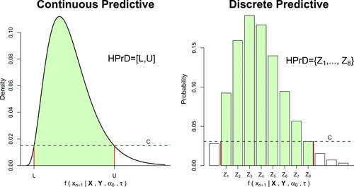
The PCC is based on the sequentially updated form of the predictive distribution, which is used to determine a region ($R_{n+1}$), where the future observable ($X_{n+1}$) will most likely be, as long as the process is stable (i.e., no changes occurred). The region $R_{n+1}$ will be the $100(1-\alpha )\%$ Highest Predictive Density (HPrD) region, which is the unique shortest region, that minimizes the absolute difference with the predetermined coverage. We will adopt the name HPrD, even for cases in which the predictive distribution is discrete, where we derive the Highest Predictive Mass (HPrM) region (see Appendix B for the strict definition of HPrD/M and details in deriving the HPrD region from a continuous or discrete distribution). PCC will plot the sequentially updated HPrD region versus time, providing the “in control” region of the next data point and thus give an alarm if a new observable does not belong to the respective HPrD region. For unimodal predictive distributions, the region $R_{n+1}$ will be an interval for continuous distributions, or a set with consecutive numbers for the discrete case, while for a multimodal predictive, $R_{n+1}$ might be formed as a union of non-overlapping regions.

2.1. On selecting $\mathit{\alpha }$

The (predetermined) parameter $0<\alpha <1,$ also known as False Alarm Rate (FAR), will reflect our tolerance to false alarms and consequently the detection power. The proposed PCC can be viewed as a sequential (multiple) hypothesis testing procedure, where at each time point n we draw the HPrD region ($R_{n+1}$) for the future observable, so that if no changes occurred in the process (IC state), the probability to raise an alarm is: $P(X_{n+1}\notin R_{n+1}|IC)=\alpha .$ We suggest two metrics in selecting α, depending on whether we know or not in advance the number of data points, N, that PCC will be used for (in short runs or Phase I studies) and/or whether N is large.

If we have a (known) fixed horizon of N data points, for which PCC will be employed and N is not too large (typically up to a few dozens), then we suggest to control the Family Wise Error Rate (FWER), which expresses the probability of raising at least one false alarm out of a pre-determined number of N hypothesis tests. This is identical to the concept of False Alarm Probability (FAP) introduced by Chakraborti, Human, and Graham (2008) for phase I analysis. Among various proposals in controlling FWER, we adopt the Šidák’s correction (Šidák 1967), which is slightly more powerful than the popular Bonferroni’s correction (Dunn 1961). Šidák’s correction assumes independence across tests and is more conservative in the presence of positive dependence, compared with independent tests. If we define V to be the number of false alarms observed in a PCC, applied on N observations in total, i.e., $n=1,\dots ,N,$ from the IC state of the distribution ($0\le V\le N-1,$ when PCC starts at n = 2), then the Šidák’s correction (assuming independence) will provide: (9) $$\begin{array}{c}F\mathit{WER}=P\left(V\ge 1\right)=1-P\left(V=0\right)=1-P\left(\underset{i=2}{\overset{N}{\cap }}\left\{X_i\in R_i|IC\right\}\right)\\ =1-\prod _{i=2}^{N}P\left(X_i\in R_i|IC\right)=1-{\left(1-\alpha \right)}^{N-1}\Rightarrow \alpha =1-{(1-\mathit{FWER})}^{\frac{1}{N-1}}.\end{array}$$(9)

So, once we know N and we set the desirable FWER, we can obtain the parameter α needed in deriving the HPrD regions, $R_{n+1}.$ It is evident that as N increases, α decreases and approaches zero, it leads to an extremely conservative decision scheme, that will reduce the OOC detection power.

We recommend to use the above approach, as long as $\alpha \ge {10}^{-3},$ even though this can be adjusted depending on the type of process we monitor. However, in the cases where N is either unknown in advance or it is too large, then we suggest to derive α using the metric of IC Average Run Length (ARL₀). Following Montgomery (2009), this corresponds to the desired average number of data points that we will plot in the PCC before a false alarm occurs, given that the process is under the IC state. As N increases, the updated posterior distribution gets more informative (offering consistent estimates of the unknown parameters) and thus the resulting hypothesis tests will tend to be nearly independent. Then, the value of the desired (predetermined) ARL₀ will be approximately: (10) $$AR{L}_0\approx \frac{1}{\alpha }\Rightarrow \alpha \approx \frac{1}{AR{L}_0}.$$(10)

Based on either (9) or (10), we predetermine the coverage level $100(1-\alpha )\%$ that the HPrD region ($R_{n+1}$) will have.

2.2. Fast initial response (FIR) PCC

One of the most serious issues in self-starting methods, is the weak response to early shifts (Goedhart, Schoonhoven, and Does 2017; Capizzi and Masarotto 2020). The Fast Initial Response (FIR) feature is typically used to improve the performance of the standard charts for early shifts in a process. Lucas and Crosier (1982) were the first to propose a FIR feature for CUSUM, while Steiner (1999) introduced the FIR EWMA by narrowing the control limits. In the latter, the time dependent effect of the FIR adjustment, decreases exponentially with time and becomes negligible after a few observations. Precisely, Steiner’s adjustment is given by: (11) $${\text{FIR}}_{\mathit{adj}}=1-{\left(1-f\right)}^{1+\mathrm{a}(t-1)},$$(11) where $\mathrm{a}>0$ is a smoothing parameter, t is the current number of hypotheses tests performed and $0<f<1$ represents the proportion of the adjusted limit over the initial test (i.e., t = 1).

As the PCC uses control limits, much like the EWMA, we will adopt Steiner’s adjustment for a time-varying narrowing of the $R_{n+1}$ region in the start of the process. Despite the head-start the FIR option can provide to PCC, we should make sure that we do not significantly inflate the false alarms. Thus, the FIR parameters should be selected by taking into account the false alarm behavior of PCC, which depends on the prior settings, especially when the volume of available data is small. If an extremely informative prior (near point mass) is used, then the PCC behavior acts like a typical Shewhart chart, as the resulting $R_{n+1}$ region is not essentially updated by new observations. On the other hand, if a non-informative prior, like the initial reference prior without historical IC data, is selected, then the FAR depends only on the (iid) data. As a result for these two cases, the observed FAR will meet the predetermined standards (even from the very first hypothesis test) and therefore we should avoid the use of a FIR adjustment (or otherwise the observed FAR will be inflated).

However, in the case of a weakly informative prior, the $R_{n+1}$ region is quite wide (as we combine prior and likelihood uncertainty), but at the same time the prior distribution provides beneficial information for the IC state. Combining these two facts, the first IC data points are more likely to be plotted within the $R_{n+1}$ region. This will result in a temporarily smaller (from what is anticipated) FAR, especially for the very early tests at the start of a process. Thus, we could use a FIR adjustment without a negative effect on the predetermined expected number of false alarms. We propose to be somewhat conservative and use f = 0.99, i.e., the adjusted $R_{n+1}$ region will be the 99% of the original for the first test and $\mathrm{a}=(-3/lo{g}_{10}(1-f)-1)/4,$ i.e., the adjusted $R_{n+1}$ region will be the 99.9% of the original at the fifth test. We should note that t is the current number of tests, not the number of observations, as for the first (or the second) observation PCC does not provide a test.

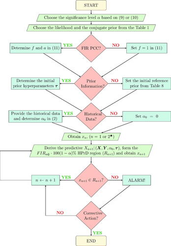
A flowchart in Figure 1 synopsizes the general PCC scheme with all possible options of its implementation, while in Appendix C we present it in a form of an algorithm.

Figure 1. PCC flowchart. A parallelogram corresponds to an input/output information, a decision is represented by a rhombus and a rectangle denotes an operation after a decision making. In addition, the rounded rectangles indicate the beginning and end of the process.

^★For the Normal – NIG model using the initial reference prior and ${\alpha }_0=0$ we need n = 2 to initiate PCC, while for all other cases PCC starts once x₁ becomes available.

3. PCC based decision making

The major role of PCC is to control a process and identify transient large shifts (outliers), in an online fashion and without a phase I exercise. As such, PCC performs a hypothesis test as each new data point $x_{n+1}$ becomes available and raises an alarm when $x_{n+1}\notin R_{n+1},$ indicating that the new observable is not in agreement with what is anticipated from the predictive distribution (that was built from the previous data and the prior distribution). The endpoints of $R_{n+1},$ formed from the predictive distribution, play the role of the control limits of the chart. The range of these limits reflect the variability of the predictive distribution, which is known to depend on both the length of the available data and the precision of the prior distribution. For a weakly informative prior the range will be wider at the start of the process and as more data become available it will become more narrow and eventually stabilize, washing out the effect of the prior. Figure 2 provides illustrations of PCC for data streams of length 30 that come from a continuous (Normal data with both parameters unknown) and two discrete (Poisson and Binomial) cases, when the process is either IC or has a large isolated shift at location 15 (OOC scenario).

Figure 2. The IC and OOC illustration of PCC for Normal, Poisson and Binomial data. For the IC Normal data $X_i|({\theta }_1,{\theta }_2^2)\stackrel{\mathit{iid}}{\sim }N({\theta }_1=0,{\theta }_2^2=1)$ and for the OOC case we sample $X_{15}\sim N(4,1).$ The initial prior was $({\theta }_1,{\theta }_2^2)\sim \mathit{NIG}(\mu =0,\lambda =2,a=1,b=0.8).$ For the IC Poisson data $X_i|{\theta }_3\stackrel{\mathit{iid}}{\sim }P({\theta }_3=4).$ For the OOC case $X_{15}\sim P(10),$ while ${\theta }_3\sim G(c=8,d=2).$ For the IC Binomial data $X_i|{\theta }_4\stackrel{\mathit{iid}}{\sim }Bin(N=20,{\theta }_4=0.1).$ For the OOC case $X_{15}\sim \mathit{Bin}(20,0.368),$ while ${\theta }_4\sim \mathit{Beta}(a=0.5,b=4.5).$ In all cases, α needed to derive the $100(1-\alpha )\%$ HPrD $(R_{n+1})$ was selected to satisfy FWER = 0.05 for N = 30 observations.

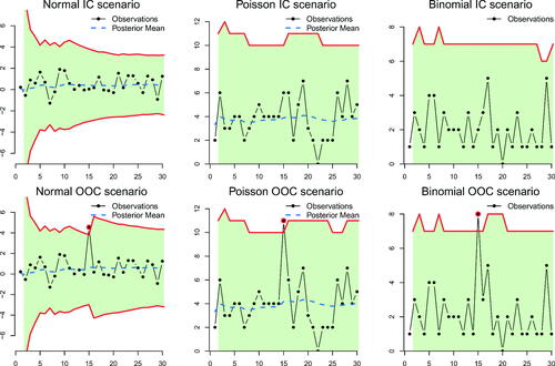
As can be seen in Figure 2, the limits tend to become more narrow and finally stabilize when the size of the data increases, forming a more informative posterior distribution of the unknown parameter(s). The outlying observations in all scenarios are plotted outside the $R_{n+1}$ region, hence raising an alarm. The region $R_{n+1}$ is formed online, after the data point x_n becomes available, and so when we get an alarm (i.e., $x_{n+1}\notin R_{n+1}$), the suggestion is to stop the process, perform some root cause analysis to identify external sources of variation, possibly have an intervention and finally restart the PCC (the posterior we had right before the alarm can act as the new prior, or the previous IC data can be used in the power prior mechanism). However, if we will not react to an alarm, due to the Bayesian dynamic update mechanism, the isolated change detected will be absorbed. As a consequence, the posterior and predictive distribution will have inflated variance leading to wider $R_{n+1}$ regions. In the OOC scenarios in Figure 2 we observe that the $R_{n+1}$ regions are wider at time 16 due to the “no action” policy at the alarm for time 15. This effect is reduced with time but it is still present until observation 30, where the $R_{n+1}$ is wider compared to the respective region of the IC data.

Apart from controlling a process, PCC can be used for monitoring the unknown parameter(s). As we showed in Theorem 1, before deriving the predictive distribution at each time point, we first obtain the posterior distribution for the unknown parameter(s). Decision theory can be used to provide loss function based optimal point/interval estimates and/or hypothesis testing for each parameter. For example, using the squared error loss function, the Bayes rule (optimal point estimate) is known to be the mean of the posterior distribution (Carlin and Louis 2009), i.e., we have a (sequentially updated) point estimate of the unknown process parameter(s). To illustrate this option, in Figure 2, we additionally plot the posterior mean estimate of θ₁ for the Normal and θ₃ for the Poisson cases.

Finally, PCC summarizes the predictive distribution through a region, but other forecasting options (like point estimates) are straightforward to derive as well using decision theory.

4. Competing methods and sensitivity analysis

The PCC is developed in a general framework, allowing its use for any likelihood that belongs to the k-PREF. In traditional SPC/M, significant amount of work has been dedicated for Normal, Poisson and Binomial data. When the goal is to detect transient large shifts in a short run process of individual univariate data, without employing a phase I calibration stage, the Q-charts developed by Quesenberry (1991a, 1991b, 1991c) are probably the most prominent representative methods for Normal, Binomial and Poisson data respectively. In absence of phase I parameter estimates, the Q-charts provide a self-starting monitoring method, where calibration and testing happens simultaneously, aiming to detect process disturbances (OOC states) in an online fashion.

In this section we will compare the performance of the proposed PCC methodology against Q-chart for Normal, Poisson and Binomial data, i.e., a Bayesian versus a frequentist parametric approach. For the latter and precisely in the case of Normal data, Quesenberry (1991a) presented three versions of Q-chart (we ignore the scenario that both parameters are known) when either a parameter is known or both unknown, for which we have the following:

Lemma 2.

All three versions of Q-Chart for Normal data are special cases of the respective PCCs, when the initial prior is the reference prior and we do not make use of a power prior option (i.e., ${\alpha }_0=0$).

Appendix D provides the proof of this lemma, which shows that the Normal Q-charts (in all three cases) are identical to the respective PCC when neither prior information (i.e., use of reference prior) nor historical data are available. What happens though when prior information and/or historical data do exist? In such scenarios, the posterior distribution will be more informative, enhancing the predictive distribution, which will boost the PCC performance. For discrete data (Poisson and Binomial) the Q-charts use the uniform minimum variance unbiased (UMVU) estimation of the cumulative distribution function of the process, thus we lose ability to compare analytically against the respective exact discrete PCC.

In what follows we will perform a simulation study to examine the performance of Q-charts against PCC when we have N = 30 data points from $N({\theta }_1,{\theta }_2^2),P({\theta }_3)$ or $\mathit{Bin}(20,{\theta }_4)$ distributions. We will design charts to have a FWER = 0.05 at the last observation N = 30 (using Šidák correction). We will compare the running $\mathit{FWER}(k)=1-P({\cap }_{i=2}^k\left\{X_i\in R_i|IC\right\})$ of Q-charts and PCC at each of the $k=2,\dots ,30$ data points, when we simulate IC sequences from $N({\theta }_1=0,{\theta }_2^2=1),P({\theta }_3=2)$ and $\mathit{Bin}(20,{\theta }_4=0.1)$ respectively (see Keefe, Woodall, and Jones-Farmer 2015 for more details regarding the conditional IC performance of self-starting control charts). To examine the OOC detection power of Q-charts and PCC we will use the IC sequences generated and introduce large isolated shifts at one of the locations: 5 (early), 15 (middle) or 25 (late). The size of the shifts that we will consider are:

• Normal mean: ${\delta }_N=\left\{2.5{\theta }_2\mathrm{ }\text{or}\mathrm{ }3{\theta }_2\right\}=\left\{2.5\mathrm{ }\text{or}\mathrm{ }3\right\},$ i.e., OOC states come from $N(2.5,1)$ or N(3, 1).

• Poisson mean (or variance): ${\delta }_P=\left\{2.5\sqrt{{\theta }_3}\mathrm{ }\text{or}\mathrm{ }3\sqrt{{\theta }_3}\right\}=\left\{2.5\sqrt{2}\mathrm{ }\text{or}\mathrm{ }3\sqrt{2}\right\},$ i.e., OOC states come from $P(2+2.5\sqrt{2})=P(5.536)$ or $P(2+3\sqrt{2})=P(6.243).$

• Binomial probability of succes: ${\delta }_B=\{2.5\sqrt{\frac{{\theta }_4(1-{\theta }_4)}{N}}\mathrm{ }\text{or}\mathrm{ }3\sqrt{\frac{{\theta }_4(1-{\theta }_4)}{N}}\}=\{2.5\sqrt{\frac{0.1(1-0.1)}{20}}\mathrm{ }\text{or}\mathrm{ }3\sqrt{\frac{0.1(1-0.1)}{20}}\},$ i.e., OOC states come from $\mathit{Bin}(20,0.268)$ or $\mathit{Bin}(20,0.301).$

For detection, we will record the cases that a chart provides an alarm at the exact time that the shift was introduced. More specifically, these cases will be denoted as the OOC Detection (OOCD), where $\mathit{OOCD}(k^{\prime })=P(\left\{X_{k^{\prime }}\notin R_{k^{\prime }}|\mathit{OOC}\right\}{\cap }_{i=2}^{k^{\prime }-1}\left\{X_i\in R_i|IC\right\}),$ where $k\prime =\{5,15,25\}.$ Both $\mathit{FWER}(k)\%$ for IC data (at each time 2, …, 30) and $\mathit{OOCD}(k\prime )\%$ at locations 5, 15, or 25 will be estimated over 100,000 iterations.

PCC will require to define a prior distribution and so within this simulation study we will take advantage to examine the sensitivity of the PCC performance for various prior settings. Precisely, for each setup described above, we will make use of two initial priors (reference and weakly informative) and two values for the α₀ parameter (0 or $1/n_0$) representing the absence or presence of n₀ historical data Y (we will use $n_0=10$ historical data from the IC likelihood). Therefore, for each scenario we will compare the Q-chart against one of the four possible versions of PCC (with/without prior knowledge, with/without historical data). The initial priors ${\pi }_0(·|\mathit{\tau }),$ which we will employ are (see Figure 3):

Figure 3. The initial reference (i.e., non-informative) and the weakly informative prior distributions used in the simulation study, along with the IC values (as vertical segments) for the parameters ${\theta }_1,{\theta }_2^2,{\theta }_3$ and θ₄ of the simulation study.

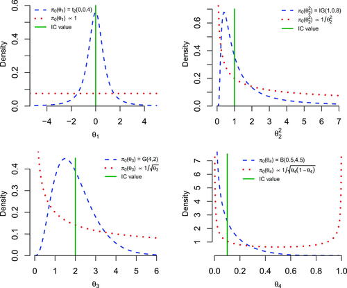
• Normal: reference prior ${\pi }_0({\theta }_1,{\theta }_2^2)\propto 1/{\theta }_2^2\equiv \mathit{NIG}(0,0,-1/2,0)$ or the weakly informative $\mathit{NIG}(0,2,1,0.8).$

• Poisson: reference prior ${\pi }_0({\theta }_3)\propto 1/\sqrt{{\theta }_3}\equiv G(1/2,0)$ or the weakly informative G(4, 2).

• Binomial: reference prior ${\pi }_0({\theta }_4)\propto 1/\sqrt{{\theta }_4(1-{\theta }_4)}\equiv \mathit{Beta}(1/2,1/2)$ or the weakly informative $\mathit{Beta}(0.5,4.5).$

The simulation findings are summarized graphically in Figure 4 and analytically in Table 2, where we observe that overall PCC outperforms Q-chart. Starting from the false alarms in the case of Normal data, both methods reach the nominal 5% at time N = 30, but at all time points k, the FWER(k) of PCC is always smaller. For both discrete cases, the Q-chart’s FWER(k) becomes unacceptably high, something that is caused from the fact that the true parameter values are near (even though not too close) to the parameter space boundary, which in conjunction with the UMVU estimation, inflates drastically the false alarms (the closer we get to the parameter boundary the worst the performance regarding false alarms). Finally, the extremely small FWER(k) observed for PCC in the first 5 data points motivates the use of the FIR-PCC described in Section 2.2.

Figure 4. The FWER(k) at each time point $k=2,3,\dots ,30$ (top row) and the $\mathit{OOCD}(k\prime )$ at $k\prime =5,15,$ or 25, of the Q-chart and PCC under a reference prior (PCC₁), a reference prior with historical data $(PC{C}_2),$ a weakly informative prior (PCC₃) and a weakly informative prior with historical data $(PC{C}_4),$ when we have outliers of 2.5 (middle row) or 3 (bottom row) standard deviations. Columns 1 to 3 refer to the Normal, Poisson and Binomial cases respectively.

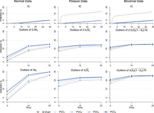
Table 2. The FWER for N = 30 (in parenthesis) and the outlier detection power at $k\prime =\{5,15,25\},$ of the Q-chart against PCC under a reference prior (PCC₁), a reference prior with historical data $(PC{C}_2),$ a weakly informative prior (PCC₃) and a weakly informative prior with historical data $(PC{C}_4).$

			Q-chart	PCC1	PCC2	PCC3	PCC4
			$\mathit{OOCD}(k\prime )\%$	$\mathit{OOCD}(k\prime )\%$	$\mathit{OOCD}(k\prime )\%$	$\mathit{OOCD}(k\prime )\%$	$\mathit{OOCD}(k\prime )\%$
	Jump	$k\prime$	($\mathit{FWER}\%$)	($\mathit{FWER}\%$)	($\mathit{FWER}\%$)	($\mathit{FWER}\%$)	($\mathit{FWER}\%$)
Normal	$0\sigma$		(5.049)	(5.049)	(4.347)	(4.776)	(4.932)
		5	1.901	1.901	1.492	4.205	6.271
	$2.5\sigma$	15	12.791	12.791	14.249	17.433	18.407
		25	17.025	17.025	17.691	20.005	20.371
		5	2.873	2.873	2.816	9.024	12.556
	$3\sigma$	15	22.809	22.809	24.914	30.112	31.426
		25	30.095	30.095	31.021	34.410	34.880
Poisson	$0\sqrt{\lambda }$		(18.283)	(4.515)	(4.192)	(4.409)	(4.320)
		5	12.437	12.696	14.793	16.265	16.928
	$2.5\sqrt{\lambda }$	15	17.220	18.196	18.660	19.052	19.302
		25	17.704	19.164	19.180	19.510	19.623
		5	18.185	19.185	21.984	24.240	25.204
	$3\sqrt{\lambda }$	15	24.930	26.826	27.434	27.972	28.345
		25	25.740	28.153	28.196	28.683	28.823
Binomial	$0\sqrt{\frac{p(1-p)}{N}}$		(17.878)	(4.387)	(3.991)	(4.852)	(4.381)
		5	14.079	15.848	15.540	16.111	17.008
	$2.5\sqrt{\frac{p(1-p)}{N}}$	15	20.057	18.845	19.319	20.084	20.067
		25	20.284	19.878	20.035	19.839	20.315
		5	21.646	24.078	24.098	24.509	26.039
	$3\sqrt{\frac{p(1-p)}{N}}$	15	29.469	28.765	29.353	30.207	30.213
		25	29.952	30.165	30.389	30.117	30.703

The results refer to Normal, Poisson and Binomial data.

For the Normal data, the simulations verify Lemma 2, as the Q-chart and the PCC with reference prior and no historical data have identical performance. Moving to the detection power, as it is measured by $\mathit{OOCD}(k\prime ),$ both methods improve as the size of the shift increases (from 2.5 to 3 sd) or the shift delays its appearance (from $k\prime =5$ to 15 to 25), just as it was expected. Especially for the shifts at time 5, PCC greatly outperforms Q-charts thanks to the head-start from the prior and/or the historical data. Focusing at each location of the shift, we observe that as we move from Q-chart to PCC with reference prior and next to PCC with weakly informative prior the performance improves (quite significantly for some scenarios). When relevant historical data are available, through the power prior mechanism, they further boost the performance. The somewhat competitive performance of Q-chart in one of the Binomial scenarios should be considered in conjunction with its quite high FWER, when compared to the one achieved by PCC (see also Table 3, where the FWER of PCCs is increased to align with the one that Q-chart can achieve in the Poisson and Binomial cases, offering a straightforward comparison of detection power). In summary, PCC appears more powerful to the respective Q-charts in detecting isolated shifts in short runs of individual data.

Table 3. The FWER for N = 30 (in parenthesis) and the outlier detection power at $k\prime =\{5,15,25\},$ of the Q-chart against PCC under a reference prior (PCC₁), a reference prior with historical data $(PC{C}_2),$ a weakly informative prior (PCC₃) and a weakly informative prior with historical data $(PC{C}_4).$

			Q-chart	PCC1	PCC2	PCC3	PCC4
			$\mathit{OOCD}(k\prime )\%$	$\mathit{OOCD}(k\prime )\%$	$\mathit{OOCD}(k\prime )\%$	$\mathit{OOCD}(k\prime )\%$	$\mathit{OOCD}(k\prime )\%$
	Jump	$k\prime$	($\mathit{FWER}\%$)	($\mathit{FWER}\%$)	($\mathit{FWER}\%$)	($\mathit{FWER}\%$)	($\mathit{FWER}\%$)
Poisson	$0\sqrt{\lambda }$		$(18.283)$	$(16.498)$	$(15.646)$	$(16.550)$	$(16.183)$
		5	18.185	34.295	35.388	38.820	39.221
	$2.5\sqrt{\lambda }$	15	24.930	38.634	39.192	39.899	40.388
		25	25.740	37.823	38.215	38.456	38.679
		5	12.437	25.410	26.138	28.906	29.157
	$3\sqrt{\lambda }$	15	17.220	28.657	29.108	29.736	30.166
		25	17.704	28.181	28.440	28.692	28.869
Binomial	$0\sqrt{\frac{p(1-p)}{N}}$		$(17.878)$	$(16.606)$	$(15.383)$	$(17.950)$	$(16.682)$
		5	21.646	38.442	38.898	38.345	40.992
	$2.5\sqrt{\frac{p(1-p)}{N}}$	15	29.469	40.947	42.666	42.406	43.004
		25	29.952	40.052	41.283	40.589	41.210
		5	14.079	28.073	28.037	27.982	29.906
	$3\sqrt{\frac{p(1-p)}{N}}$	15	20.057	29.549	30.984	30.920	31.351
		25	20.284	29.040	30.053	29.662	30.039

The results refer to Poisson and Binomial data, where PCC has aligned FWER with the one achieved by Q-chart.

Focusing on the performance of PCC at location $k\prime =5,$ we observe that in the Normal scenario we have smaller power compared to the respective setting in Poisson or Binomial (as we move $k\prime$ to higher values, the differences vanish). This is caused from the fact that in the Normal scenario we have two unknown parameters as opposed to the Poisson and Binomial cases where each has only one unknown parameter (a PCC built using four data points for a setting with two unknown parameters will be a lot more challenging, as opposed to a setting with only one unknown parameter). A Normal PCC scheme with either the mean or the variance being known would radically improve the performance reaching (or even overcoming) the levels achieved in the Poisson and Binomial. The effect of the two unknown parameters (Normal) versus the single unknown parameter (Poisson and Binomial) is responsible in the performance of PCC₁ to PCC₄ in detecting outliers at $k\prime =25.$ With one unknown parameter, the information collected from the 24 in control data points has significantly reduced the posterior (and predictive) uncertainty, shrinking the effect of the prior and providing a near uniform performance. For the Normal case though the posterior (and predictive) uncertainty at $k\prime =25$ remains non-negligible, allowing the prior setting to play some role and differentiate the performance across the four versions of PCCs (in general the more the data the higher the shrinkage of the prior’s effect).

Regarding the prior sensitivity and its effect on the PCC performance (emphasizing in Normal, Poisson and Binomial data), a more thorough discussion along with certain guidelines on prior elicitation can be found in Appendix E. Wrapping up this section, we should note that PCC was shown to be more powerful in detecting large isolated shifts compared to Q-chart. The relative performance of Q-chart to PCC remains the same when we use medium or small shifts, with detection power dropping as the size of the isolated shift decreases.

5. Robustness

Apart from checking the prior sensitivity that was done in Section 4, we will also examine how robust the suggested PCC performance is to possible model type misspecifications. For the PCC construction we assume that the observed data are iid observations from a specific likelihood. In this section, we will examine how robust is the PCC performance when:

1. we violate the assumption of independence (i.e., the data are correlated)

2. the assumed likelihood function is invalid (i.e., data are generated from a different random variable from the one assumed in the PCC construction).

Regarding (a) we will use a Normal (with both parameters unknown) PCC implementation, but the actual data will be generated as sequentially dependent Normal data via an autoregressive (AR) model: $X_n=c+\varphi X_{n-1}+{ϵ}_n$ with c = 0 and ${ϵ}_n\sim N(0,1).$ To examine various degrees of dependence we will use $\varphi =-0.4,0.4$ (moderate) or 0.8 (high). For the outlying observations we will set $c=$ 2.5 or 3, in order to introduce shifts of size of $2.5\sigma$ or $3\sigma$ respectively, at one of the locations 5, 15 or 25 (just as we did in Section 4).

For (b) we will examine the following scenarios:

• Use a Normal based PCC (both parameters unknown) while the data are generated from a Student t₇ distribution, i.e., we have heavier tails (t₇ is symmetric, with the same mean but 40% inflated variance compared with the standard Normal).

• Use a Normal based PCC (both parameters unknown) while the data are generated from a $\mathit{Gumbel}(\mu =-0.5,\beta =0.8)$ distribution, i.e., we have skewed data ($Gu(-0.5,0.8)$ has approximately the same mean and variance with the standard Normal, but it has positive skewness $\approx 1.14$).

• Use a Poisson based PCC while the data are generated from a $\mathit{NBin}(r=6,p=1/4)$ distribution, i.e., we have over-dispersed data ($\mathit{NBin}(6,1/4)$ has the same mean with P(2), but its variance is $\approx 33\%$ inflated).

The aforementioned likelihoods are illustrated in Figure 5. For this misspecification scenario, we generate the OOC data from the introduced distributions in a manner that the isolated large shifts will correspond to either 2.5 or 3 standard deviations, again at locations 5, 15 or 25 (similar to what we had in Section 4). Precisely:

Figure 5. The various misspecification of the PCC distributional forms regarding the continuous (left panel) and discrete (right panel) data generation mechanisms.

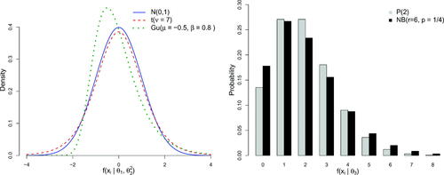
• Student t: OOC states come from $t_7\left(\mu =2.5·\sqrt{7/5},\sigma =1\right)$ or $t_7\left(\mu =3·\sqrt{7/5},\sigma =1\right).$

• Gumbel: OOC states come from $Gu(-0.5+2.5,0.8)$ or $Gu(-0.5+3,0.8).$

• Negative Binomial: OOC states come from $\mathit{NBin}(6·2.5,1/4)$ or $\mathit{NBin}(6·3,1/4).$

The prior distributions (reference prior and weakly informative) along with the use or not of $n_0=10$ historical data (power prior with ${\alpha }_0=0\mathrm{ }\text{or}\mathrm{ }1/n_0$) will be identical to the ones used in Section 4.

Figures 6 and 7 summarize graphically the results of Tables 4 and 5, regarding the performance (FWER(k) and $\mathit{OOCD}(k\prime )$ are as defined in Section 4) for independence and distributional misspecifications respectively. In the former, we observe that PCC is almost unaffected in the presence of moderate autocorrelation. For highly dependent data ($\varphi =0.8$ or larger), PCC is somewhat less robust as it decreases its detection power and slightly increases the FWER percentages, however still achieving noticeable performance, especially at the early stages thanks to the IC prior information.

Figure 6. The FWER(k) at each time point $k=2,3,\dots ,30$ (top row) and the $\mathit{OOCD}(k\prime )$ at $k\prime =5,15,$ or 25 and size of 2.5 (middle row) or 3 (bottom row) standard deviations for the Normal distribution PCC with both parameters being unknown, when we actually have data from an AR(1) process. A reference or weakly informative prior and the presence or absence of historical data is considered. Columns 1 to 3 refer to the various degrees of autocorrelation.

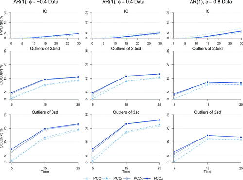
Figure 7. The FWER(k) at each time point $k=2,3,\dots ,30$ (top row) and the $\mathit{OOCD}(k\prime )$ at $k\prime =5,15,$ or 25, of PCC under a reference or weakly informative prior and in the presence or absence of historical data, when we have outliers of 2.5 (middle row) or 3 (bottom row) standard deviations. Columns 1 and 2 refer to the Normal PCC with both parameters being unknown while the data come from a Student or Gumbel distribution respectively. In column 3 we assume Poisson based PCC while the data are from a Negative Binomial.

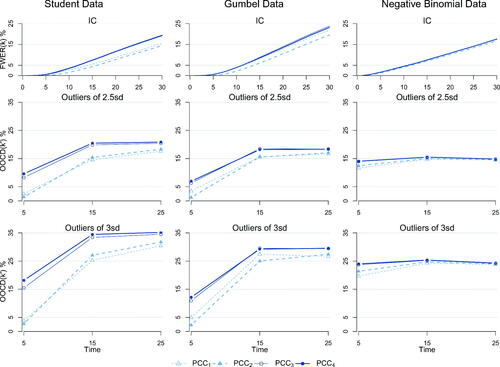
Table 4. The FWER at N = 30 (in parenthesis) and the outlier detection power at $k\prime =\{5,15,25\}$ for the Normal distribution for PCC with both parameters being unknown, when we actually have data from an AR(1) process.

			PCC1	PCC2	PCC3	PCC4
			$\mathit{OOCD}(k\prime )\%$	$\mathit{OOCD}(k\prime )\%$	$\mathit{OOCD}(k\prime )\%$	$\mathit{OOCD}(k\prime )\%$
	Jump	$k\prime$	($\mathit{FWER}\%$)	($\mathit{FWER}\%$)	($\mathit{FWER}\%$)	($\mathit{FWER}\%$)
A R (1), $\varphi =-0.4$	0sd		(4.420)	(3.293)	(4.711)	(4.480)
		5	1.421	0.511	4.038	4.789
	$2.5sd$	15	9.822	10.369	14.050	14.441
		25	13.289	13.794	15.995	16.270
		5	2.059	1.066	8.092	9.880
	3sd	15	17.294	18.516	24.093	24.776
		25	23.557	24.446	27.724	28.185
A R (1), $\varphi =0.4$	0sd		(6.319)	(4.135)	(5.530)	(5.026)
		5	2.535	0.531	4.082	4.755
	$2.5sd$	15	12.724	12.915	16.640	16.669
		25	15.511	15.943	18.120	18.308
		5	3.671	1.155	8.615	10.138
	3sd	15	21.836	22.571	28.115	28.342
		25	26.773	27.656	30.740	31.135
A R (1), $\varphi =0.8$	0sd		(9.218)	(5.637)	(7.226)	(6.795)
		5	3.098	0.347	3.135	3.854
	$2.5sd$	15	11.237	10.191	12.407	12.121
		25	10.341	10.509	11.668	11.640
		5	4.591	0.857	6.508	7.904
	3sd	15	17.783	16.820	20.031	19.832
		25	16.488	16.931	18.619	18.712

PCC process is under a reference prior (PCC₁), a reference prior with historical data $(PC{C}_2),$ a weakly informative prior (PCC₃) and a weakly informative prior with historical data $(PC{C}_4).$

Table 5. The FWER at N = 30 (in parenthesis) and the outlier detection power at $k\prime =\{5,15,25\}$ for the Normal distribution for PCC violating the distributional assumption.

			PCC1	PCC2	PCC3	PCC4
			$\mathit{OOCD}(k\prime )\%$	$\mathit{OOCD}(k\prime )\%$	$\mathit{OOCD}(k\prime )\%$	$\mathit{OOCD}(k\prime )\%$
	Jump	$k\prime$	($\mathit{FWER}\%$)	($\mathit{FWER}\%$)	($\mathit{FWER}\%$)	($\mathit{FWER}\%$)
t – S t u d e n t (df = 7)	0sd		$(15.338)$	$(14.425)$	$(19.128)$	$(19.361)$
		5	2.543	1.366	8.282	9.606
	$2.5sd$	15	14.576	15.417	19.861	20.468
		25	17.560	18.313	20.427	20.847
		5	3.782	2.737	15.511	18.167
	3sd	15	25.243	27.059	33.409	34.462
		25	30.435	31.765	34.518	35.183
G u m b e l $(\mu =-0.5,\beta =0.8)$	0sd		$(21.903)$	$(19.583)$	$(23.849)$	$(23.227)$
		5	3.488	1.245	6.320	6.953
	$2.5sd$	15	15.614	15.528	18.505	18.180
		25	16.654	17.021	18.387	18.333
		5	4.911	2.279	10.943	12.150
	3sd	15	27.444	25.030	29.539	29.259
		25	26.648	27.426	29.420	29.549
N e g. B i n $\left(r=6,p=\frac{1}{4}\right)$	0sd		$(17.526)$	$(16.761)$	$(17.686)$	$(17.543)$
		5	11.626	12.478	13.976	14.055
	$2.5sd$	15	14.766	15.035	15.442	15.504
		25	14.499	14.601	14.772	14.848
		5	19.709	21.374	23.701	24.010
	3sd	15	24.251	24.690	25.254	25.351
		25	23.790	23.997	24.171	24.290

Panel 1 and 2 refer to the Normal PCC with both parameters being unknown while the data come from a Student or Gumbel distribution respectively. In panel 3 we assume Poisson based PCC while the data are from a Negative Binomial. PCC process is under a reference prior (PCC₁), a reference prior with historical data $(PC{C}_2),$ a weakly informative prior (PCC₃) and a weakly informative prior with historical data $(PC{C}_4).$

In the distributional violation scenarios (Figure 7), we observe that PCC retains its high detection percentages in all cases. However, the FWER(k) is significantly inflated. This can be explained by considering the shape discrepancies among the assumed and actual likelihood functions, where IC values are somewhat outlying under the misspecified assumed model (a more strict α value in determining the HPrD region would reduce the FWER(k) in such scenarios at the cost of somewhat reducing power).

Finally, for both the violation schemes, it is worth mentioning that PCC detection seems to be stabilized and not necessarily improved when the outliers occur at location 25. This can be attributed to the contaminated estimates of the unknown parameters from the data that violate the PCC assumptions, as well as the fact that the influence of the prior is decreased. Overall, the PCC appears to be robust when we violate the assumptions, as its performance is somewhat reduced but noticeably far from collapsing.

6. Real data application

In this section we will illustrate the use of PCC in practice. Specifically, we will apply the proposed PCC methodology in two real data sets (one for continuous and one for discrete data). Regarding the continuous case, we will use data that come from the daily Internal Quality Control (IQC) routine of a medical laboratory. We are interested in the variable “activated Partial Thromboplastin Time” (aPTT), measured in seconds. APTT is a blood test that characterizes coagulation of the blood. It is a routine clotting time test and can be used as a diagnosis of bleeding risk (e.g., aPTT value is higher in patients with hemophilia or Willebrand disease) or for unfractionated heparin treatment monitoring. We gathered 30 daily normal IQC observations (X_i) from a medical lab (see Table 6), where $X_i|({\theta }_1,{\theta }_2{}^2)\sim N({\theta }_1,{\theta }_2{}^2).$ Notice that these data are based on control samples and in regular practice will become available sequentially. The goal is to accurately detect any transient parameter shift of large size, as this will have an impact on the reported patient results. Thus, it is of major importance to perform on-line monitoring of the process without a phase I exercise. Via available prior information, we elicit the prior ${\pi }_0({\theta }_1,{\theta }_2{}^2|\mathit{\tau })\sim \mathit{NIG}(29.6,1/7,2,{0.56}^2).$ Furthermore, there were $n_0=30$ historical data (from a different reagent) available (see Table 6), with $\overline{\mathbf{y}}=30.18$ and $\mathit{var}(\mathbf{y})=0.32.$ We set ${\alpha }_0=1/30$ and combining these two sources of information we get the power prior $\pi ({\theta }_1,{\theta }_2{}^2|\mathit{Y},{\alpha }_0,\mathit{\tau })\sim \mathit{NIG}(30.1,8/7,5/2,{0.7}^2).$ To examine prior sensitivity we will also use as initial prior the reference prior ${\pi }_0({\theta }_1,{\theta }_2{}^2|\mathit{\tau })\propto 1/{\theta }_2^2\equiv \mathit{NIG}(0,0,-1/2,0)$ (to declare a-priori ignorance) and so we will get two versions of PCC (one for each initial prior). Figure 8 provides the two versions of PCC (continuous/dotted limits for weakly informative/reference prior) along with a plot of the historical data and the marginal distributions of the mean (θ₁) and variance $({\theta }_2^2)$ at the end of the data collection. Specifically, for each parameter we plot the marginal weakly informative initial, ${\pi }_0(·|\mathit{\tau }),$ power, $\pi (·|\mathit{Y},{\alpha }_0,\mathit{\tau }),$ priors and the posterior distribution, $p(·|\mathit{X},\mathit{Y},{\alpha }_0,\mathit{\tau }).$ We should emphasize that despite the fact that we provide the plots at the end of the data sequence, in practice the PCC chart and each of the two posterior distributions will start being plotted at observation 2 and 1 respectively and will be sequentially updated every time a new observable becomes available. PCC provides an alarm at location 16, indicating that there was a transient large shift during that day. This would call for checking the process at that date and if an issue was found then we would take some corrective action, initiate the PCC and reanalyze all the patient samples that were received between days 15 (no alarm) and 16 (alarm). In the present study, no action was taken and the process continued to operate. As a result, the PCC limits were inflated right after the alarm, but this effect was gradually absorbed as more IC data become available. We also note (as expected) that the use of the reference prior provides wider limits, especially at the early stage of the process, making the chart less responsive. Finally, the marginal posterior distributions can be used to draw inference regarding the unknown parameters, at each time point.

Figure 8. The PCC application on Normal data. At the upper panels (left and right), we have the marginal distributions for the mean and the variance respectively. With the dotted, dashed and solid lines we denote the initial prior, the power prior and the posterior after gathering all the current data respectively. At the lower panels, we provide the time series of the historical data (open circles on left) and of the current data (solid points on the right). The solid lines represent the limits of PCC, the dotted lines are the limits of PCC under prior ignorance, i.e., using the initial reference prior and the dash lines correspond to the FIR adjustment, setting f = 0.99 and $\mathrm{a}=(-3/lo{g}_{10}(1-f)-1)/4=0.125.$

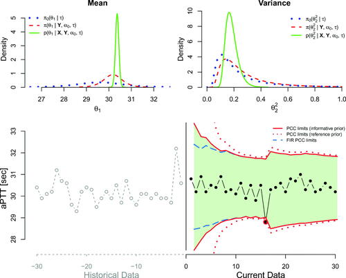
Table 6. The aPTT (in seconds) internal quality control observations of the historical $\mathit{Y}=(y_1,y_2,\dots ,y_{30})$ and the current $\mathit{X}=(x_1,x_2,\dots ,x_{30})$ data.

$y_1-y_{15}$	30.4	29.9	30.1	30.2	31.2	30.7	30.6	29.6	29.3	30.2	30.4	30.3	29.5	29.9	30.2
$x_1-x_{15}$	30.8	30.2	30.9	30.2	30.5	30.4	30.9	30.2	30.3	30.1	30.6	29.9	30.5	29.8	30.5
$y_{16}-y_{30}$	29.9	30.5	29.7	30.7	29.9	29.6	30.1	30.1	29.9	30.1	29.9	29.9	29.7	32.2	30.6
$x_{16}-x_{30}$	28.8	30.3	30.4	30.6	30.2	30.8	30.7	31.0	30.3	30.7	30.2	30.3	30.6	30.4	30.2

Next, we provide an illustration of PCC for discrete (Poisson) data. The data come from Hansen and Ghare (1987) and were also analyzed by Bayarri and García-Donato (2005). They refer to the number of defects (x_i), per inspected number of units (s_i), encountered in a complex electrical equipment of an assembly line. We have 25 counts (see Table 7) arriving sequentially that we will model using the Poisson distribution with unknown rate parameter, i.e., $X_i|\theta \sim P(\theta ·s_i).$ In contrast to the previous application, neither prior information regarding the unknown parameter nor historical data exist. Therefore, we use the reference prior as initial prior for θ, i.e., ${\pi }_0(\theta |\mathit{\tau })\propto 1/\sqrt{\theta }\equiv G(1/2,0)$ and we also set ${\alpha }_0=0$ for the power prior term. In Figure 9, we provide the initial prior and posterior distributions, the plot of the data, (daily rate of defects i.e., total number of defects per number of inspected units and number of inspected units) and the Poisson based PCC (the wavy form of the limits is caused by the variation in the number of inspected units we have per day). Similarly to what we mentioned earlier, the posterior and the PCC will start from times 1 and 2 respectively and will be updated sequentially, every time a new data point becomes available, offering online inference in controlling the process. PCC raises two alarms, at locations 13 and 25. In the former, the observed rate (30/3 = 10) seems to be higher (process degradation) from what it was expected from the process as it was evolving till that time, while the latter indicates that the observed rate (14/8 = 1.75) was smaller from what PCC was anticipating (process improvement). Similar to the previous application, the fact that the alarms were kept in the process inflated the subsequent limits. At last, online inference regarding the unknown Poisson rate parameter is available via its (sequentially updated) posterior distribution.

Figure 9. The PCC application on Poisson data. At the upper left panel we have the distributions for the rate parameter. With the dashed and solid lines we denote the prior and posterior distributions respectively, after gathering all the available data. At the upper right panel, we provide the number of inspected units s_i (dashed line) and the number of defects per size $x_i/s_i,$ i.e the rate of defects (solid line), whereas at the lower panel we present the PCC implementation. Specifically, solid lines correspond to the standard PCC process, while the dashed represent the PCC based on FIR adjustment, setting f = 0.95 and $\mathrm{a}=(-3/lo{g}_{10}(1-f)-1)/4\approx 0.326.$

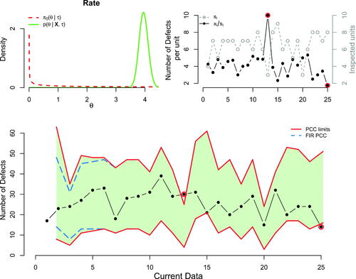
Table 7. Number of defects (x_i) and inspected units (s_i) per time point ($i=1,2,\dots ,25$), in an assembly line of an electrical equipment.

Inspected units $(s_1-s_{13})$	4	7	5	7	7	7	6	7	7	6	8	6	3
Defect counts $(x_1-x_{13})$	17	23	24	27	32	33	18	28	29	31	39	29	30
Inspected units $(s_{14}-s_{25})$	8	9	6	7	5	7	3	6	8	8	7	8
Defect counts $(x_{14}-x_{25})$	31	21	26	20	24	29	15	32	20	24	24	14

7. Conclusions

In this work we proposed a new general Bayesian method that permits online process monitoring for various types of data, as long as their distribution belongs to the regular exponential family. The use of initial and/or power prior distribution, offers an axiomatic framework where subjective knowledge and/or historical data can be incorporated in the decision making scheme allowing valid online inference, from the very early start of the process, aborting the need of phase I. It is the use of prior distribution that provides a structural advantage over the non-parametric and self-starting frequentist based methods, especially in shorts runs and phase I data, where only brief IC information is available from the current data. The effect of the prior settings (as long as we avoid extremely informative priors), will decay soon, as more data become available. Furthermore, for users that might not be accustomed to the Bayesian approach, the choice of non-informative (reference or Jeffeys) prior, allows direct PCC implementation, using only the incoming data (and historical data if available).

PCC emphasizes in online outlier detection of short production runs and it does not require a phase I/II split. Traditional phase I studies, where online inference regarding the presence of large transient shifts is of interest, are ideal settings for PCC. Furthermore, it is feasible for a user to switch from standard phase I/II monitoring methods to PCC, as it will not only provide online outlier detection monitoring during the “phase I” segment, but thanks to its sequentially updated nature, it will allow incorporation of the “phase II” data into the monitoring mechanism (something that is not done with typical frequentist methods). Thanks to the Bayesian posterior distribution, we are also able to perform inference regarding each of the unknown parameters.

PCC seems to be ideal for everyone that deals with either short runs or applications that require online monitoring during phase I. However, practitioners that employ a traditional phase I/II protocol in their routine, can benefit from the use of PCC during their phase I. Precisely, they will not only be able to monitor the process online while in phase I, but also obtain the posterior point estimates of the unknown parameters at the end of phase I, that will be necessary to build traditional phase II control charts. The benefits are significant in short runs, where most of the existing methods are unable to have robust performance and reliable estimates of the unknown parameter(s).

Acknowledgments

We are grateful to the editor and the two anonymous referees, whose valuable comments and suggestions improved significantly the manuscript. We would also like to thank Frederic Sobas from Hospices Civils de Lyon, who provided the data set used in the Normal PCC, but more importantly for his invaluable feedback from using the suggested PCC at the daily Internal Quality Control routine in the medical labs of Hospices Civils de Lyon. This research was partially funded by the Research Center of the Athens University of Economics and Business.

Additional information

Funding

Research Center, Athens University of Economics and Business.

Notes on contributors

Konstantinos Bourazas

Konstantinos Bourazas is currently a Ph.D. candidate in the department of Statistics at the Athens University of Economics and Business, Greece. His research interest is mainly focused on Bayesian statistical process control and monitoring and sequential change point models with applications in the bio-medical area.

Dimitrios Kiagias

Dimitrios Kiagias is currently a Research Associate in the School of Mathematics and Statistics at the University of Sheffield. His main research areas are on Bayesian methodologies and applications on quality control schemes, clinical trials and image analysis of biological systems. His email is: [email protected].

Panagiotis Tsiamyrtzis

Panagiotis Tsiamyrtzis is currently an Associate Professor at the Department of Mechanical Engineering, Politecnico di Milano and his email is [email protected].

Appendix A.

Proof of Theorem 1

For a likelihood $f(·|\mathit{\theta }),$ being a member of the k-PREF, the conjugate prior is (Bernardo and Smith 2000): $${\pi }_0\left(\mathit{\theta }|\mathit{\tau }\right)={\left[K(\mathit{\tau })\right]}^{-1}{[c(\mathit{\theta })]}^{{\tau }_0}\hspace{0.17em}\text{exp}\hspace{0.17em}\left\{\sum _{i=1}^k{\eta }_i(\mathit{\theta }){\tau }_i\right\},$$ where $\mathit{\tau }=({\tau }_0,{\tau }_1,\dots ,{\tau }_k)$ is the $(k+1)$-dimensional vector of the initial prior hyperparameters, such that for the normalizing constant, $K(\mathit{\tau }),$ it holds: $$K(\mathbf{\tau })=\underset{\mathbf{\Theta }}{\int }{[c(\mathbf{\theta })]}^{{\tau }_0}\hspace{0.17em}\text{exp}\hspace{0.17em}\left\{\sum _{i=1}^k{\eta }_i(\mathbf{\theta }){\tau }_i\right\}d\mathbf{\theta }<\infty ,$$ (for discrete $\mathit{\theta },$ we replace the integral sign by summation). Then for the historical data $\mathit{Y}=(y_1,\dots ,y_{n_0}),$ sampled from the same member of the k-PREF as the likelihood, $f(·|\mathit{\theta }),$ the power prior will become: $$\begin{array}{c}\pi \left(\mathit{\theta }|\mathit{Y},{\alpha }_0,\mathit{\tau }\right)\propto f{\left(\mathit{Y}|\mathit{\theta }\right)}^{{\alpha }_0}{\pi }_0\left(\mathit{\theta }|\mathit{\tau }\right)\\ ={\left[\prod _{l=1}^{n_0}g(y_l)\right]}^{{\alpha }_0}{[c(\mathit{\theta })]}^{{\alpha }_0{n}_0}\hspace{0.17em}\text{exp}\hspace{0.17em}\left\{{\alpha }_0\sum _{i=1}^k{\eta }_i(\mathit{\theta })\sum _{l=1}^{n_0}{h}_i(y_l)\right\}\times \\ \times {[K(\mathit{\tau })]}^{-1}{[c(\mathit{\theta })]}^{{\tau }_0}\hspace{0.17em}\text{exp}\hspace{0.17em}\left\{\sum _{i=1}^k{\eta }_i(\mathit{\theta }){\tau }_i\right\}\\ ={[K(\mathit{\tau })]}^{-1}{\left[\prod _{l=1}^{n_0}g(y_l)\right]}^{{\alpha }_0}{[c(\mathit{\theta })]}^{{\tau }_0+{\alpha }_0{n}_0}\hspace{0.17em}\text{exp}\hspace{0.17em}\left\{\sum _{i=1}^k{\eta }_i(\mathit{\theta })\left({\tau }_i+{\alpha }_0\sum _{l=1}^{n_0}{h}_i(y_l)\right)\right\}\\ \propto {[c(\mathit{\theta })]}^{{\tau }_0+{\alpha }_0{n}_0}\hspace{0.17em}\text{exp}\hspace{0.17em}\left\{\sum _{i=1}^k{\eta }_i(\mathit{\theta })\left({\tau }_i+{\alpha }_0\sum _{l=1}^{n_0}{h}_i(y_l)\right)\right\}\\ \propto {\pi }_0\left(\mathit{\theta }|\mathit{\tau }+{\alpha }_0{\mathit{t}}_{n_0}(\mathit{Y})\right),\end{array}$$ where ${\mathit{t}}_{n_0}(\mathit{Y})=(n_0,{\sum }_{l=1}^{n_0}{h}_1(y_l),\dots ,{\sum }_{l=1}^{n_0}{h}_k(y_l))$ is a $(k+1)$-dimensional vector, with $\mathit{Y}=(y_1,\dots ,y_{n_0})$ referring to the vector of historical data. Then once the current data $\mathit{X}=(x_1,\dots ,x_n)$ become available, we will be able to derive the posterior distribution of the unknown parameter(s) $\mathit{\theta },$ using Bayes theorem: $$\begin{array}{c}p\left(\mathit{\theta }|\mathit{X},\mathit{Y},{\alpha }_0,\mathit{\tau }\right)\propto f\left(\mathit{X}|\mathit{\theta }\right)\pi \left(\mathit{\theta }|\mathit{Y},{\alpha }_0,\mathit{\tau }\right)\\ \propto f\left(\mathit{X}|\mathit{\theta }\right){\pi }_0\left(\mathit{\theta }|\mathit{\tau }+{\alpha }_0{\mathit{t}}_{n_0}(\mathit{Y})\right)\\ =\left[\prod _{j=1}^{n}g(x_j)\right]{[c(\mathit{\theta })]}^n\hspace{0.17em}\text{exp}\hspace{0.17em}\left\{\sum _{i=1}^k{\eta }_i(\mathit{\theta })\sum _{j=1}^n{h}_i(x_j)\right\}\times \\ \times {[K(\mathit{\tau })]}^{-1}{\left[\prod _{l=1}^{n_0}g(y_l)\right]}^{{\alpha }_0}{[c(\mathit{\theta })]}^{{\tau }_0+{\alpha }_0{n}_0}\hspace{0.17em}\text{exp}\hspace{0.17em}\left\{\sum _{i=1}^k{\eta }_i(\mathit{\theta })\left({\tau }_i+a_0\sum _{l=1}^{n_0}{h}_i(y_l)\right)\right\}\\ \propto {[c(\mathit{\theta })]}^{{\tau }_0+{\alpha }_0{n}_0+n}\hspace{0.17em}\text{exp}\hspace{0.17em}\left\{\sum _{i=1}^k{\eta }_i(\mathit{\theta })\left({\tau }_i+a_0\sum _{l=1}^{n_0}{h}_i(y_l)+\sum _{j=1}^n{h}_i(x_j)\right)\right\}\\ \propto {\pi }_0\left(\mathit{\theta }|\mathit{\tau }+{\alpha }_0{\mathit{t}}_{n_0}(\mathit{Y})+{\mathit{t}}_n(\mathit{X})\right),\end{array}$$ where ${\mathit{t}}_n(\mathit{X})=(n,{\sum }_{j=1}^n{h}_1(x_j),\dots ,{\sum }_{j=1}^n{h}_k(x_j))$ is a $(k+1)$-dimensional vector, with $\mathit{X}=(x_1,\dots ,x_n)$ being the observed data. This is a member of exponential family, and specifically of the same distribution form as the initial prior (as expected since we use a conjugate prior).

For (ii) we have that the predictive distribution of a future observable will be given by: $f(X_{n+1}|\mathit{X},\mathit{Y},{\alpha }_0,\mathit{\tau })=$ $$\begin{array}{c}=\underset{\mathbf{\Theta }}{\int }f\left(X_{n+1}|\mathit{\theta }\right)p\left(\mathit{\theta }|\mathit{X},\mathit{Y},{\alpha }_0,\mathit{\tau }\right)d\mathit{\theta }\\ =\underset{\mathbf{\Theta }}{\int }\left[g(X_{n+1})c(\mathit{\theta })\hspace{0.17em}\text{exp}\hspace{0.17em}\left\{\sum _{i=1}^k{\eta }_i(\mathit{\theta })h_i(X_{n+1})\right\}\right]\times [{\left[K\left(\mathit{\tau }+{\alpha }_0{\mathit{t}}_{n_0}(\mathit{Y})+{\mathit{t}}_n(\mathit{X})\right)\right]}^{-1}\\ {[c(\mathit{\theta })]}^{{\tau }_0+{\alpha }_0{n}_0+n}\hspace{0.17em}\text{exp}\hspace{0.17em}\left\{\sum _{i=1}^k{\eta }_i(\mathit{\theta })\left({\tau }_i+a_0\sum _{l=1}^{n_0}{h}_i(y_l)+\sum _{j=1}^n{h}_i(x_j)\right)\right\}]d\mathit{\theta }\\ ={\left[K\left(\mathit{\tau }+{\alpha }_0{\mathit{t}}_{n_0}(\mathit{Y})+{\mathit{t}}_n(\mathit{X})\right)\right]}^{-1}g(X_{n+1})\times \\ \underset{\mathbf{\Theta }}{\int }{\left[c(\mathit{\theta })\right]}^{{\tau }_0+{\alpha }_0{n}_0+n+1}\hspace{0.17em}\text{exp}\hspace{0.17em}\left\{\sum _{i=1}^k{\eta }_i(\mathit{\theta })\left({\tau }_i+a_0\sum _{l=1}^{n_0}{h}_i(y_l)+\sum _{j=1}^n{h}_i(x_j)+h_i(X_{n+1})\right)\right\}d\mathit{\theta }\Rightarrow \\ f\left(X_{n+1}|\mathit{X},\mathit{Y},{\alpha }_0,\mathit{\tau }\right)=\frac{K\left(\mathit{\tau }+{\alpha }_0{\mathit{t}}_{n_0}(\mathit{Y})+{\mathit{t}}_n(\mathit{X})+{\mathit{t}}_1(X_{n+1})\right)}{K\left(\mathit{\tau }+{\alpha }_0{\mathit{t}}_{n_0}(\mathit{Y})+{\mathit{t}}_n(\mathit{X})\right)}g(X_{n+1}),\end{array}$$ where ${\mathit{t}}_1(X_{n+1})=(1,h_1(X_{n+1}),\dots ,h_k(X_{n+1}))$ a $(k+1)$-dimensional vector, function of the future observable $X_{n+1}.$ Note that the vectors ${\mathit{t}}_{n_0}(\mathit{Y}),{\mathit{t}}_n(\mathit{X})$ and ${\mathit{t}}_1(X_{n+1})$ refer to the respective sufficient statistics for the power prior and the likelihood.

Q.E.D.

Appendix B.

On HPrD regions

We provide the definition of Highest Predictive Density (HPrD), which is used for the sequential tests of PCC. Assume the set R^c which contains the values of the predictive density (or mass) function, which are greater than a threshold c, i.e.: (B1) $$R^c=\{x_{n+1}:f(x_{n+1}|\mathit{D},\mathit{w},\mathit{\tau })\ge c\}.$$(B1)

The HPrD region will be given by minimizing the absolute difference of a highest predictive probability from a significance level $1-a,$ for all the possible values of c. Specifically: (B2) $$R_{n+1}={\underset{R^c}{\min }}_{}\left|\underset{R^c}{\int }f(x_{n+1}|\mathit{D},\mathit{w},\mathit{\tau })-(1-a)\right|,$$(B2) for the discrete case, we replace the integral sign by summation. $R_{n+1}$ will be the shortest region with the smallest absolute difference from the probability $1-a.$ In other words, it minimizes the Lebesque measure $m(R^c)$ for continuous cases or the corresponding measure $l(R^c)={\sum }_i{\delta }_{x_i}(f(x_i|\mathit{D},\mathit{w},\mathit{\tau })\ge c)$ for discrete cases, where ${\delta }_{x_i}(·)$ represents the Dirac delta function.

For continuous distributions the HPrD region is calculated just like the Highest Posterior Density (HPD) region in Bayesian analysis (see for example Carlin and Louis 2009), where instead of the posterior, we use the predictive distribution and the minimum value of the absolute difference will be 0. For discrete predictive distributions, typically we will not be able to obtain a region that has the exact coverage probability $1-\alpha .$ In this case the HPrD can be obtained by starting from the mode of the predictive distribution and continue adding sequentially the next most probable values of the predictive distribution, until we get sufficiently close (minimizing the absolute difference) to the predetermined coverage level $1-\alpha .$ Algorithm 1 provides the details in how to derive the HPrD region for a discrete predictive distribution and Figure B1 provides an illustration.

Figure B1. The HPrD region $(R_{n+1})$ for continuous (left panel) and discrete (right panel) data.

Algorithm 1. HPrD algorithm for a discrete distribution

1: Set p_i the i^th decreasing ordered probability of $f(X_{n+1}|\mathit{X},\mathit{Y},{\alpha }_0,\mathit{\tau }),$ e.g., p₁ is the $\max$

2: Set $z_i=\arg \left\{p_i\right\},$ i.e., the argument(s) where p_i get their values

3:$n\leftarrow 1$ ⊳ initial values

4: $\mathit{sum}\_\mathit{probs}\leftarrow 0$

5:$\mathit{diff}\leftarrow 1$

6:$\mathit{HPrD}\leftarrow \varnothing$

7:$\mathit{stop}\leftarrow 0$

8: while stop = 0

9: $\mathit{sum}\_\mathit{probs}\leftarrow \mathit{sum}\_\mathit{probs}+p_n$

10: if $\left|\mathit{sum}\_\mathit{probs}-(1-a)\right|<\mathit{diff}$

11:  $\mathit{HPrD}\leftarrow \{\mathit{HPrD},z_n\}$

12:  $\mathit{diff}\leftarrow \left|\mathit{sum}\_\mathit{probs}-(1-a)\right|$

13:  $n\leftarrow n+1$

14: else

15:  $\mathit{stop}\leftarrow 1$

16: $\mathit{HPrD}\leftarrow \mathit{sort}\left\{\mathit{HPrD}\right\}$

We should also note here that in symmetric discrete predictive distributions (like a Beta Binomial with $\alpha =\beta$), the HPrD region might not be unique, as there might exist two regions that achieve the minimum of absolute difference (we can choose at random).

Appendix C.

PCC algorithm

Algorithm 2. PCC algorithm

1: Select the significance level α, based on FWER or ARL₀⊳ FAR

2: Choose the data distribution and the conjugate prior density for $\mathit{\theta }$⊳ distributions

3: Is FIR-PCC of interest?⊳ FIR

4: YES

5: Determine the parameters f and $\mathrm{a}$

6: NO

7: Set f = 1

8: Is prior information available?⊳ initial prior ${\pi }_0(·)$

9: YES

10: Determine the hyperparameters of the initial prior $\mathit{\tau }$

11: NO

12: Set the initial reference/Jeffeys prior (see Table E1, Appendix E)

Table E1. Initial Reference (R) and Jeffreys (J) prior distributions.

Likelihood	Initial Reference/Jeffreys Prior
$f(·|\mathit{\theta })$	${\pi }_0(\mathit{\theta }|\mathit{\tau })$
P$(\theta ·s_i)$	${\pi }_0(\theta )\propto \frac{1}{\sqrt{\theta }}\equiv G(1/2,0)$
Bin$(N_i,\theta )$	${\pi }_0(\theta )\propto \frac{1}{\sqrt{\theta (1-\theta )}}\equiv \mathit{Beta}(1/2,1/2)$
NBin$(r,\theta )$	${\pi }_0(\theta )\propto \frac{1}{\theta \sqrt{(1-\theta )}}\equiv \mathit{Beta}(0,1/2)$
W$(\theta ,\kappa )$	${\pi }_0({\theta }^{\kappa })\propto \frac{1}{{\theta }^{\kappa }}\equiv IG(0,0)$
G$(a,\theta ),$ IG$(a,\theta ),$ Pa$(m,\theta )$	${\pi }_0(\theta )\propto \frac{1}{\theta }\equiv G(0,0)$
N$(\theta ,{\sigma }^2),$ LogN$(\theta ,{\sigma }^2)$	${\pi }_0(\theta )\propto c\equiv N(0,+\infty )$
N$(\mu ,{\theta }^2),$ LogN$(\mu ,{\theta }^2)$	${\pi }_0({\theta }^2)\propto \frac{1}{{\theta }^2}\equiv IG(0,0)$
N$({\theta }_1,{\theta }_2^2),$ LogN$({\theta }_1,{\theta }_2^2)$	${\pi }_0^R({\theta }_1,{\theta }_2^2)\propto \frac{1}{{\theta }_2^2}\equiv \mathit{NIG}(0,0,-1/2,0),{\pi }_0^J({\theta }_1,{\theta }_2^2)\propto \frac{1}{{\theta }_2^3}\equiv \mathit{NIG}(0,0,0,0)$

For univariate $\mathit{\theta }$ the two classes of non-informative priors coincide.

13: Are prior data available?⊳ power prior

14: YES

15: Provide the historical data Y and determine ${\alpha }_0$

16: NO

17: Set ${\alpha }_0=0$

18: Once the data point x_n ($n\ge 1^{★}$) arrives, derive the predictive distribution of next observable $X_{n+1}|(\mathit{X},\mathit{Y},{\alpha }_0,\mathit{\tau })$

19: Derive the $FI{R}_{\mathit{adj}}·100(1-\alpha )\%$ HPrD region, obtain $x_{n+1}$ and draw it⊳ $R_{n+1}$

20: if $x_{n+1}\in R_{n+1}$⊳ test

21: $n\leftarrow n+1$

22: goto 18

23: else⊳ alarm!

24: if you do not make a corrective action

25:  then goto 21

26: else

27: end

${}^{★}$ For the Normal – NIG model using the initial reference prior and ${\alpha }_0=0$ we need n = 2 to initiate PCC, while for all other cases PCC starts at after x₁ becomes available.

Appendix D.

Proof of Lemma 2

Following Quesenberry (1991a) the Q-chart in all three cases of the Normal distribution, makes use at each data point $x_{n+1},$ of the statistic $Q_{n+1}.$ For PCC we set ${\alpha }_0=0,$ eliminating the power prior part regarding the past data (Y) and in each case we set the hyperparameters $\mathit{\tau },$ so that we have the respective reference prior for the unknown parameter(s). We will show that controlling $Q_{n+1}$ statistic is identical to controlling PCC’s standardized predictive residual: $$P{R}_{n+1}=\frac{X_{n+1}-{\widehat{\mu }}_n}{{\widehat{\sigma }}_n}$$ where, ${\widehat{\mu }}_n$ and ${\widehat{\sigma }}_n$ are the mean and standard deviation respectively of the predictive distribution of $X_{n+1}|(\mathit{X},\mathit{Y},{\alpha }_0=0,\mathit{\tau })\equiv X_{n+1}|(\mathit{X},\mathit{\tau }).$ Denoting by ${\Phi }^{-1}(·)$ the inverse of the standard normal CDF and $G_{\nu }(·)$ the Student-t CDF with ν degrees of freedom we get:

Case I: μ unknown, ${\sigma }^2$ known.

We have: $X_i|\theta \sim N(\theta ,{\sigma }^2)$ and the reference prior is $\pi (\theta )\propto c\equiv N(0,+\infty ).$ Then the predictive distribution will be: $$X_{n+1}|\left(\mathit{X},\mathit{\tau }\right)\sim N\left({\overline{x}}_n,\frac{n+1}{n}{\sigma }^2\right)\Rightarrow P{R}_{n+1}=\frac{X_{n+1}-{\overline{x}}_n}{\sqrt{\frac{n+1}{n}}\sigma }=Q_{n+1}\sim N(0,1).$$

Case II: μ known, ${\sigma }^2$ unknown.

We have: $X_i|\theta \sim N(\mu ,{\theta }^2)$ and the reference prior is $\pi ({\theta }^2)\propto 1/{\theta }^2\equiv IG(0,0).$ Then the predictive distribution will be: $$X_{n+1}|\left(\mathit{X},\mathit{\tau }\right)\sim t_{n-1}\left(\mu ,\frac{\sum _{j=1}^n{\left(x_j-\mu \right)}^2}{n}\right)\Rightarrow P{R}_{n+1}=\frac{X_{n+1}-\mu }{\sqrt{\frac{\sum _{j=1}^n{\left(x_j-\mu \right)}^2}{n}}}\sim t_{n-1}.$$

Transformating the $P{R}_{n+1}$ we get: ${\Phi }^{-1}\left\{G_{n-1}(P{R}_{n+1})\right\}=Q_{n+1}\sim N(0,1).$

Case III: μ unknown and ${\sigma }^2$ unknown.

We have: $X_i|\theta \sim N({\theta }_1,{\theta }_2^2)$ and the reference prior is $\pi ({\theta }_1,{\theta }_2^2)\propto 1/{\theta }_2^2\equiv \mathit{NIG}(0,0,-1/2,0).$ Then the predictive distribution will be: $$X_{n+1}|\left(\mathit{X},\mathit{\tau }\right)\sim t_{n-2}\left({\overline{x}}_n,\frac{\sum _{j=1}^n{\left(x_j-{\overline{x}}_n\right)}^2}{n-1}\right)\Rightarrow P{R}_{n+1}=\frac{X_{n+1}-{\overline{x}}_n}{\sqrt{\frac{\sum _{j=1}^n{\left(x_j-{\overline{x}}_n\right)}^2}{n-1}}}\sim t_{n-2}.$$

Transformating again the $P{R}_{n+1}$ we get: ${\Phi }^{-1}\left\{G_{n-2}(P{R}_{n+1})\right\}=Q_{n+1}\sim N(0,1).$

For cases II and III, as the functions ${\Phi }^{-1}(·)$ and $G_{\nu }(·)$ are injective, it is identical to control $P{R}_{n+1}$ or $Q_{n+1}.$

Q.E.D.

Appendix E.

Guidelines regarding the initial prior ${\mathit{\pi }}_{\mathit{0}}(\mathit{\theta }|\mathit{\tau })$ elicitation

The big advantage of PCC is the use of typically available prior information, which allows to decrease the uncertainty of the unknown parameter(s) $\mathit{\theta },$ improving the performance (with respect to false alarms and detection power), especially at the early stages. The speed at which this uncertainty decreases is inversely related to the information that the prior distribution carries. When strong opinion about the unknown parameter(s) is available and located accurately (i.e., we have highly informative initial prior placed at the parameter space where the unknown parameter is), then the PCC performance will be optimal (FWER at the nominal level and quite high detection power). Nevertheless, a highly informative prior miss-placed on the parameter space (with respect to where the true unknown $\mathit{\theta }$ is), will have as result to get an extremely high FAR (until sufficient information from the data moves the posterior to the area where the true $\mathit{\theta }$ lies). Thus, a general recommendation is to avoid having a highly informative initial prior distribution (to eliminate the risk of inflated false alarms if miss-placed). Wang et al. (2018) developed effective numerical methods for exploring reasonable choices of an informative prior distribution.

From the above it becomes evident that the elicitation of the hyper-parameters $\mathit{\tau }$ play an important role to PCC. There are two different ways that one can proceed: being subjective or objective. In the latter we use non-informative priors and in a sense we leave the data to carry the information. In the former we use a low/medium (but not high) informative prior distribution. Such a prior will carry more information compared to the objective priors (reducing the posterior variability of $\mathit{\theta }$) enhancing the PCC performance, especially at the start of the process. Furthermore, as the size of the data increases, the influence of the low/medium information prior is washing-out.

In the case where no prior information for $\mathit{\theta }$ exists, or a user prefers to follow an objective prior approach, then the hyper-parameters determination should be chosen with caution, especially when we do not have historical data to use in a power prior (i.e., ${\alpha }_0=0$). Various classes of non-informative priors exist like:

• Flat prior: a uniform prior equally weighting all possible values of the unknown parameter.

• Jeffreys prior: a prior that is closed under parameter transformations.

• Reference prior: a function that maximizes some measure of distance (e.g., Hellinger) or divergence (e.g., Kullback-Leibler) between the posterior and prior, as data become available.

A list of Jeffreys and reference initial priors that can be used for likelihoods that are members of the k-PREF are given in Table E1. When we need to choose an “objective” prior we should aim to satisfy the following properties: have the minimal possible influence in the process, do not decrease the reflexes of PCC and attempt to have stable false alarm performance. Based on this proposal we will next provide more specific details along with some guidelines for the likelihoods that studied in the simulation study (i.e., Normal, Poisson, and Binomial).

For the $N({\theta }_1,{\theta }_2^2)-\mathit{NIG}({\mu }_0,\lambda ,a,b)$ model, we have to carefully determine the parameters of the Inverse Gamma (i.e., a and b). For example, the prior $\mathit{NIG}(0,ϵ,ϵ,ϵ)$ (which converges to Jeffreys prior as $ϵ\to 0$) gives higher density at values of ${\theta }_2^2$ which are close to 0. Thus, it becomes very informative, increasing drastically the false alarms especially for large values of ${\theta }_2^2.$ Similar results hold for $\mathit{NIG}(0,ϵ,1/2,ϵ)$ and $\mathit{NIG}(0,ϵ,1,ϵ),$ where the mean of the marginal posterior of ${\theta }_2^2$ is the MLE and the unbiased estimator respectively. On the other hand, a flatter prior like $\mathit{NIG}(0,ϵ,ϵ,1)$ may overestimate ${\theta }_2^2$ reducing the reflexes of PCC. Generally, we recommend to choose a value for the hyper-parameter a > 2, so that the mean and the variance of the prior Inverse Gamma is defined. In different cases, the prior parameters have to be determined carefully.

For the $P({\theta }_3)-\mathit{Gamma}(c,d)$ model, the initial prior $\mathit{Gamma}(ϵ,ϵ)$ seems not to be a good choice. Despite that the posterior mean is the MLE, this prior may increase the number of false alarms, especially when θ₃ is close to 0. In that case, if x_n = 0, then the HPrD region $R_{n+1}$ will shrink to a short region. In general we found that small values for both of the hyper-parameters c and d (e.g., less than 1/3) tend to affect $R_{n+1}$ in the same manner, even when the prior mean is correctly located.

For $\mathit{Bin}(N,{\theta }_4)-\mathit{Beta}(a,b)$ model we propose to avoid $\mathit{Beta}(ϵ,ϵ),$ which converges to Haldane’s prior (Haldane 1932) as $ϵ\to 0,$ where the posterior mean is equal to the MLE, as we will have inflated false alarms. Also, choosing small values for both of the hyper-parameters a and b (e.g., less than 1/3), especially if θ₄ is close to 0 as we will have inflated false alarms (just as we had in the Poisson-Gamma respective case). In contrary, the flat Beta(1, 1), equally weighting all values of θ₄, will have the posterior mode to be the MLE and provide weak information, inflating the predictive. Thus, the detection performance of PCC will be affected.

Generally, reference priors (Bernardo 1979) and Neutral priors (Kerman 2011) provide a stable start to PCC under a total prior ignorance. Our proposal though, when some information about the unknown parameters exists, is to adopt a medium/low volume information prior ${\pi }_0(\mathit{\theta }|\mathit{\tau })$ which will enhance the PCC performance (compared to non-informative choices) and its effect will be removed once a short sequence of data becomes available.

References

- Ali, S. 2020. A predictive Bayesian approach to sequential time-between-events monitoring. Quality and Reliability Engineering International 36 (1):365–87. doi: 10.1002/qre.2580.
- Apley, D. W. 2012. Posterior distribution charts: A Bayesian approach for graphically exploring a process mean. Technometrics 54 (3):279–310. doi: 10.1080/00401706.2012.694722.
- Atalay, M., M. Caner Testik, S. Duran, and C. H. Weiß. 2020. Guidelines for automating phase I of control charts by considering effects on phase-II performance of individuals control chart. Quality Engineering 32 (2):223–43. doi:10.1080/08982112.2019.1641208
- Bayarri, M. J., and G. García-Donato. 2005. A Bayesian sequential look at u-control charts. Technometrics 47 (2):142–51. doi: 10.1198/004017005000000085.
- Berger, J. O., J. M. Bernardo, and D. Sun. 2009. The formal definition of reference priors. Annals of Statistics 37:905–38.
- Bernardo, J. M. 1979. Reference posterior distributions for Bayesian inference. Journal of the Royal Statistical Society: Series B (Methodological) 41 (2):113–47. doi: 10.1111/j.2517-6161.1979.tb01066.x.
- Bernardo, J. M., and A. F. M. Smith. 2000. Bayesian theory. 1st ed. New York: Wiley.
- Capizzi, G., and G. Masarotto. 2013. Phase I distribution-free analysis of univariate data. Journal of Quality Technology 45 (3):273–84. doi: 10.1080/00224065.2013.11917938.
- Capizzi, G., and G. Masarotto. 2020. Guaranteed in-control control chart performance with cautious parameter learning. Journal of Quality Technology 52 (4):385–403. doi:10.1080/00224065.2019.1640096
- Carlin, B. P., and T. A. Louis. 2009. Bayesian methods for data analysis. London: Chapman & Hall.
- Chakraborti, S., S. W. Human, and M. A. Graham. 2008. Phase I statistical process control charts: An overview and some results. Quality Engineering 21 (1):52–62. doi: 10.1080/08982110802445561.
- Dasdemir, E., C. Weiß, M. C. Testik, and S. Knoth. 2016. Evaluation of phase I analysis scenarios on phase II performance of control charts for autocorrelated observations. Quality Engineering 28 (3):293–304. doi: 10.1080/08982112.2015.1104540.
- Deming, W. E. 1986. Out of crisis. Cambridge, MA: The MIT Press.
- Dunn, O. J. 1961. Multiple comparisons among means. Journal of the American Statistical Association 56 (293):52–64. doi: 10.1080/01621459.1961.10482090.
- Geisser, S. 1993. Predictive inference: An introduction. London: Chapman & Hall.
- Goedhart, R., M. Schoonhoven, and R. J. Does. 2017. Guaranteed in-control performance for the Shewhart X and X¯ control charts. Journal of Quality Technology 49 (2):155–71.
- Haldane, J. B. S. 1932. A note on inverse probability. Mathematical Proceedings of the Cambridge Philosophical Society 28 (1):55–61. doi: 10.1017/S0305004100010495.
- Hansen, B., and P. Ghare. 1987. Quality control and application. Englewood Cliffs, NJ: Prentice-Hall.
- Hawkins, D. M., and D. H. Olwell. 1998. Cumulative sum charts and charting for quality improvement. New York: Springer.
- Ibrahim, J., and M. Chen. 2000. Power prior distributions for regression models. Statistical Science 15:46–60.
- Ibrahim, J., M. Chen, and D. Sinha. 2003. On optimality properties of the power prior. Journal of the American Statistical Association 98 (461):204–13. doi: 10.1198/016214503388619229.
- Jeffreys, H. 1961. Theory of probability. 3rd ed. Oxford: Oxford University Press.
- Jensen, W. A., L. A. Jones-Farmer, C. W. Champ, and W. H. Woodall. 2006. Effects of parameter estimation on control chart properties: A literature review. Journal of Quality Technology 38 (4):349–64. doi: 10.1080/00224065.2006.11918623.
- Jones-Farmer, L. A., W. H. Woodall, S. H. Steiner, and C. W. Champ. 2014. An overview of phase I analysis for process improvement and monitoring. Journal of Quality Technology 46 (3):265–80. doi: 10.1080/00224065.2014.11917969.
- Kadoishi, S., and H. Kawamura. 2020. Control charts based on hierarchical Bayesian modeling. Total Quality Science 5 (2):72–80. doi: 10.17929/tqs.5.72.
- Keefe, M. J., W. H. Woodall, and L. A. Jones-Farmer. 2015. The conditional in-control performance of self-starting control charts. Quality Engineering 27 (4):488–99. doi: 10.1080/08982112.2015.1065323.
- Kerman, J. 2011. Neutral noninformative and informative conjugate beta and gamma prior distributions. Electronic Journal of Statistics 5:1450–70. doi: 10.1214/11-EJS648.
- Kumar, N., and S. Chakraborti. 2017. Bayesian monitoring of times between events: The Shewhart tr-chart. Journal of Quality Technology 49 (2):136–54. doi: 10.1080/00224065.2017.11917985.
- Lee, J., N. Wang, L. Xu, A. Schuh, and W. H. Woodall. 2013. The effect of parameter estimation on upper-sided Bernoulli cumulative sum charts. Quality and Reliability Engineering International 29 (5):639–51. doi: 10.1002/qre.1413.
- Lucas, J. M., and R. B. Crosier. 1982. Fast initial response for CUSUM quality-control schemes: Give your CUSUM a head start. Technometrics 24 (3):199–205. doi: 10.1080/00401706.1982.10487759.
- Madrid Padilla, O. H., A. Athey, A. Reinhart, and J. G. Scott. 2019. Sequential nonparametric tests for a change in distribution: An application to detecting radiological anomalies. Journal of the American Statistical Association 114 (526):514–28. doi: 10.1080/01621459.2018.1476245.
- Menzefricke, U. 2002. On the evaluation of control chart limits based on predictive distributions. Communications in Statistics - Theory and Methods 31 (8):1423–40. doi: 10.1081/STA-120006077.
- Montgomery, D. C. 2009. Introduction to statistical quality control. 6th ed. New York: Wiley.
- Qiu, P. 2014. Introduction to statistical process control. London: CRC Press, Chapman & Hall.
- Quesenberry, C. P. 1991a. SPC Q charts for start-up processes and short or long runs. Journal of Quality Technology 23 (3):213–24. doi: 10.1080/00224065.1991.11979327.
- Quesenberry, C. P. 1991b. SPC Q charts for a binomial parameter p: Short or long runs. Journal of Quality Technology 23 (3):239–46. doi: 10.1080/00224065.1991.11979329.
- Quesenberry, C. P. 1991c. SPC Q charts for a Poisson parameter: Short or long runs. Journal of Quality Technology 23 (4):296–303. doi: 10.1080/00224065.1991.11979345.
- Shen, X., K. L. Tsui, C. Zou, and W. H. Woodall. 2016. Self-starting monitoring scheme for Poisson count data with varying population sizes. Technometrics 58 (4):460–71. doi: 10.1080/00401706.2015.1075423.
- Šidák, Z. K. 1967. Rectangular confidence regions for the means of multivariate normal distributions. Journal of the American Statistical Association 62 (318):626–33. doi: 10.1080/01621459.1967.10482935.
- Steiner, S. H. 1999. EWMA control charts with time-varying control limits and fast initial response. Journal of Quality Technology 31 (1):75–86. doi: 10.1080/00224065.1999.11979899.
- Tsiamyrtzis, P., and D. M. Hawkins. 2005. A Bayesian scheme to detect changes in the mean of a short run process. Technometrics 47 (4):446–56. doi: 10.1198/004017005000000346.
- Tsiamyrtzis, P., and D. M. Hawkins. 2010. Bayesian start up phase mean monitoring of an autocorrelated process that is subject to random sized jumps. Technometrics 52 (4) :438–52. doi: 10.1198/TECH.2010.08053.
- Tsiamyrtzis, P., and D. M. Hawkins. 2019. Statistical process control for phase I count type data. Applied Stochastic Models in Business and Industry 35 (3):766–87. doi: 10.1002/asmb.2398.
- Wang, X., D. J. Nott, C. C. Drovandi, K. Mengersen, and M. Evans. 2018. Using history matching for prior choice. Technometrics 60 (4):445–60. doi: 10.1080/00401706.2017.1421587.
- Woodward, P. W., and J. C. Naylor. 1993. An application of Bayesian methods in SPC. The Statistician 42 (4):461–9. doi: 10.2307/2348478.
- Zhang, M., F. M. Megahed, and W. H. Woodall. 2014. Exponential CUSUM charts with estimated control limits. Quality and Reliability Engineering International 30 (2):275–86. doi: 10.1002/qre.1495.
- Zhang, M., Y. Peng, A. Schuh, F. M. Megahed, and W. H. Woodall. 2013. Geometric charts with estimated control limits. Quality and Reliability Engineering International 29 (2):209–23. doi: 10.1002/qre.1304.
- Zellner, A. 1988. Optimal information processing and Bayes’s theorem. The American Statistician 42 (4):278–80.