Predictive ratio CUSUM (PRC): A Bayesian approach in online change point detection of short runs

Abstract

The online quality monitoring of a process with low volume data is a very challenging task and the attention is most often placed in detecting when some of the underline (unknown) process parameter(s) experience a persistent shift. Self-starting methods, both in the frequentist and the Bayesian domain aim to offer a solution. Adopting the latter perspective, we propose a general closed-form Bayesian scheme, where the testing procedure is built on a memory-based control chart that relies on the cumulative ratios of sequentially updated predictive distributions. The theoretic framework can accommodate any likelihood from the regular exponential family and the use of conjugate analysis allows closed form modeling. Power priors will offer the axiomatic framework to incorporate into the model different sources of information, when available. A simulation study evaluates the performance against competitors and examines aspects of prior sensitivity. Technical details and algorithms are provided as supplementary material.

Keywords:

• control chart
• phase I analysis
• regular exponential family
• self-starting
• statistical process control and monitoring

1. Introduction

In the area of Statistical Process Control/Monitoring (SPC/M) the main aim is to detect when an ongoing process (industrial or not), deteriorates from its In Control (IC) state, where only common cause variation is present, to the Out Of Control (OOC) state, where special (assignable) cause of variation, exogenous to the process, arrives (Deming 1986). Typically, the OOC state reflects changes on the underline unknown process (model) parameters, which are either transient or persistent. A plethora of methods exist in the literature with Shewhart-type control charts (originated from Shewhart 1926) specializing in detecting large transient shifts, while CUSUM (Page 1954) and EWMA (Roberts 1959) being two of the most effective in identifying small/medium persistent shifts.

The parametric control chart construction requires knowing the underline mechanism, i.e. distribution and parameter(s), which in standard SPC/M is done via a phase I estimation step. Precisely, once the process starts to operate and assuming that it runs under the IC state, we reserve and analyze offline a sample of initial data, aiming to derive reliable estimates of the distribution and its unknown parameters, which we will use in calibrating the control chart. The length of phase I is a trade off between the statistician’s need to have accurate estimates (i.e. the larger the sample the better) and the management’s necessity to end phase I and start the online monitoring as soon as possible (i.e. minimize sample size). Once the control chart is ready, we initiate phase II, where online monitoring of the incoming observations (typically arriving sequentially) is performed. During phase II, data are examined of whether they conform against the standards established during the phase I exercise. Thus, phase I plays a crucial role, as phase II performance will heavily depend on a successful phase I calibration analysis. Since phase I estimation requires the process to be stable, under the IC distribution, undetected violations (like parameter(s) shifts), will contaminate the estimation and misplace the control limits, risking the phase II performance.

More limitations of phase I/II set-up have been reported in the literature. In certain applications, like in medical laboratory’s quality monitoring, we need to have online inference from the start of the process, prohibiting any phase I offline training. In addition, in short production runs, the low volume of data will not permit the employment of a phase I exercise. These needs gave rise to self-starting methods, which do not require the presence of any initial estimate of the process parameter(s) and the calibration is performed simultaneously with the testing from the early start of the process (see Jones-Farmer et al. 2014 for a nice overview of methods used with short runs). The self-starting CUSUM (denoted as SSC from now on) of Hawkins and Olwell (1998) and self-starting EWMA of Qiu (2014) are two of the most popular change point methods. From a non-parametric point of view, frequentist self-starting methods have also been suggested, like the recursive segmentation and permutation (RS/P) of Capizzi and Masarotto (2013).

The most typical representative of the Bayesian approach in the area is the online change point model by Shiryaev (1963), based on the posterior probability that a change point has already occurred. Furthermore, Roberts (1966) provided a robust modification of Shiryaev’s procedure. However, these models are not self-starting, as both pre and post-change parameters are assumed to be known. Regarding the self-starting methods, West (1986) and West and Harrison (1986) suggested the Cumulative Bayes’ Factors (denoted as CBF from now on), providing a general scheme for detecting persistent parameter shifts, based on the posterior predictive distribution. Ali (2020) applied the latter methodology to time-between-events monitoring. For short production runs, Woodward and Naylor (1993) used a Bayesian framework to model Normal data, while Tsiamyrtzis and Hawkins (2005, 2010, 2019) using a mixture of distributions, suggested Bayesian change point models for Normal and Poisson data. Recently, Bourazas, Kiagias, and Tsiamyrtzis (2022) provided a self-starting method named Predictive Control Chart (PCC), which makes use of the predictive distribution in identifying large transient parameter shifts (i.e. outliers), in an online fashion. However, PCC is not a memory-based chart (i.e. it does not accumulate evidence over time) and as such it is not suitable for detecting small/medium persistent parameter shifts that we typically consider in change point problems, treated in the present manuscript.

Synopsizing, the focus in this work is on detecting small/medium persistent parameter shifts in short horizon data. We propose a memory-based self-starting Bayesian scheme, which will provide an enhanced Bayesian analogue of SSC, clearly differentiated from the existing CBF proposal. Namely, we will introduce the Predictive Ratio CUSUM (PRC) methodology, which will be general enough to host any (discrete or continuous) univariate distribution, that is a member of the regular exponential family. Being in the Bayesian arena, PRC will employ a power prior to allow the contribution of IC historical data (if available) and utilize any subjective (informative) prior information, but we will also provide the option to have a non-informative initial prior in absence of prior knowledge. The cumulative ratio test of competing predictive distributions (i.e. the core idea in PRC), can be used with any distribution, but it will be presented only within the regular exponential family, where conjugate priors will guarantee a closed-form mechanism that will be straightforward to apply in practice. The PRC framework can be generalized using any pair of likelihood-prior, where the predictive will not be necessarily available in closed form. In such cases, we can sample from the predictive distribution using numerical methods, like Markov Chain Monte Carlo (MCMC) or Sequential Monte Carlo (SMC), running the proposed PRC framework numerically.

In Section 2, we derive PRC using the general class of power priors and provide the recursive formulas for several univariate discrete and continuous distributions that belong to the regular exponential family and are most often used in SPC/M. Section 3 sets the elements of PRC based decision making. A detailed simulation study for detecting persistent parameter shifts in Normal, Poisson and Binomial data is presented in Section 4, where we evaluate the PRC performance against the frequentist SSC and the Bayesian CBF competitors, and we additionally examine issues regarding prior sensitivity. Section 5 will conclude this work. Technical details and algorithms are provided in appendices, which form the supplementary material.

2. Predictive Ratio CUSUM (PRC)

In SPC/M, several memory-based self-starting methods exist. They perform calibration (i.e. estimate the assumed distribution’s parameters) and testing simultaneously, upon the arrival of every new data point. The aim (just as in any other memory-based control chart) is in detecting as soon as possible the presence of a persistent (small/medium) shift on the parameter of interest. It is well known though, that self-starting methods face a big challenge: undetected parameter shifts will be absorbed, contaminating the calibration step and as a result degrading the chart’s testing performance. Thus, the self-starting methods have typically a small window of opportunity to react in a persistent parameter shift, especially at the start of the process.

In the present work, we propose a Bayesian CUSUM type chart, named Predictive Ratio CUSUM (PRC). This self-starting methodology will utilize the concept of prior information, adopting a subjective prior when such information exists, or a non-informative prior otherwise, to derive the posterior predictive distribution of a future observable. Regarding the conjugate prior setting and derivation of the posterior predictive that will represent the IC state, the standard Bayesian framework is applied, just like in Bernardo and Smith (2000). The predictive distribution will be used in constructing a CUSUM-type statistic, like West’s (1986) CBF, with a notably different philosophy though. Specifically, the modeling structure will be different, with PRC examining parameter-targeted alternative hypotheses as OOC scenarios, much like it is done in the frequentist-based traditional CUSUM in SPC/M, as opposed to the diffused West’s CBF (neutral) alternatives that are suitable for detecting scale shifts only. Furthermore, PRC will be formulated for various discrete and continuous distributions that are members of the regular exponential family, providing a closed-form mechanism (i.e. easy to be used in practice), capable to examine a variety of standard OOC scenarios considered in SPC/M.

For a process under study, we obtain sequentially a random sample of the univariate data ${\mathit{X}}_n=(x_1,\dots ,x_n).$ We assume that the likelihood is a member of the k-parameter regular exponential family (denoted from this point on as k-PREF) where following Bernardo and Smith (2000) can be written as: [1] $$f({\mathit{X}}_n|\mathit{\theta })=\left[\prod _{j=1}^{n}g(x_j)\right]{[c(\mathit{\theta })]}^n\hspace{0.17em}\exp \hspace{0.17em}\left\{\sum _{i=1}^k{\eta }_i(\mathit{\theta })\sum _{j=1}^n{h}_i(x_j)\right\},$$[1] where $g(x_j)\ge 0,h_1(x_j),\dots ,h_k(x_j)$ are real-valued functions of the observation x_j that do not depend on $\mathit{\theta },$ while $c(\mathit{\theta })\ge 0$ and ${\eta }_1(\mathit{\theta }),\dots ,{\eta }_k(\mathit{\theta })$ are real-valued functions of the unknown parameter(s) $\mathit{\theta },$ named natural parameter(s). The k-PREF hosts most of the widely used distributions in the field of SPC/M, like Normal, Poisson and Binomial. The choice of the likelihood for a problem under study involves some knowledge about the actual process. In certain cases, especially for the discrete random variables, the choice comes with the design. For example, if we collect binary data, like conforming/non-conforming, we use a Bernoulli/Binomial, while for count data (e.g. number of defects) we adopt a Poisson, or Negative Binomial if we suspect overdispersion. For continuous random variables though, one needs to have in advance some information (e.g. skewness, kurtosis, etc.) to select a likelihood. One can start with the likelihood that seems most appropriate and once a few data points become available, some goodness of fit test could examine the assumed model. For a robust methodology, the likelihood misselection will have a small impact, mitigating a practitioner’s concern when choosing it.

The prior distribution plays a fundamental role in Bayesian statistics, as it represents (when available) the prior, to the data collection, knowledge for $\mathit{\theta }.$ In general, a valuable prior distribution offers a head-start for a Bayesian methodology compared to a frequentist competitor, especially with low volumes of data. Our recommendation is to use power priors (Ibrahim and Chen 2000), which allow to build up the prior from different sources of information. Namely, we allow use of historical data (not to be confused with phase I data in SPC/M), if available, via the power term along with expert’s opinion or any other kind of subjective knowledge or non-informative prior, via the initial prior term. The form of a power prior is: [2] $$\pi \left(\mathit{\theta }|\mathit{Y},{\alpha }_0,\mathit{\tau }\right)\propto f{\left(\mathit{Y}|\mathit{\theta }\right)}^{{\alpha }_0}{\pi }_0\left(\mathit{\theta }|\mathit{\tau }\right),$$[2] where $\mathit{Y}=(y_1,\dots ,y_{n_0})$ refers to historical data (under the same distribution law $f(·|\mathit{\theta })$ that the current data obey), $0\le {\alpha }_0\le 1$ is a scalar parameter determining the contribution of historical data, ${\pi }_0(\mathit{\theta }|\mathit{\tau })$ is the initial prior for the unknown parameter(s) and $\mathit{\tau }=({\tau }_0,{\tau }_1,\dots ,{\tau }_k)$ is the $(k+1)$-dimensional vector of the initial prior hyperparameters. More information regarding power priors or the management of a total prior ignorance can be found in Ibrahim and Chen (2000) and Gelman et al. (2006), while for their application in the Bayesian SPC/M framework refer to Bourazas, Kiagias, and Tsiamyrtzis (2022). We suggest to use a conjugate initial prior ${\pi }_0(\mathit{\theta }|\mathit{\tau }),$ which always exists within the k-PREF and is also a member of the k-PREF, leading to the posterior distribution of $\mathit{\theta },$ being the same distribution as the initial prior ${\pi }_0(·).$ Precisely, the posterior at time n will be given as: [3] $$p\left(\mathit{\theta }|{\mathit{X}}_n,\mathit{Y},{\alpha }_0,\mathit{\tau }\right)={[K({\mathit{\tau }}_n)]}^{-1}{[c(\mathit{\theta })]}^{{\tau }_{n,0}}\hspace{0.17em}\exp \hspace{0.17em}\left\{\sum _{i=1}^k{\eta }_i(\mathit{\theta }){\tau }_{n,i}\right\}={\pi }_0\left(\mathit{\theta }|{\mathit{\tau }}_n\right),$$[3] where ${\mathit{\tau }}_n=({\tau }_{n,0},{\tau }_{n,1},\dots ,{\tau }_{n,k})=\mathit{\tau }+{\alpha }_0{\mathit{t}}_h(\mathit{Y})+{\mathit{t}}_n({\mathit{X}}_n)$ is the $(k+1)$-dimensional vector of the posterior parameters, constituted by the initial prior hyperparameters, the historical and the current data. The vectors ${\mathit{t}}_h(\mathit{Y})=({\alpha }_0{n}_0,{\alpha }_0{\sum }_{l=1}^{n_0}{h}_1(y_l),\dots ,{\alpha }_0{\sum }_{l=1}^{n_0}{h}_k(y_l))$ and ${\mathit{t}}_n({\mathit{X}}_n)=(n,{\sum }_{j=1}^n{h}_1(x_j),\dots ,{\sum }_{j=1}^n{h}_k(x_j))$ refer to the sufficient statistics of the power prior and the likelihood respectively. The normalizing constant, $K({\mathit{\tau }}_n)$ will be given by: [4] $$K({\mathit{\tau }}_n)=\underset{\mathit{\Theta }}{\int }{[c(\mathit{\theta })]}^{{\tau }_{n,0}}\hspace{0.17em}\exp \hspace{0.17em}\left\{\sum _{i=1}^k{\eta }_i(\mathit{\theta }){\tau }_{n,i}\right\}d\mathit{\theta }\hspace{1em}<\infty ,$$[4] where $\mathit{\Theta }$ is the parameter space (for discrete $\mathit{\theta },$ we replace the integral sign by summation). For detailed proof of the posterior derivation, see Bernardo and Smith (2000) or Bourazas, Kiagias, and Tsiamyrtzis (2022).

It is of great importance to clarify that the null state (IC) is not fixed, but sequentially updated, every time a new data point arrives. Likewise, the alternative (OOC) scenario cannot be fixed, but it should be constructed sequentially and designed suitably in order to increase the detection power. West (1986) suggested to derive a neutral alternative (OOC) hypothesis scenario, by intervening to the most recent posterior parameters, ${\mathit{\tau }}_n,$ in such a way that we reserve the same location, but we inflate the variance getting a more diffused (spread out) predictive distribution. Despite the indisputable convenience of that choice, there is significant room for improvement, at least within the SPC/M methodological framework. In particular, the adoption of an alternative informative scenario with shifted parameters, which simply yields a benchmark of the OOC state, can greatly improve detection power. Typically, the kind of persistent shifts that we aim to detect (like a mean jump, a variance/rate inflation, etc.), can be predetermined and arise from the nature of the process along with what is considered process deterioration/improvement. This is a well-known strategy in SPC/M, where charts can be built with a specific OOC state in mind (like the traditional CUSUM).

The posterior parameters ${\mathit{\tau }}_n,$ summarize all the information regarding the unknown parameter(s) $\mathit{\theta }$ at time n, as they consist of the initial prior hyperparameters $\mathit{\tau }$ and the sufficient statistics of the current data ${\mathit{X}}_n$ and the (possibly available) historical data $\mathit{Y}.$ Our recommendation in PRC is to adopt informative OOC scenarios (typically used in SPC/M), targeted to the unknown parameter(s) $\mathit{\theta },$ resulting an intervention to the most recent posterior distribution parameters ${\mathit{\tau }}_n.$ In this manner, we propose an effective Bayesian alternative of the SSC, aiming to put on the map of Bayesian SPC/M, a new tool, capable in detecting more efficiently, persistent parameter shifts.

The choice of the unknown parameter shifts, will be expressed in a way that preserves conjugacy, allowing closed form solutions, while reflecting our perspective for the OOC state. For most of the cases, where the posterior distribution (or the posterior marginal, if $\mathit{\theta }$ is multivariate) is a member of a location or scale family, we will consider shifts that represent location or scale transformation of the unknown parameter respectively. This will guarantee that we remain in the same distribution with updated parameters ${\mathit{\tau }}_n^{\prime },$ derived as simple location or scale transformations of the IC state posterior parameters ${\mathit{\tau }}_n.$ Namely, within the class of distributions examined, there are five possible (marginal) posteriors: Normal, Student (t), Gamma, Inverse Gamma and Beta. The first two are location-family distributions and are met when the parameter of interest is the mean of the process (θ). Thus, in this case the OOC state will be represented by an additive component to θ, that is: $\theta \prime =\theta +k·\delta ,$ where $k\in \mathbb{R}$ represents the magnitude of the shift and δ is the reference unit. For the Gamma and Inverse Gamma posteriors, which are members of the scale-family, the introduced shift on the unknown parameter of interest θ, will be of multiplicative form, i.e. $\theta \prime =k·\theta ,$ where k > 0 represents the magnitude of inflation if k > 1 or compression when $0<k<1.$ The Beta posterior (resulting in Binomial and Negative Binomial likelihood settings) is the only distribution, which is neither location nor scale family. Thus, for Beta our proposal will be to introduce the OOC shift, not on θ but on the expected posterior odds, i.e. $E_{\theta |\mathit{X}}\left[\theta /(1-\theta )\right].$ Table 1 reports the IC and OOC states of the unknown parameter(s) $\mathit{\theta },$ along with the relevant interpretation, for various likelihood choices from the k-PREF that are commonly used in SPC/M.

Table 1. The PRC scheme using an initial conjugate prior in a power prior, for some of the univariate distributions typically used in SPC/M, belonging to the k-PREF.

Likelihood
Prior	OOC State	Interpretation	$\log (L_{n+1})$
$\mathit{P}(\theta ·s_i)$	$k·\theta$	k > 1: $(k-1)100\%$ increase in θ	$({\widehat{c}}_n+x_{n+1})\hspace{0.17em}\log \frac{{\widehat{d}}_n+s_{n+1}}{{\widehat{d}}_n/k+s_{n+1}}-{\widehat{c}}_n·\mathit{logk}$
G(c, d)		k < 1: $(1-k)100\%$ decrease in θ
${\widehat{c}}_n=c+{\sum }_{j=1}^{N_D}{w}_j{d}_j,$ ${\widehat{d}}_n=d+{\sum }_{j=1}^{N_D}{w}_j{s}_j$
$\mathit{Bin}(N_i,\theta )$	$k·E_{\theta |\mathit{X}}\left(\frac{\theta }{1-\theta }\right)$	k > 1: $(k-1)100\%$ increase in expected odds of θ	$\log \frac{B(k·{\widehat{a}}_n+{\widehat{b}}_n,N_{n+1})·B({\widehat{a}}_n,x_{n+1})}{B({\widehat{a}}_n+{\widehat{b}}_n,N_{n+1})·B(k·{\widehat{a}}_n,x_{n+1})}$
Beta(a, b)		k < 1: $(1-k)100\%$ decrease in expected odds of θ
${\widehat{a}}_n=a+{\sum }_{j=1}^{N_D}{w}_j{d}_j,$ ${\widehat{b}}_n=b+{\sum }_{j=1}^{N_D}{w}_j{N}_j-{\sum }_{j=1}^{N_D}{w}_j{d}_j$
$\mathit{N}\mathit{Bin}(r,\theta )$	$k·E_{\theta |\mathit{X}}\left(\frac{\theta }{1-\theta }\right)$	k > 1: $(k-1)100\%$ increase in expected odds of θ	$\log \frac{B(k·{\widehat{a}}_n+{\widehat{b}}_n,r+x_{n+1})·B({\widehat{a}}_n,r)}{B({\widehat{a}}_n+{\widehat{b}}_n,r+x_{n+1})·B(k·{\widehat{a}}_n,r)}$
Beta(a, b)		k < 1: $(1-k)100\%$ decrease in expected odds of θ
${\widehat{a}}_n=a+r{\sum }_{j=1}^{N_D}{w}_j,$ ${\widehat{b}}_n=b+{\sum }_{j=1}^{N_D}{w}_j{d}_j$
$\mathit{N}(\theta ,{\sigma }^2)$	$\theta +k·\sigma$	k > 0: increase in θ size of $k·\sigma$	$\left(z_{n+1}-\frac{k}{2}·\frac{\sigma }{\sqrt{{\widehat{\sigma }}_n^2+{\sigma }^2}}\right)·\frac{k·\sigma }{\sqrt{{\widehat{\sigma }}_n^2+{\sigma }^2}}$
N$({\mu }_0,{\sigma }_0^2)$		k < 0: decrease in θ size of $k·\sigma$
${\widehat{\mu }}_n=\frac{{\sigma }^2{\mu }_0+{\sigma }_0{}^2{\sum }_{j=1}^{N_D}{w}_j{d}_j}{{\sigma }^2+{\sigma }_0{}^2{\sum }_{j=1}^{N_D}{w}_j},$ ${\widehat{\sigma }}_n^2=\frac{{\sigma }_0{}^2{\sigma }^2}{{\sigma }^2+{\sigma }_0{}^2{\sum }_{j=1}^{N_D}{w}_j},$ $z_{n+1}=\frac{x_{n+1}-{\widehat{\mu }}_n}{\sqrt{{\widehat{\sigma }}_n^2+{\sigma }^2}}$
$\mathit{N}(\mu ,{\theta }^2)$	$k·{\theta }_2^2$	k > 1: $(k-1)100\%$ increase in ${\theta }^2$	$({\widehat{a}}_n+1/2)·\log \frac{2{\widehat{a}}_n+z_{n+1}^2}{2{\widehat{a}}_n+z_{n+1}^2/k}-\log \sqrt{k}$
IG(a, b)		k < 1: $(1-k)100\%$ decrease in ${\theta }^2$
${\widehat{a}}_n=a+\frac{{\sum }_{j=1}^{N_D}{w}_j}{2},$ ${\widehat{b}}_n=b+\frac{{\sum }_{j=1}^{N_D}{w}_j{(d_j-\mu )}^2}{2},$ $z_{n+1}=\frac{x_{n+1}-\mu }{\sqrt{{\widehat{b}}_n/{\widehat{a}}_n}}$
$\mathit{N}({\theta }_1,{\theta }_2^2)$	${\theta }_1+k·{\widehat{\theta }}_2$	k > 0: increase in θ size of $k·{\widehat{\theta }}_2$	$({\widehat{a}}_n+1/2)·\log \frac{2{\widehat{a}}_n+z_{n+1}^2}{2{\widehat{a}}_n+{(z_{n+1}-k·{\widehat{\lambda }}_n/({\widehat{\lambda }}_n+1))}^2}$
NIG$({\mu }_0,\lambda ,a,b)$		k < 0: decrease in θ size of $k·{\widehat{\theta }}_2$
$\mathit{N}({\theta }_1,{\theta }_2^2)$	$k·{\theta }_2^2$	k > 1: $(k-1)100\%$ increase in ${\theta }_2^2$	$({\widehat{a}}_n+1/2)·\log \frac{2{\widehat{a}}_n+z_{n+1}^2}{2{\widehat{a}}_n+z_{n+1}^2/k}-\log \sqrt{k}$
NIG$({\mu }_0,\lambda ,a,b)$		k < 1: $(1-k)100\%$ decrease in ${\theta }_2^2$
${\widehat{\mu }}_n=\frac{\lambda {\mu }_0+{\sum }_{j=1}^{N_D}{w}_j{d}_j}{\lambda +{\sum }_{j=1}^{N_D}{w}_j},$ ${\widehat{\lambda }}_n=\lambda +{\sum }_{j=1}^{N_D}{w}_j,$ ${\widehat{a}}_n=a+\frac{{\sum }_{j=1}^{N_D}{w}_j}{2},$ ${\widehat{b}}_n=b+\frac{\lambda {\mu }_0^2+{\sum }_{j=1}^{N_D}{w}_j{d}_j^2}{2}-\frac{{(\lambda {\mu }_0+{\sum }_{j=1}^{N_D}{w}_j{d}_j)}^2}{2(\lambda +{\sum }_{j=1}^{N_D}{w}_j)},$ ${\widehat{\theta }}_2=\sqrt{\frac{{\widehat{b}}_n}{{\widehat{a}}_n}},$ $z_{n+1}=\frac{x_{n+1}-{\widehat{\mu }}_n}{\sqrt{\frac{({\widehat{\lambda }}_n+1)·{\widehat{b}}_n}{{\widehat{\lambda }}_n·{\widehat{a}}_n}}}$
$\mathit{G}(\alpha ,\theta )$	$k·\theta$	k > 1: $(k-1)100\%$ increase in θ	$({\widehat{c}}_n+\alpha )·\log \frac{{\widehat{d}}_n+x_{n+1}}{{\widehat{d}}_n/k+x_{n+1}}-{\widehat{c}}_n·\mathit{logk}$
G(c, d)		k < 1: $(1-k)100\%$ decrease in θ
${\widehat{c}}_n=c+\alpha {\sum }_{j=1}^{N_D}{w}_j,$ ${\widehat{d}}_n=d+{\sum }_{j=1}^{N_D}{w}_j{d}_j$
$\mathit{Weibull}(\theta ,\kappa )$	$k·{\theta }^{\kappa }$	k > 1: $(k-1)100\%$ increase in ${\theta }^{\kappa }$	$({\widehat{a}}_n+1)·\log \frac{{\widehat{b}}_n+x_{n+1}^{\kappa }}{{\widehat{b}}_n+x_{n+1}^{\kappa }/k}-\mathit{logk}$
IG(a, b)		k < 1: $(1-k)100\%$ decrease in ${\theta }^{\kappa }$
${\widehat{a}}_n=a+{\sum }_{j=1}^{N_D}{w}_j,$ ${\widehat{b}}_n=b+{\sum }_{j=1}^{N_D}{w}_j{d}_j^{\kappa }$
$\mathit{IG}(\alpha ,\theta )$	$k·\theta$	k > 1: $(k-1)100\%$ increase in θ	$({\widehat{c}}_n+\alpha )·\log \frac{{\widehat{d}}_n·x_{n+1}+1}{{\widehat{d}}_n·x_{n+1}/k+1}-{\widehat{c}}_n·\mathit{logk}$
G(c, d)		k < 1: $(1-k)100\%$ decrease in θ
${\widehat{c}}_n=c+\alpha {\sum }_{j=1}^{N_D}{w}_j,$ ${\widehat{d}}_n=d+{\sum }_{j=1}^{N_D}\frac{w_j}{d_j}$
$\mathit{Pareto}(m,\theta )$	$k·\theta$	k > 1: $(k-1)100\%$ increase in θ	$({\widehat{c}}_n+1)·\log \frac{{\widehat{d}}_n+\log (x_{n+1}/m)}{{\widehat{d}}_n/k+\log (x_{n+1}/m)}-{\widehat{c}}_n·\mathit{logk}$
G(c, d)		k < 1: $(1-k)100\%$ decrease in θ
${\widehat{c}}_n=c+{\sum }_{j=1}^{N_D}{w}_j,$ ${\widehat{d}}_n=d+{\sum }_{j=1}^{N_D}\frac{w_j}{\log (d_j/m)}$
$\mathit{logN}(\theta ,{\sigma }^2)$	$\theta +k·\sigma$	k > 0: increase in θ size of $k·\sigma$	$\left(z_{n+1}-\frac{k}{2}·\frac{\sigma }{\sqrt{{\widehat{\sigma }}_n^2+{\sigma }^2}}\right)·\frac{k·\sigma }{\sqrt{{\widehat{\sigma }}_n^2+{\sigma }^2}}$
N$({\mu }_0,{\sigma }_0^2)$		k < 0: decrease in θ size of $k·\sigma$
${\widehat{\mu }}_n=\frac{{\sigma }^2{\mu }_0+{\sigma }_0{}^2{\sum }_{j=1}^{N_D}{w}_j\hspace{0.17em}\log \hspace{0.17em}(d_j)}{{\sigma }^2+{\sigma }_0{}^2{\sum }_{j=1}^{N_D}{w}_j},$ ${\widehat{\sigma }}_n^2=\frac{{\sigma }_0{}^2{\sigma }^2}{{\sigma }^2+{\sigma }_0{}^2{\sum }_{j=1}^{N_D}{w}_j},$ $z_{n+1}=\frac{\log (x_{n+1})-{\widehat{\mu }}_n}{\sqrt{{\widehat{\sigma }}_n^2+{\sigma }^2}}$
$\mathit{logN}(\mu ,{\theta }^2)$	$k·{\theta }^2$	k > 1: $(k-1)100\%$ increase in ${\theta }^2$	$({\widehat{a}}_n+1/2)·\log \frac{2{\widehat{a}}_n+z_{n+1}^2}{2{\widehat{a}}_n+z_{n+1}^2/k}-\log \sqrt{k}$
IG(a, b)		k < 1: $(1-k)100\%$ decrease in ${\theta }^2$
${\widehat{a}}_n=a+\frac{{\sum }_{j=1}^{N_D}{w}_j}{2},$ ${\widehat{b}}_n=b+\frac{{\sum }_{j=1}^{N_D}{w}_j{(\log (d_j)-\mu )}^2}{2},$ $z_{n+1}=\frac{\log (x_{n+1})-\mu }{\sqrt{{\widehat{b}}_n/{\widehat{a}}_n}}$
$\mathit{logN}({\theta }_1,{\theta }_2^2)$	${\theta }_1+k·\widehat{{\theta }_2}$	k > 0: increase in θ size of $k·{\widehat{\theta }}_2$	$({\widehat{a}}_n+1/2)·\log \frac{2{\widehat{a}}_n+z_{n+1}^2}{2{\widehat{a}}_n+{(z_{n+1}-k·{\widehat{\lambda }}_n/({\widehat{\lambda }}_n+1))}^2}$
NIG$({\mu }_0,\lambda ,a,b)$		k < 0: decrease in θ size of $k·{\widehat{\theta }}_2$
$\mathit{logN}({\theta }_1,{\theta }_2^2)$	$k·{\theta }^2$	k > 1: $(k-1)100\%$ increase in ${\theta }_2^2$	$({\widehat{a}}_n+1/2)·\log \frac{2{\widehat{a}}_n+z_{n+1}^2}{2{\widehat{a}}_n+z_{n+1}^2/k}-\log \sqrt{k}$
NIG$({\mu }_0,\lambda ,a,b)$		k < 1: $(1-k)100\%$ decrease in ${\theta }_2^2$
${\widehat{\mu }}_n=\frac{\lambda {\mu }_0+{\sum }_{j=1}^{N_D}{w}_j\hspace{0.17em}\log \hspace{0.17em}(d_j)}{\lambda +{\sum }_{j=1}^{N_D}{w}_j},$ ${\widehat{\lambda }}_n=\lambda +{\sum }_{j=1}^{N_D}{w}_j,$ ${\widehat{a}}_n=a+\frac{{\sum }_{j=1}^{N_D}{w}_j}{2},$ ${\widehat{b}}_n=b+\frac{\lambda {\mu }_0^2+{\sum }_{j=1}^{N_D}{w}_j{(\log (d_j))}^2}{2}-\frac{{(\lambda {\mu }_0+{\sum }_{j=1}^{N_D}{w}_j\hspace{0.17em}\log \hspace{0.17em}(d_j))}^2}{2(\lambda +{\sum }_{j=1}^{N_D}{w}_j)},$ ${\widehat{\theta }}_2=\sqrt{\frac{{\widehat{b}}_n}{{\widehat{a}}_n}},$ $z_{n+1}=\frac{\log (x_{n+1})-{\widehat{\mu }}_n}{\sqrt{\frac{({\widehat{\lambda }}_n+1)·{\widehat{b}}_n}{{\widehat{\lambda }}_n·{\widehat{a}}_n}}}$

${\mathit{D}}_n=(\mathit{Y},{\mathit{X}}_n)=(y_1,\dots ,y_{n_0},x_1,\dots ,x_n)$ is the vector of historical and current data, $\mathit{w}=({\alpha }_0,\dots ,{\alpha }_0,1,\dots ,1)$ are the weights corresponding to each element d_j of ${\mathit{D}}_n$ and $N_D=n_0+n.$

As it was mentioned earlier, PRC will be based on the predictive distribution of the next unseen data. For any likelihood in the k-PREF, (1), with a conjugate prior (2), we will obtain a posterior (3) in the same family as the prior. Furthermore, the predictive distribution for a single future observable will be available in closed form: [5] $$f\left(X_{n+1}|{\mathit{X}}_n\right)=\underset{\mathit{\Theta }}{\int }f\left(X_{n+1}|\mathit{\theta }\right){\pi }_0\left(\mathit{\theta }|{\mathit{\tau }}_n\right)d\mathit{\theta }=\frac{K\left({\mathit{\tau }}_n+{\mathit{t}}_f(X_{n+1})\right)}{K\left({\mathit{\tau }}_n\right)}g(X_{n+1})$$[5] where ${\mathit{t}}_f(X_{n+1})=(1,h_1(X_{n+1}),\dots ,h_k(X_{n+1}))$ is the sufficient statistic vector of the future observable $X_{n+1},$ while $g(·)$ and $K(·)$ are defined in (1) and (4) respectively. In (5), if we replace the current posterior distribution, ${\pi }_0(\mathit{\theta }|{\mathit{\tau }}_n),$ with the OOC posterior, ${\pi }_0(\mathit{\theta }|{\mathit{\tau }}_n^{\prime }),$ corresponding to the shifted parameter scenario, we will derive the shifted (OOC) predictive distribution: [6] $$f\prime \left(X_{n+1}|{\mathit{X}}_n\right)=\underset{\mathit{\Theta }}{\int }f\left(X_{n+1}|\mathit{\theta }\right){\pi }_0\left(\mathit{\theta }|{\mathit{\tau }}_n^{\prime }\right)d\mathit{\theta }=\frac{K\left({\mathit{\tau }}_n^{\prime }+{\mathit{t}}_f(X_{n+1})\right)}{K\left({\mathit{\tau }}_n^{\prime }\right)}g(X_{n+1})$$[6]

Thus, we have two competing states of the predictive distribution, with the currently available predictive (5) representing the IC state (i.e. no parameter shift) and its variant (6) corresponding to the OOC scenario, i.e. where the unknown parameter has been shifted. As a new data point $x_{n+1}$ arrives we need to weigh the two competing predictives using an appropriate function. The proposed PRC is based on the sequential comparison (via their ratio) between the current predictive distribution $f(X_{n+1}|{\mathit{X}}_n),$ which includes all the relevant information from the process up to the current time, and the corresponding shifted predictive, $f\prime (X_{n+1}|{\mathit{X}}_n),$ representing the OOC shifted parameter scenario. The ratio of the shifted predictive over the current predictive for $X_{n+1}$ will be: [7] $$L_{n+1}=\frac{f\prime \left(X_{n+1}|{\mathit{X}}_n\right)}{f\left(X_{n+1}|{\mathit{X}}_n\right)}=\frac{\frac{K\left({\mathit{\tau }}_n^{\prime }+{\mathit{t}}_f(X_{n+1})\right)}{K\left({\mathit{\tau }}_n^{\prime }\right)}g(X_{n+1})}{\frac{K\left({\mathit{\tau }}_n+{\mathit{t}}_f(X_{n+1})\right)}{K\left({\mathit{\tau }}_n\right)}g(X_{n+1})}=\frac{K\left({\mathit{\tau }}_n^{\prime }+{\mathit{t}}_f(X_{n+1})\right)·K\left({\mathit{\tau }}_n\right)}{K\left({\mathit{\tau }}_n+{\mathit{t}}_f(X_{n+1})\right)·K\left({\mathit{\tau }}_n^{\prime }\right)},$$[7]

The rationale behind the (powerful) predictive likelihood ratio, $L_{n+1},$ is to measure which of the two states of the predictive i.e. the IC from (5) or OOC from (6), is primarily supported by the current data point ($x_{n+1}$).

In general, the predictive distribution becomes available after the first observation, except when we have Normal/Lognormal likelihood with both parameters unknown and total prior ignorance (i.e. no historical data, so ${\alpha }_0=0$ and we use the non-informative reference prior by Bernardo [1979] and Berger et al. [2009] as initial prior), where the predictive requires two observations to become proper. PRC will build up evidence by monitoring the log-ratio of predictive densities, $\log (L_{n+1}),$ using a CUSUM. Precisely, starting with $S_1=0$ (or $S_1=S_2=0,$ when we have two unknown parameters and total prior ignorance), the one sided PRC statistic at time n + 1 will be: [8] $$S_{n+1}=\max \{0,S_n+\log \left(L_{n+1}\right)\}\hspace{1em}\mathrm{ }\text{or}\mathrm{ }\hspace{1em}{S}_{n+1}=\min \{0,S_n-\log \left(L_{n+1}\right)\}$$[8] when we are interested in detecting upward or downward shifts respectively. Controlling $S_{n+1}$ is performed in the same spirit as in traditional CUSUM, where an alarm is raised when the cumulative statistic exceeds an appropriately selected threshold value (also known as decision making interval). Thus, the suggested control chart, will plot $S_{n+1}$ versus the order of the data, having a horizontal line at height h to denote the predetermined decision threshold, which will reflect the chart’s false alarm tolerance. An alarm will be ringed, each time the statistic $S_{n+1}$ will plot beyond h.

From a Bayesian perspective, a Bayes Factor compares the evidence of two specific hypotheses (models), via the ratio of their corresponding marginal likelihoods. Thus, as the predictive distribution is calculated by marginalizing the unknown parameter(s), then the ratio in (7) is simply the predictive Bayes Factor at time n + 1, comparing the OOC model, ${\mathcal{M}}_1:f\prime (X_{n+1}|{\mathit{X}}_n),$ against the IC model, ${\mathcal{M}}_0:f(X_{n+1}|{\mathit{X}}_n),$ i.e. $L_{n+1}=B_{10}^{n+1}.$ For $B_{10}^{n+1}$ we adopted the notation of Kass and Raftery (1995), where the superscript refers to the time, while the subscript refers to the pair of competing model tested (${\mathcal{M}}_1$ versus ${\mathcal{M}}_0$), i.e. the OOC predictive model (${\mathcal{M}}_1$) in the numerator over the IC predictive model (${\mathcal{M}}_0$) in the denominator. Then, the statistic $S_{n+1}$ can be written as: [9] $$\begin{array}{c}{S}_{n+1}=\max \left\{0,S_n+\log \left(B_{10}^{n+1}\right)\right\}=\max \left\{0,\sum _{i=\kappa }^{n}log\left(B_{10}^{i+1}\right)\right\}\hspace{1em}\mathrm{ }\text{or}\mathrm{ }\\ S_{n+1}=\min \left\{0,S_n-\log \left(B_{10}^{n+1}\right)\right\}=\min \left\{0,\sum _{i=\kappa }^n-\hspace{0.17em}\log \hspace{0.17em}\left(B_{10}^{i+1}\right)\right\}\end{array}$$[9] for the upward or downward shifts respectively, where κ $(1\le \kappa \le n)$ is the last time for which the monitoring statistic was equal to zero (i.e. $S_{\kappa }=0$ and $\forall \mathcal{l}>\kappa$ we have $\left|S_{\mathcal{l}}\right|>0$). In other words, $S_{n+1}$ represents the most recent cumulative logarithmic Bayes Factor evidence, a quantity that is known in the Bayesian decision theory framework to provide a summary of evidence for the alternative (OOC) ${\mathcal{M}}_1$ against the (IC) null ${\mathcal{M}}_0$ model.

The designed OOC parameter shifts, along with the exact formula of the $\log (L_{n+1})$ statistic used in PRC, can be found in Table 1, for various likelihood choices (of discrete and continuous univariate data) that belong to the k-PREF and are commonly used in SPC/M. 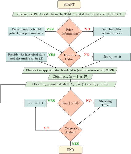To unify notation, we denote by ${\mathit{D}}_n=(\mathit{Y},{\mathit{X}}_n)=(y_1,\dots ,y_{n0},x_1,\dots ,x_n)$ the vector of historical and current data, $\mathit{w}=({\alpha }_0,\dots ,{\alpha }_0,1,\dots ,1)$ the vector of weights corresponding to each element d_j of ${\mathit{D}}_n$ and we call $N_D=n_0+n$ the length of the data vector ${\mathit{D}}_n.$ Technical details regarding the derivation of all these PRC models are available in Appendix A (Supplementary material). Synopsizing the PRC scheme, we provide its flowchart in Figure 1, while in Appendix B (Supplementary material) we present it in an algorithmic form.

Figure 1. PRC flowchart 1. A parallelogram corresponds to an input/output information, a decision is represented by a rhombus and a rectangle denotes an operation after a decision making. In addition, the rounded rectangles indicate the beginning and end of the process.

${}^{★}$For the likelihoods with two unknown parameters and total prior ignorance (i.e. initial reference prior and ${\alpha }_0=0$ in the power prior) we need n = 3 to initiate PRC, while for all other cases, PRC starts right after x₁ becomes available.

3. PRC inference

The control chart associated with PRC has the familiar form of a CUSUM, where the monitoring statistic $S_{n+1}$ (from either (8) or (9)) is plotted versus time with a horizontal decision limit h, that acts as an upper/lower control limit in detecting upward/downward shifts. Issues regarding the design of PRC, like the derivation of h based on false alarm tolerance, along with robustness properties and its illustration in real data applications are covered in Bourazas, Sobas, and Tsiamyrtzis (2023). The area between the horizontal axis and h is considered the IC region, so when $S_{n+1}$ plots beyond the control limit h, then we raise an alarm and our suggestion is to stop the process and examine for an assignable cause, triggering a potential corrective action. From a root cause analysis point of view, a CUSUM alarm will indicate not only that the IC state has been rejected, but it will also offer an estimate of the time where the OOC state was initiated, which is simply the first observation right after the latest time for which we had $S_{n+1}=0.$ Once we correct the problem, then PRC is suggested to be reinitiated, using all past IC recordings as historical data in the power prior.

If we will not react to an alarm, then due to the dynamic update of PRC, OOC data will be involved in the learning process, affecting what is considered IC state. As a result, the monitoring statistic will start moving back to the IC region. This is a well known issue for the self-starting methods, reported in the literature as “window of opportunity” for a control chart to alarm, before the running statistic stops to alarm (in contrast to the fixed parameter CUSUM, where there is no updating and so an alarm will tend to persist). Thus, it is strongly recommended to act upon a PRC alarm.

PRC’s monitoring can be considered a sequential hypothesis testing procedure regarding the unknown parameter. Furthermore, within the Bayesian decision theory framework, one can derive the point/interval estimate of the unknown parameter(s). Precisely, when the process is under the IC state, the posterior distribution of the unknown parameter(s) can be used to derive a Bayes point estimate (like the posterior mean under squared error loss) or the Highest Posterior Density (HPD) credible set. Such inference is also available via the predictive distribution when forecasting might be of interest.

4. Comparative study and sensitivity analysis

PRC is a general self-starting mechanism, aiming to detect small/medium persistent parameter shifts, for any likelihood that is a member of the k-PREF. In this section, we will evaluate its performance and compare it against two of the most prominent competitors: the Cumulative Bayes’ Factors (CBF) of West (1986) and the frequentist alternative, Self-Starting CUSUM (SSC) of Hawkins and Olwell (1998). The comparison will involve data from Normal, Poisson or Binomial, i.e. the most studied distributions in SPC/M. The goal will be to detect as soon as possible, step changes for the mean or inflation for the standard deviation in Normal data (when both parameters are unknown), rate increases in Poisson and increases in the odds of the success probability in Binomial data (all cases refer to typical process deterioration in SPC/M).

All competing methods, are aligned to have identical false alarm rate, while they are designed appropriately to detect the OOC scenario under study. Specifically, we tune the parameter k in PRC, the reference value of SSC, and the discount factor of CBF, to reflect on the size of the shift that we aim to detect. For the SSC with discrete distributions (i.e. Poisson and Binomial) we follow the suggestion (in chapter 7) of Hawkins and Olwell (1998), where the normal scores obtained based on the proposal of Quessenberry (1995a; 1995b) are winsorized by replacing, whenever necessary, the undefined ${\Phi }^{-1}(1)$ by ${\Phi }^{-1}(0.995).$

To derive the decision limit of each method, we simulate 100,000 IC sequences of size N = 50 observations from $N({\theta }_1=0,{\theta }_2^2=1)$ (that will be used for both the mean and the variance charts), $P({\theta }_3=1)$ and $\mathit{Bin}(40,{\theta }_4=0.025).$ In SPC/M we typically use Poisson or Binomial to model count or proportion of defects respectively and so small parameter values are more realistic. Furthermore, the Bayesian PRC and CBF methods require to define a prior distribution and so within this simulation we will take the opportunity to perform a sensitivity analysis, examining the effect of the presence/absence of prior information (reflecting the subjective/non-informative point of view). Therefore, for each scenario, we will compare the SSC against two versions for each of PRC and CBF (with/without prior knowledge). The initial priors ${\pi }_0(·|\mathit{\tau }),$ considered are:

• Normal: reference (non-informative) prior ${\pi }_0({\theta }_1,{\theta }_2^2)\propto 1/{\theta }_2^2\equiv \mathit{NIG}(0,0,-1/2,0)$ or the moderately informative $\mathit{NIG}(0,4,2,1.5).$

• Poisson: reference (non-informative) prior ${\pi }_0({\theta }_3)\propto 1/\sqrt{{\theta }_3}\equiv G(1/2,0)$ or the moderately informative G(4, 4).

• Binomial: reference (non-informative) prior ${\pi }_0({\theta }_4)\propto 1/\sqrt{{\theta }_4(1-{\theta }_4)}\equiv \mathit{Beta}(1/2,1/2)$ or the moderately informative Beta(4, 156).

We should note that in the Normal and Poisson cases, the non-informative priors are improper and for notational convenience are presented as limiting cases of the proper NIG and Gamma distributions respectively.

The OOC scenarios that will evaluate the detection power of the competing methods, come from the 100,000 IC sequences of length N = 50, where small or medium persistent parameter shifts (i.e. step changes) are introduced at one of the locations $\omega =\{11,26\mathrm{ }\text{or}\mathrm{ }41\}.$ In other words, we have three scenarios for the unique change point location ω: either at the start, or in the middle, or near the end of the sample. For each location we will consider two shift sizes, which will be:

• Normal (mean): mean step change of size $\left\{1{\theta }_2\mathrm{ }\text{or}\mathrm{ }1.5{\theta }_2\right\}=\left\{1\mathrm{ }\text{or}\mathrm{ }1.5\right\},$ i.e. after the change point ω, the OOC data come from N(1, 1) or $N(1.5,1).$

• Normal (standard deviation): sd inflation of size $\left\{50\%\mathrm{ }\text{or}\mathrm{ }100\%\right\},$ i.e. after the change point ω, the OOC data come from $N(0,{1.5}^2)$ or $N(0,2^2).$

• Poisson (rate): parameter increase of size $\left\{50\%\mathrm{ }\text{or}\mathrm{ }100\%\right\},$ i.e. after the change point ω, the OOC data come from $P(1.5)$ or P(2).

• Binomial (probability of success): an increase of size $\left\{50\%\mathrm{ }\text{or}\mathrm{ }100\%\right\}$ for the odds of success, i.e. after the change point ω, OOC data come from $\mathit{Bin}(40,0.037)$ or $\mathit{Bin}(40,0.049).$

Next, we provide the performance metrics used to evaluate the competing charts. First, we align all methods to have 5% Family Wise Error Rate (FWER) when we have IC data of length 50, i.e. $\mathit{FWER}(N)=P(T\le N|\omega >N)=0.05,$ where T denotes the stopping time, ω is the time of the step change and N = 50 (length of the data in this study). Regarding OOC detection, the main goal of self-starting methods (especially in short runs), is to be able to ring an alarm before they absorb a change and also minimize the delay in ringing the alarm. The former will be assessed in the same spirit with Frisén (1992) using the Probability of Successful Detection (PSD), where $\mathit{PSD}(\omega )=P(\omega \le T\le N)$ and the bigger $\mathit{PSD}(\omega ),$ the better. For the latter, we estimate the delay of an alarm similar to Kenett and Pollak (2012), using the truncated Conditional Expected Delay, which is $\mathit{tCED}(\omega )=E(T-\omega +1|\omega \le T\le N)$ and it is the average delay of the stopping time, given that this stopping time was after the change point occurrence and before the end of the sample (i.e. point of truncation) and the smaller the delay the better the performance.

The simulation results are summarized graphically in Figure 2 (and analytically in Table S1 of Appendix C, Supplementary material). Overall, the PRC outperforms both competing methods in all scenarios of jump sizes and change point locations, as it has steadily better performance in the detection ability and better or similar performance on the delay in signaling an alarm.

Figure 2. The FWER(k) at each time point $k=2,3,\dots ,50,$ the probability of successful detection, $\mathit{PSD}(\omega )$ and the truncated conditional expected delay, $\mathit{tCED}(\omega )$ for shifts at locations $\omega =\{11,26,41\},$ of SSC, CBF and PRC, under a reference (CBF_r, PRC_r) or a moderately informative (CBF_mi, PRC_mi) prior. The results refer to Normal data with step changes for the mean of size $\{1{\theta }_2,1.5{\theta }_2\},$ Normal data with inflated standard deviation of size $\{50\%,100\%\},$ Poisson data with rate increase of size $\{50\%,100\%\}$ and Binomial data with increase for the odds of size $\{50\%,100\%\}.$

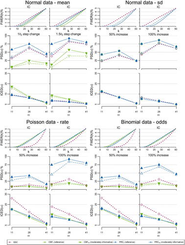
Initially, for the detection performance within each method, we observe (as it was expected) that the bigger the size of the shift, the higher the detection power. Regarding the effect of the location ω, we observe that in all cases the best performance appears when the change point is at the middle of the sequence (ω = 26). The lower performance in the start (ω = 11), is related to the fact that the learning process is not as mature as in the middle of the sequence. For the change near the end (ω = 41) despite the fact that the learning has been significantly improved the performance decreases as there is not sufficiently long time to build up the evidence and ring an alarm (there exist only $50-\omega +1=10$ observations until we reach the end of the data sequence).

Comparing across methods via $\mathit{PSD}(\omega ),$ we observe that the PRC achieves higher detection percentage than SSC for all distributions, shifts and locations. The PRC’s outperformance against SSC is valid irrespectively of whether we have an informative or not prior distribution and their difference is greater at ω = 11 (the earlier the shift the bigger the difference). The SSC’s significantly lower performance versus PRC (even when a reference prior is in use) in the discrete distributions can be attributed to the fact that SSC is using an approximation to normality algorithm that in discrete data can be poor. The CBF, with one exception, is having the lowest performance of all competing methods. This is the price that CBF pays for aiming to be general and not specifying a target OOC distribution (it simply diffuses the predictive distribution keeping the same location). The exception is when we study shifts in the standard deviation of the normal data, where the CBF becomes informative, since the alternative (OOC) scenario involves the same location and inflated variance. Thus, for this specific scenario, CBF coincides with PRC providing identical performance and in a way indicating that CBF is a method focusing in scale shifts.

Regarding $\mathit{tCED}(\omega ),$ we observe that PRC is indifferent from SSC in Normal data (and better from CBF in normal mean PRC), while for the discrete distributions we have PRC to have comparable performance with CBF and a lot better (i.e. smaller delay) when compared to the SSC.

Finally, the prior sensitivity indicates that even moderately informative prior information enhances the performance of PRC (and CBF). This is more intense at the early stages of the process (ω = 11), when the volume of the data is very low.

5. Conclusions

In this work a Bayesian change point model, PRC, is suggested for scenarios where we aim to detect in an online fashion, persistent parameter shifts of small/medium size in short production runs. The methodological framework is given in a general form providing a platform able to accommodate any univariate data generating distribution that belongs to the regular exponential family. Furthermore, the use of power priors allows to incorporate possibly available historical data along with subjective initial prior information (or a non-informative initial prior when we lack prior knowledge), boosting the performance at the early stages.

PRC is an enhanced Bayesian version of the frequentist SSC. In addition, PRC utilizes the fact that the alternative (competing) models (OOC in the SPC/M framework) are known, providing a method that improves significantly the CBF approach, whose modeling structure works only in scale parameter shifts. A detailed simulation, evaluating the detection (both in power and alarm delay) of persistent shifts, shows that PRC outperforms SSC even when a non-informative prior is used and it is also more powerful from CBF, except the special case where we look for shifts in the variance of a location scale family distribution, where CBF coincides with PRC.

The PRC methodology was developed as a self starting quality monitoring scheme, within the SPC/M area and as such it can be used in a variety of disciplines, industrial or not (like medical laboratories, economic, geological etc.). Overall, it is a tool focusing in online detection of persistent parameter shifts, especially when only low volume of data is available (short runs or online phase I data analysis). Apart from the change point detection aspect of PRC (i.e. alarm a shift and provide an estimate of when this shift was originated), thanks to the Bayesian framework, at each time we can have a point/interval estimate of the unknown parameter, which will be sequentially updated. Finally, the detailed description of the methodology in closed form allows its straightforward implementation in either short or long sequences of data.

Acknowledgments

We are grateful to the Editor and all reviewers for their excellent work. Their constructive criticism and suggestions, improved significantly the quality of this manuscript. This research was partially funded by the international company Instrumentation Laboratory (IL), Bedford, Massachusetts, USA and the Research Center of the Athens University of Economics and Business (AUEB).

Additional information

Funding

This work was supported by Research Center of the Athens University of Economics and Business (RC/AUEB) and Instrumentation Laboratory (IL), Bedford, Massachusetts, USA.

Notes on contributors

Konstantinos Bourazas

Dr. Konstantinos Bourazas received his Ph.D. from the Department of Statistics, at the Athens University of Economics and Business, Greece. He is currently a postdoctoral researcher at the Department of Mathematics & Statistics at the University of Cyprus, as well as participating in an interdepartmental research project at the University of Ioannina, Greece. His research interests are in the areas of Statistical Process Control and Monitoring, Bayesian Statistics, Change Point Models, Replication Studies and Applied Statistics.

Frederic Sobas

Dr. Frederic Sobas is specialized in hemostasis. He is a clinical chemist graduated from Claude Bernard University Lyon I, France. He is a Quality Manager focusing in medical laboratories accreditation issues with respect to ISO 15189 norm.

Panagiotis Tsiamyrtzis

Panagiotis Tsiamyrtzis is an Associate Professor at the Department of Mechanical Engineering, Politecnico di Milano and his email is [email protected].

References

- Ali, S. 2020. A predictive Bayesian approach to EWMA and CUSUM charts for time-between-events monitoring. Journal of Statistical Computation and Simulation 90 (16):3025–50. doi: 10.1080/00949655.2020.1793987.
- Berger, J. O., J. M. Bernardo, and D. Sun. 2009. The formal definition of reference priors. Annals of Statistics 37:905–38.
- Bernardo, J. M. 1979. Reference posterior distributions for Bayesian inference. Journal of the Royal Statistical Society Series B (Methodological 41 (2):113–28. doi: 10.1111/j.2517-6161.1979.tb01066.x.
- Bernardo, J. M., and A. F. M. Smith. 2000. Bayesian Theory. 1st ed. New York: Wiley.
- Bourazas, K., D. Kiagias, and P. Tsiamyrtzis. 2022. Predictive Control Charts (PCC): A Bayesian approach in online monitoring of short runs. Journal of Quality Technology 54 (4):367–391. doi:10.1080/00224065.2021.1916413.
- Bourazas, K., F. Sobas, and P. Tsiamyrtzis. 2023. Design and properties of the Predictive Ratio Cusum (PRC) control charts. Journal of Quality Technology, online advance. doi: 10.1080/00224065.2022.2161435
- Capizzi, G., and G. Masarotto. 2013. Phase I distribution-free analysis of univariate data. Journal of Quality Technology 45 (3):273–84. doi: 10.1080/00224065.2013.11917938.
- Deming, W. E. 1986. Out of crisis. Massachusetts: The MIT Press.
- Frisén, M. 1992. Evaluations of methods for statistical surveillance. Statistics in Medicine 11 (11):1489–502. doi: 10.1002/sim.4780111107.
- Gelman, A. (2006). Prior distributions for variance parameters in hierarchical models (comment on article by Browne and Draper). Bayesian analysis 1 (3):515–534.
- Hawkins, D. M., and D. H. Olwell. 1998. Cumulative sum charts and charting for quality improvement. New York: Springer-Verlag.
- Ibrahim, J., and M. Chen. 2000. Power prior distributions for regression models. Statistical Science 15:46–60.
- Jones-Farmer, L. A., W. H. Woodall, S. H. Steiner, and C. W. Champ. 2014. An overview of phase I analysis for process improvement and monitoring. Journal of Quality Technology 46 (3):265–80. doi: 10.1080/00224065.2014.11917969.
- Kass, R. E., and A. E. Raftery. 1995. Bayes factors. Journal of the American Statistical Association 90 (430):773–95. doi: 10.1080/01621459.1995.10476572.
- Kenett, R. S., and M. Pollak. 2012. On assessing the performance of sequential procedures for detecting a change. Quality and Reliability Engineering International 28 (5):500–7. doi: 10.1002/qre.1436.
- Page, E. S. 1954. Continuous inspection schemes. Biometrika 41 (1-2):100–15. doi: 10.1093/biomet/41.1-2.100.
- Qiu, P. 2014. Introduction to statistical process control. Boca Raton, FL: CRC Press, Chapman & Hall.
- Quesenberry, C. P. (1995a). On properties of binomial Q charts for attributes. Journal of Quality Technology 27 (3):204–213.
- Quesenberry, C. P. (1995b). On properties of Poisson Q charts for attributes. Journal of Quality Technology 27 (4): 293–303.
- Roberts, S. W. 1959. Control chart tests based on geometric moving averages. Technometrics 1 (3):239–50. doi: 10.1080/00401706.1959.10489860.
- Roberts, S. W. 1966. A comparison of some control chart procedures. Technometrics 8 (3):411–30. doi: 10.1080/00401706.1966.10490374.
- Shewhart, W. H. 1926. Quality control charts. Bell System Technical Journal 5 (4):593–603. doi: 10.1002/j.1538-7305.1926.tb00125.x.
- Shiryaev, A. 1963. On optimum methods in quickest detection problems. Theory of Probability & Its Applications 8 (1):22–46. doi: 10.1137/1108002.
- Tsiamyrtzis, P., and D. M. Hawkins. 2005. A Bayesian scheme to detect changes in the mean of a short run process. Technometrics 47 (4):446–56. doi: 10.1198/004017005000000346.
- Tsiamyrtzis, P., and D. M. Hawkins. 2010. Bayesian start up phase mean monitoring of an autocorrelated process that is subject to random sized jumps. Technometrics 52 (4):438–52. doi: 10.1198/TECH.2010.08053.
- Tsiamyrtzis, P., and D. M. Hawkins. 2019. Statistical process control for Phase I count type data. Applied Stochastic Models in Business and Industry 35 (3):766–87. doi: 10.1002/asmb.2398.
- West, M. 1986. Bayesian model monitoring. Journal of the Royal Statistical Society: Series B (Methodological) 48 (1):70–8.
- West, M., and P. J. Harrison. 1986. Monitoring and adaptation in Bayesian forecasting models. Journal of the American Statistical Association 81 (395):741–50. doi: 10.1080/01621459.1986.10478331.
- Woodward, P. W., and J. C. Naylor. 1993. An application of Bayesian methods in SPC. The Statistician 42 (4):461–9. doi: 10.2307/2348478.