A review and comparison of control charts for ordinal samples

Abstract

Qualitative, more specifically, ordinal data generating processes are common in real-world process control implementations. In this study, a survey of control charts for the sample-based monitoring of independent and identically distributed ordinal data is provided together with critical comparisons of the control statistics, for memory-less Shewhart-type and for memory-utilizing exponentially weighted moving average (EWMA) and cumulative-sum types of control charts. New results and proposals are also provided for process monitoring. Using some real-world quality scenarios from the literature, a simulation study for performance comparisons is conducted, covering sixteen different types of control chart. It is shown that demerit-type charts used in combination with EWMA smoothing generally perform better than the other charts, which may rely on quite sophisticated derivations. A real-world data example for monitoring flashes in electric toothbrush manufacturing is discussed to illustrate the application and interpretation of the control charts in the study.

Keywords:

• attributes control charts
• average run length
• ordinal data
• statistical process control

1. Introduction

Control charts are an important tool of statistical process control (SPC), which are used for monitoring quality-related processes. Most of the SPC literature focuses on the case where the relevant quality characteristics are measured on a quantitative scale, such as real-valued measurements or integer-valued counts (Montgomery 2009). Recently, there has been increasing interest in monitoring qualitative data (Weiß 2021a). In particular, ordinal data can be found in many SPC applications, i.e., data generated by some random variable X, the range of which consists of finitely many categories exhibiting a natural order¹. We denote the range of X as $\mathcal{S}=\{s_0,s_1,\dots ,s_d\}$ with some $d\in \mathbb{N}=\{1,2,\dots \},$ where $s_0<s_1<\dots <s_d.$ The monitoring of ordinal data is not only relevant in manufacturing (e.g., severity of a defect) and the service industry (e.g., perceived quality of service), but also in non-industrial areas such as health surveillance (e.g., surgical performance) as well as climatological (e.g., wind force) and environmental applications (e.g., air quality). In the following, we focus on control charts applied to independent and identically distributed (i.i.d.) samples of univariate ordinal data. Note that there are also a few contributions concerning multivariate ordinal data, ordinal time series, or continuous monitoring of individual ordinal observations (see Weiß (2021a) for references). However, as the majority of publications consider sample-based monitoring of i.i.d. ordinal data and to keep the scope of the present study manageable, we concentrate on univariate ordinal samples, while recommending more studies on the aforementioned topics for future research in Section 6.

In Section 2, we introduce the required concepts and notations for this research. In Section 3, we survey (and complement by some new proposals) important types of control charts for i.i.d. ordinal samples, which are classified in the following groups: Section 3.1 presents control charts, where the monitored statistic is a quadratic form in the sample frequencies, with weights being derived from ordinal principles. In Section 3.2, the monitored statistic is a weighted class count, where the weights are either determined based on a demerit scheme, or they follow from some probabilistic reasoning. In Section 3.3, statistics from ordinal data analysis are monitored, such as ordinal dispersion, and Section 3.4 concludes the survey with some references on further approaches that have been proposed in the literature so far. Section 4 provides an extensive performance analysis, where the main charts from Section 3 are compared to each other regarding their average run length (ARL) properties. There, we consider both medium- and high-quality scenarios, where the considered in-control models are inspired by real applications that have previously been reported in the literature. The application and interpretation of the control charts in practice are illustrated by a real-world data example in Section 5, where a manufacturing process of electric toothbrushes is monitored. Finally, Section 6 concludes the article and outlines directions for future research.

2. Basic concepts and notations

In this research, we assume the tth sample of size n > 1 (one may also consider time-varying sample sizes n_t) to consist of the i.i.d. ordinal random variables $X_{t,1},\dots ,X_{t,n}$ with range $\mathcal{S},$ and the different samples are assumed to be mutually independent as well. The stochastic properties of $X_{t,i}$ are fully specified by its probability mass function (PMF), $\mathit{p}=(p_0,\dots ,p_d)\in {[0;1]}^{d+1}$ with $p_i=P(X=s_i).$ In order to account for the natural order among the categories, it is actually more common to consider the cumulative distribution function (CDF) instead (Agresti 2010), given by $\mathit{f}=(f_0,\dots ,f_{d-1})\in {[0;1]}^d$ with $f_i=P(X\le s_i).$ Note that f_d is omitted in f as f_d = 1 always holds.

2.1. Basics of process monitoring

We declare the monitored process to be in control as long as it follows the specified in-control distribution, given by ${\mathit{p}}_0$ and ${\mathit{f}}_0,$ respectively. If the sample at time $t=\tau$ is the first one with distribution being different to ${\mathit{p}}_0,{\mathit{f}}_0,$ then τ is said to be a change point, and the process is called out of control for $t\ge \tau .$ In SPC, a control chart is applied to the samples $\left\{X_{t,i}\right\}$ by sequentially computing a certain statistic for each sampling time $t=1,2,\dots ,$ and these statistics are used to decide about the state of the process: if a statistic exceeds the given control limits (CLs), an alarm is triggered and entails an inspection of the process for a possible out-of-control situation. Obviously, we do not wish to intervene in the process if this is in control (false alarm, i.e., if $t<\tau$), while a true change ($t\ge \tau$) should be detected as soon as possible. A common way of evaluating a control chart’s performance with respect to these two opposing poles is to compute its ARL for a given scenario, i.e., the mean time until the first alarm is triggered. The ARL should be large if the process is in control, whereas it should be small if the process is out of control. For these and further basics on SPC and control charts, see the textbook by Montgomery (2009).

The fundamental idea behind an ordinal control chart is to compare (sequentially) the information provided by the tth sample $\left\{X_{t,i}\right\}$ to the in-control model as given by ${\mathit{p}}_0,{\mathit{f}}_0.$ The full information on the sample $\left\{X_{t,i}\right\},$ in turn, is comprised by the corresponding vectors of frequencies and cumulative frequencies, ${\mathit{N}}_t=(N_{t,0},\dots ,N_{t,d})$ and ${\mathit{C}}_t=(C_{t,0},\dots ,C_{t,d-1}),$ respectively, where $N_{t,j}$ expresses the number of $X_{t,i}=s_j$ in the sample, and $C_{t,j}$ the number of $X_{t,i}\le s_j.$ If the distribution of $\left\{X_{t,i}\right\}$ is given by $\mathit{p},\mathit{f},$ we have $E[{\mathit{N}}_t]=n·\mathit{p}$ and $E[{\mathit{C}}_t]=n·\mathit{f}.$ Thus, the corresponding vectors of relative (cumulative) frequencies, ${\widehat{\mathit{p}}}_t=\frac{1}{n} {\mathit{N}}_t$ and ${\widehat{\mathit{f}}}_t=\frac{1}{n} {\mathit{C}}_t,$ are unbiased estimators of p and f, respectively. For the control charts considered in this article, the tth statistic is either a function of solely ${\mathit{N}}_t,$ say $g({\mathit{N}}_t),$ then it constitutes a (memory-less) Shewhart chart, or it is a function of the ${\mathit{N}}_1,\dots ,{\mathit{N}}_t$ being available up to time t, say $h({\mathit{N}}_1,\dots ,{\mathit{N}}_t),$ then we are concerned with a control chart having an inherent memory. Note that by appropriately modifying g, h, we could equivalently use ${\mathit{C}}_t,{\widehat{\mathit{p}}}_t,$ or ${\widehat{\mathit{f}}}_t$ instead of ${\mathit{N}}_t$ to express these statistics. Popular examples for constructing memory-type control charts are the cumulative sum (CUSUM) concept dating back to Page (1954), and the exponentially weighted moving-average (EWMA) concept dating back to Roberts (1959). In the ordinal case, a widely-used approach for generating a memory-type chart is to apply EWMA smoothing to the process of frequency vectors, e.g., to ${({\mathit{N}}_t)}_{t\in \mathbb{N}}:$ for given smoothing parameter $\lambda \in (0;1),$ one computes [2.1] $${\mathit{N}}_t^{(\lambda )}=\lambda {\mathit{N}}_t+(1-\lambda ) {\mathit{N}}_{t-1}^{(\lambda )}\hspace{1em}\text{for}\mathrm{ }t=1,2,\dots ,\mathrm{\hspace{1em}}\mathrm{\hspace{1em}}{\mathit{N}}_0^{(\lambda )}=n {\mathit{p}}_0.$$[2.1]

Then, the monitored statistic is computed as $g({\mathit{N}}_t{}^{(\lambda )})$ for $t=1,2,\dots ,$ whereas the corresponding Shewhart version monitors $g({\mathit{N}}_t)$ instead, see Li, Tsung, and Zou (2014); Wang, Su, and Xie (2018); Bai and Li (2021) for such examples. Possible adoptions of the CUSUM approach to the case of ordinal data are described later in Section 3.2.

Remark 2.1.1.

The term “ARL” is not uniquely defined in the literature, but there are competing approaches, see Knoth (2006). The default concept is the zero-state ARL, where it is assumed that the possible process change happens with the start of process monitoring, i.e., τ = 1. Other concepts such as the steady-state ARL assume a delayed change point. In this research, we are concerned with independent samples ${\mathit{N}}_1,{\mathit{N}}_2,\dots$ Consequently, if applying a Shewhart-type chart to ${\mathit{N}}_1,{\mathit{N}}_2,\dots ,$ then all these ARL concepts coincide. For memory-type control charts, the obtained ARL values usually differ. But, it is widely known that the well-established CUSUM and EWMA charts lead to only modest differences with no practical implications in the independence scenario considered here. Therefore, in what follows, we focus on zero-state ARLs and omit a discussion of further ARL concepts.

2.2. Parametric models for ordinal data

For performance analyses of control charts, it is useful to have parametric models for an ordinal random variable X, which allows for modifications of the relevant distributional properties, such as the location or dispersion of X. There are only few “direct” proposals on parametric distributions for the ordinal X; instead, it is more common to derive an ordinal distribution from either an underlying discrete count distribution, or from a continuous real-valued distribution. A tailor-made proposal for the ordinal X is the “λ-μ-distribution” of (Kvålseth 2011a, Section 5), which is defined as [2.2] $$\mathit{p}=((1-\frac{1}{2} \mu ) (1-\lambda )+\frac{1}{d+1} \lambda ,\frac{1}{d+1} \lambda ,\dots ,\frac{1}{d+1} \lambda ,\frac{1}{2} \mu (1-\lambda )+\frac{1}{d+1} \lambda )$$[2.2] for $\lambda ,\mu \in [0;1].$ It comprises the most relevant extreme scenarios for qualitative random variables:

• $\mu =\lambda =0:$ the one-point distribution $\mathit{p}=(1,0,\dots ,0)$ or $\mathit{f}=(1,\dots ,1),$ respectively, i.e., the case of minimal qualitative dispersion (maximal consensus);

• λ = 1: the uniform distribution $\mathit{p}=(\frac{1}{d+1},\dots ,\frac{1}{d+1})$ or $\mathit{f}=(\frac{1}{d+1},\dots ,\frac{d}{d+1}),$ respectively, i.e., the case of maximal nominal dispersion (maximal uncertainty);

• μ = 1 and λ = 0: the extreme two-point distribution (polarized distribution) $\mathit{p}=(\frac{1}{2},0,\dots ,0,\frac{1}{2})$ or $\mathit{f}=(\frac{1}{2},\dots ,\frac{1}{2}),$ respectively, i.e., the case of maximal ordinal dispersion (maximal dissent).

Also, the “Lehmann approach” (Lehmann 1953; Klein and Doll 2021) should be mentioned as a possibility for achieving parametric ordinal models: starting from some baseline CDF f, one considers the CDF ${\mathit{f}}^{\alpha }$ with component-wise exponent $\alpha >0.$ But as mentioned before, it is more common to derive a parametric model for the ordinal X from some underlying quantitative model. One such approach was referred to as rank counts by Weiß (2020), where the probabilities in p are assumed to be equal to those of a chosen parametric distribution for bounded counts with range $\{0,\dots ,d\},$ such as a binomial (Bin), beta-binomial (BB), or k-inflated binomial (k-IB) distribution with upper bound d. Thus, the shape of p is controlled by one or two parameters. This can be formalized by writing X = s_I, where the random rank count I follows a discrete bounded-counts distribution. For example, if $I\sim k-\text{IB}(d,\pi ,\omega )$ with $\pi ,\omega \in [0;1]$ and $k\in \{0,\dots ,d\},$ then this implies that [2.3] $$P(X=s_j)=\omega ·1(j=k)+(1-\omega )·\left(\begin{array}{c}d\\ j\end{array}\right) {\pi }^j {(1-\pi )}^{d-j},$$[2.3] where $1(A)$ denotes the indicator function, which equals 1 (0) if A is true (false). Note that (2.3) reduces to the PMF of $\text{Bin}(d,\pi )$ if ω = 0. As an example, if k = 0 (zero inflation), then we get the one-point distribution $\mathit{p}=(1,0,\dots ,0)$ for ω = 1, while $\omega =\frac{1}{2}$ and π = 1 leads to the extreme two-point distribution.

Another approach to derive a parametric model for the ordinal X is the assumption of a real-valued latent variable Q (Agresti 2010, p. 11), which follows a specified continuous distribution; let $F_Q(x)$ denote the corresponding CDF. Then, threshold parameters $-\infty ={\eta }_{-1}<{\eta }_0<\dots <{\eta }_{d-1}<{\eta }_d=+\infty$ have to be specified, and one defines [2.4] $$P(X=s_j)=F_Q({\eta }_j)-F_Q({\eta }_{j-1})\mathrm{\hspace{1em}}\mathrm{\hspace{1em}}\text{for}\mathrm{ }j=0,\dots ,d.$$[2.4]

Popular choices for F_Q are the (standard) logistic (Log) or normal (N) distribution, leading to the ordered logit or probit model, respectively. While Q is typically assumed to exist only virtually (thus “latent”), there are some applications where Q also has a physical meaning, e.g., if grouped data resulting from gauging are used instead of exact measurements, see Steiner, Geyer, and Wesolowsky (1994, 1996a,1996b).

3. Control charts for ordinal samples

This section provides a broad survey of existing control charts for i.i.d. ordinal samples, supplemented by a few new results and proposals. Doing this, we identified groups of more general monitoring concepts and classified the control charts into these groups. As the groups are not perfectly disjoint, we shall point out if a control chart could be assigned to another group as well.

3.1. Ordinal quadratic-form statistics

One of the earliest proposals for the monitoring of i.i.d. qualitative samples $\left\{X_{t,i}\right\}$ is a Shewhart-type control chart relying on Pearson’s goodness-of-fit (GoF) statistic [3.1] $${\mathrm{X}}_t^2=\sum _{j=0}^d\frac{{(N_{t,j}-n p_{0,j})}^2}{n p_{0,j}}=n^{-1} {({\mathit{N}}_t-n {\mathit{p}}_0)}^{\top } \mathrm{ }\text{diag}{({\mathit{p}}_0)}^{-1} ({\mathit{N}}_t-n {\mathit{p}}_0).$$[3.1]

The second representation shows that ${\mathrm{X}}_t^2$ constitutes a particular type of quadratic form in ${\mathit{N}}_t$ or ${\widehat{\mathit{p}}}_t,$ respectively. The idea of monitoring $({\mathrm{X}}_t^2)$ can be traced back to (Shewhart 1931, p. 329), while the first comprehensive discussion appears to be in Duncan (1950). Ordinal applications of [3.1[3.1] $${\mathrm{X}}_t^2=\sum _{j=0}^d\frac{{(N_{t,j}-n p_{0,j})}^2}{n p_{0,j}}=n^{-1} {({\mathit{N}}_t-n {\mathit{p}}_0)}^{\top } \mathrm{ }\text{diag}{({\mathit{p}}_0)}^{-1} ({\mathit{N}}_t-n {\mathit{p}}_0).$$[3.1] ] are presented by Marcucci (1985); Wardell and Candia (1996); Edwards, Govindaraju, and Lai (2007); Samimi, Aghaie, and Tarokh (2010). Obviously, [3.1[3.1] $${\mathrm{X}}_t^2=\sum _{j=0}^d\frac{{(N_{t,j}-n p_{0,j})}^2}{n p_{0,j}}=n^{-1} {({\mathit{N}}_t-n {\mathit{p}}_0)}^{\top } \mathrm{ }\text{diag}{({\mathit{p}}_0)}^{-1} ({\mathit{N}}_t-n {\mathit{p}}_0).$$[3.1] ] is not limited to ordinal data, but can be used for qualitative data in general. However, its application to specifically ordinal data can be justified as detailed in Appendix B. There, it is shown that ${\mathrm{X}}_t^2$ can be equivalently expressed as a quadratic form in the CDF ${\widehat{\mathit{f}}}_t,$ see (B.1), which, as explained in Section 2, accounts for the natural order among the categories through the accumulation. In other words: even if one defines the quadratic-form statistic (B.1) in an explicitly ordinal manner, we end up with the traditional Pearson statistic [3.1[3.1] $${\mathrm{X}}_t^2=\sum _{j=0}^d\frac{{(N_{t,j}-n p_{0,j})}^2}{n p_{0,j}}=n^{-1} {({\mathit{N}}_t-n {\mathit{p}}_0)}^{\top } \mathrm{ }\text{diag}{({\mathit{p}}_0)}^{-1} ({\mathit{N}}_t-n {\mathit{p}}_0).$$[3.1] ] anyway.

To establish a closer connection to ordinal data, the Pearson statistic [3.1[3.1] $${\mathrm{X}}_t^2=\sum _{j=0}^d\frac{{(N_{t,j}-n p_{0,j})}^2}{n p_{0,j}}=n^{-1} {({\mathit{N}}_t-n {\mathit{p}}_0)}^{\top } \mathrm{ }\text{diag}{({\mathit{p}}_0)}^{-1} ({\mathit{N}}_t-n {\mathit{p}}_0).$$[3.1] ] can be extended to a weighted quadratic-form statistic, where the weights account for the ordering among the categories. This was proposed by Wang, Su, and Xie (2018), whose average cumulative data (ACD) chart relies on [3.2] $${\text{ACD}}_t=n^{-1} ({\mathit{N}}_t-n {\mathit{p}}_0){\mathrm{}}^{\top } \mathbf{V} ({\mathit{N}}_t-n {\mathit{p}}_0),$$[3.2] where V denotes a given weight matrix. Obviously, the Pearson statistic [3.1[3.1] $${\mathrm{X}}_t^2=\sum _{j=0}^d\frac{{(N_{t,j}-n p_{0,j})}^2}{n p_{0,j}}=n^{-1} {({\mathit{N}}_t-n {\mathit{p}}_0)}^{\top } \mathrm{ }\text{diag}{({\mathit{p}}_0)}^{-1} ({\mathit{N}}_t-n {\mathit{p}}_0).$$[3.1] ] follows if choosing $\mathbf{V}=\text{diag}{({\mathit{p}}_0)}^{-1}.$ Wang, Su, and Xie (2018) suggest to use $\mathbf{V}={\mathbf{L}}^{\top } \text{diag}(\mathit{w}) \mathbf{L}$ with weight vector w, where L has a triangular structure: the lower (upper) triangle is filled with 2 (0), and the main diagonal with 1. In this case, setting $C_{t,-1}=f_{0,-1}=0,$ ${\text{ACD}}_t$ calculates as [3.3] $${\text{ACD}}_t=n^{-1} \sum _{j=0}^d{w}_j {(C_{t,j-1}+C_{t,j}-n (f_{0,j-1}+f_{0,j}))}^2,$$[3.3] i.e., it is a quadratic form in the average cumulative proportions $\frac{1}{2} (f_{0,j-1}+f_{0,j}),$ the so-called “ridits” (Agresti 2010, p. 10). This artificial word was created by Bross (1958) in analogy to “logit” and “probit” (recall Section 2.2), where “rid” expresses “relative to an identified distribution”. The weight vector w might simply be chosen as $\mathit{w}=\mathbf{1}={(1,\dots ,1)}^{\top }$ (Wang, Su, and Xie 2018, p. 119) if there is no reason for a more sophisticated weighting scheme.

Another weighted quadratic-form scheme is the univariate location-scale ordinal (ULSO) control chart recently proposed by Bai and Li (2021), where the weights are derived from the latent-variable approach [2.4[2.4] $$P(X=s_j)=F_Q({\eta }_j)-F_Q({\eta }_{j-1})\mathrm{\hspace{1em}}\mathrm{\hspace{1em}}\text{for}\mathrm{ }j=0,\dots ,d.$$[2.4] ]. It can be expressed as that ACD chart [3.2[3.2] $${\text{ACD}}_t=n^{-1} ({\mathit{N}}_t-n {\mathit{p}}_0){\mathrm{}}^{\top } \mathbf{V} ({\mathit{N}}_t-n {\mathit{p}}_0),$$[3.2] ], where [3.4] $$\mathbf{V}={\mathbf{Q}}^{\top } {(\mathbf{Q} (\text{diag}({\mathit{p}}_0)-{\mathit{p}}_0 {\mathit{p}}_0^{\top }) {\mathbf{Q}}^{\top })}^{-1} \mathbf{Q}.$$[3.4]

If using the cumulative logit approach as recommended by (Bai and Li 2021, p. 941), the $2\times (d+1)$-matrix $\mathbf{Q}=(q_{kl})$ has the entries $$q_{1j}=f_{0,j-1}+f_{0,j}-1,\hspace{1em}{q}_{2j}=p_{0,j}^{-1} (\eta (f_{0,j})-\eta (f_{0,j-1}))\hspace{1em}\text{for}\mathrm{ }j=0,\dots ,d,$$ where $\eta (z)=z(1-z) \hspace{0.17em}\ln \hspace{0.17em}((1-z)/z)$ with $\eta (0)=\eta (1)=0.$ Thus, the “location scores” $q_{1j}$ again rely on ridits, whereas the structure of the “scale scores” $q_{2j}$ is a consequence of the cumulative logit approach (remind Section 2.2). Note that [3.4[3.4] $$\mathbf{V}={\mathbf{Q}}^{\top } {(\mathbf{Q} (\text{diag}({\mathit{p}}_0)-{\mathit{p}}_0 {\mathit{p}}_0^{\top }) {\mathbf{Q}}^{\top })}^{-1} \mathbf{Q}.$$[3.4] ] is well defined only if $d\ge 2,$ and that the ULSO statistic reduces to the ordinary Pearson statistic [3.1[3.1] $${\mathrm{X}}_t^2=\sum _{j=0}^d\frac{{(N_{t,j}-n p_{0,j})}^2}{n p_{0,j}}=n^{-1} {({\mathit{N}}_t-n {\mathit{p}}_0)}^{\top } \mathrm{ }\text{diag}{({\mathit{p}}_0)}^{-1} ({\mathit{N}}_t-n {\mathit{p}}_0).$$[3.1] ] if d = 2; see Appendix C for details. Thus, non-trivial ULSO charts are only available if $d\ge 3$ (i.e., if the range of X consists of at least four categories).

Finally, let us recall that the Shewhart versions of the quadratic-form control charts [3.1[3.1] $${\mathrm{X}}_t^2=\sum _{j=0}^d\frac{{(N_{t,j}-n p_{0,j})}^2}{n p_{0,j}}=n^{-1} {({\mathit{N}}_t-n {\mathit{p}}_0)}^{\top } \mathrm{ }\text{diag}{({\mathit{p}}_0)}^{-1} ({\mathit{N}}_t-n {\mathit{p}}_0).$$[3.1] ] to [3.4[3.4] $$\mathbf{V}={\mathbf{Q}}^{\top } {(\mathbf{Q} (\text{diag}({\mathit{p}}_0)-{\mathit{p}}_0 {\mathit{p}}_0^{\top }) {\mathbf{Q}}^{\top })}^{-1} \mathbf{Q}.$$[3.4] ] are easily equipped with an inherent memory by substituting the raw frequencies ${\mathit{N}}_t$ by the smoothed frequencies ${\mathit{N}}_t{}^{(\lambda )}$ according to [2.1[2.1] $${\mathit{N}}_t^{(\lambda )}=\lambda {\mathit{N}}_t+(1-\lambda ) {\mathit{N}}_{t-1}^{(\lambda )}\hspace{1em}\text{for}\mathrm{ }t=1,2,\dots ,\mathrm{\hspace{1em}}\mathrm{\hspace{1em}}{\mathit{N}}_0^{(\lambda )}=n {\mathit{p}}_0.$$[2.1] ]. This was suggested by Wang, Su, and Xie (2018); Bai and Li (2021) for their ACD and ULSO charts, respectively, but it can also be applied to the Pearson statistic [3.1[3.1] $${\mathrm{X}}_t^2=\sum _{j=0}^d\frac{{(N_{t,j}-n p_{0,j})}^2}{n p_{0,j}}=n^{-1} {({\mathit{N}}_t-n {\mathit{p}}_0)}^{\top } \mathrm{ }\text{diag}{({\mathit{p}}_0)}^{-1} ({\mathit{N}}_t-n {\mathit{p}}_0).$$[3.1] ] as well as to the Shewhart-type charts being discussed in later sections.

3.2. Statistics based on weighted class counts

Several control charts rely on a type of weighted class count, i.e., a statistic of the form [3.5] $$D_t=v_0 N_{t,0} +\cdots + v_d N_{t,d},$$[3.5] which is plotted against a lower and upper CL (LCL and UCL, respectively). Statistic [3.5[3.5] $$D_t=v_0 N_{t,0} +\cdots + v_d N_{t,d},$$[3.5] ] corresponds to taking the sample sum after having transformed the original ordinal range $\mathcal{S}$ into a range of numerical scores, $\mathcal{V}=\{v_0,\dots ,v_d\}.$ There are two common ways of choosing the scores in practice: one may define the scores based on probabilistic arguments, as detailed below, or one chooses the scores based on “external reasoning”, which is first discussed in the present section. In a quality context, such scores are typically chosen to express the severity of defects, leading to a demerit control chart. Such demerit charts date back to Dodge (1928); Dodge and Torrey (1956) and have been further investigated by, among others, Jones, Woodall, and Conerly (1999) and (Montgomery 2009, Section 7.3.3). In the latter two references, the default example refers to $d+1=4$ levels of defect, ranging from class D (“not serious”) to A (“very serious”) with corresponding demerit values $1,10,50,100.$ Another example is reported by Nembhard and Nembhard (2000), where $d+1=3$ classes of nonconformity (minor, major, critical) are assigned the scores 1, 3, 10. Finally, in Wardell and Candia (1996), the scores regarding customer satisfaction are simply chosen as the integers $1,\dots ,d+1$ (Likert scale) — this particular choice shall be discussed again in Section 3.3.

Although common in practice, the approach of choosing numerical scores for ordinal data (and thus implicitly using a metric scale) is criticized by (Agresti 2010, p. 10), because “often, an appropriate choice of scores is unclear” and the obtained outcome might be sensitive to the actual choice of the scores. Applied to the context of SPC, the question arises if there is a notable effect of this choice on the ARL performance of the demerit chart [3.5[3.5] $$D_t=v_0 N_{t,0} +\cdots + v_d N_{t,d},$$[3.5] ].

Therefore, an alternative approach is to derive the weights $v_0,\dots ,v_d$ in [3.5[3.5] $$D_t=v_0 N_{t,0} +\cdots + v_d N_{t,d},$$[3.5] ] from probabilistic principles. There are several suggestions in the literature on how to choose these scores in this way. The so-called simple ordinal categorical (SOC) chart of Li, Tsung, and Zou (2014) plots the absolute values of [3.5[3.5] $$D_t=v_0 N_{t,0} +\cdots + v_d N_{t,d},$$[3.5] ], where the weights v_j are related to the ridits of the in-control distribution: [3.6] $${\text{SOC}}_t=|\sum _{j=0}^d(f_{0,j-1}+f_{0,j}-1) N_{t,j}|\hspace{1em}\text{with}\mathrm{ }{f}_{0,-1}:=0.$$[3.6]

Obviously, the SOC chart [3.6[3.6] $${\text{SOC}}_t=|\sum _{j=0}^d(f_{0,j-1}+f_{0,j}-1) N_{t,j}|\hspace{1em}\text{with}\mathrm{ }{f}_{0,-1}:=0.$$[3.6] ] is related to the ACD chart [3.3[3.3] $${\text{ACD}}_t=n^{-1} \sum _{j=0}^d{w}_j {(C_{t,j-1}+C_{t,j}-n (f_{0,j-1}+f_{0,j}))}^2,$$[3.3] ] and the ULSO chart [3.4[3.4] $$\mathbf{V}={\mathbf{Q}}^{\top } {(\mathbf{Q} (\text{diag}({\mathit{p}}_0)-{\mathit{p}}_0 {\mathit{p}}_0^{\top }) {\mathbf{Q}}^{\top })}^{-1} \mathbf{Q}.$$[3.4] ], although these monitor quadratic-form statistics based on weighted class counts. Recall that [3.5[3.5] $$D_t=v_0 N_{t,0} +\cdots + v_d N_{t,d},$$[3.5] ] to [3.6[3.6] $${\text{SOC}}_t=|\sum _{j=0}^d(f_{0,j-1}+f_{0,j}-1) N_{t,j}|\hspace{1em}\text{with}\mathrm{ }{f}_{0,-1}:=0.$$[3.6] ] are easily combined with the EWMA smoothing [2.1[2.1] $${\mathit{N}}_t^{(\lambda )}=\lambda {\mathit{N}}_t+(1-\lambda ) {\mathit{N}}_{t-1}^{(\lambda )}\hspace{1em}\text{for}\mathrm{ }t=1,2,\dots ,\mathrm{\hspace{1em}}\mathrm{\hspace{1em}}{\mathit{N}}_0^{(\lambda )}=n {\mathit{p}}_0.$$[2.1] ] as well. Also the (nominal) control chart proposed by Perry (2020) should be mentioned here, where the weights v_j in [3.5[3.5] $$D_t=v_0 N_{t,0} +\cdots + v_d N_{t,d},$$[3.5] ] are equal to $1/(n p_{0,j})$ for $j=0,\dots ,d,$ in analogy to the Pearson statistic [3.1[3.1] $${\mathrm{X}}_t^2=\sum _{j=0}^d\frac{{(N_{t,j}-n p_{0,j})}^2}{n p_{0,j}}=n^{-1} {({\mathit{N}}_t-n {\mathit{p}}_0)}^{\top } \mathrm{ }\text{diag}{({\mathit{p}}_0)}^{-1} ({\mathit{N}}_t-n {\mathit{p}}_0).$$[3.1] ]. Furthermore, Perry (2020) uses an EWMA approach, where the EWMA smoothing is not applied to the frequency vectors as in [2.1[2.1] $${\mathit{N}}_t^{(\lambda )}=\lambda {\mathit{N}}_t+(1-\lambda ) {\mathit{N}}_{t-1}^{(\lambda )}\hspace{1em}\text{for}\mathrm{ }t=1,2,\dots ,\mathrm{\hspace{1em}}\mathrm{\hspace{1em}}{\mathit{N}}_0^{(\lambda )}=n {\mathit{p}}_0.$$[2.1] ], but to a standardized version of the weighted class count [3.5[3.5] $$D_t=v_0 N_{t,0} +\cdots + v_d N_{t,d},$$[3.5] ].

Some control charts with probabilistically weighted class counts are inspired by a log-likelihood ratio (log-LR) approach. By contrast to the previous charts, not only the in-control distribution ${\mathit{p}}_0$ has to be specified, but also a relevant out-of-control scenario, say ${\mathit{p}}_1.$ Here, one can account for the ordinal nature of the data by choosing ${\mathit{p}}_1$ with respect to a parametric ordinal model, recall Section 2.2. In Steiner, Geyer, and Wesolowsky (1994, 1996a,1996b), for instance, a latent-variable approach [2.4[2.4] $$P(X=s_j)=F_Q({\eta }_j)-F_Q({\eta }_{j-1})\mathrm{\hspace{1em}}\mathrm{\hspace{1em}}\text{for}\mathrm{ }j=0,\dots ,d.$$[2.4] ] is used. As an example, the threshold parameters ${\eta }_0,\dots ,{\eta }_{d-1}$ could be chosen such that ${\mathit{p}}_0$ arises from a standard normal distribution, $\mathrm{N}(0,1),$ and ${\mathit{p}}_1$ is computed from the same ${\eta }_0,\dots ,{\eta }_{d-1}$ but for $\mathrm{N}(\mu ,1)$ with some anticipated $\mu \cancel{=}0.$ Analogously, if using a rank-count approach like in [2.3[2.3] $$P(X=s_j)=\omega ·1(j=k)+(1-\omega )·\left(\begin{array}{c}d\\ j\end{array}\right) {\pi }^j {(1-\pi )}^{d-j},$$[2.3] ], one may use ${\pi }_1\cancel{=}{\pi }_0$ to distinguish ${\mathit{p}}_1$ from ${\mathit{p}}_0.$

Then, Steiner, Geyer, and Wesolowsky (1994, 1996a) propose a (one- or two-sided) Shewhart monitoring of the log-LR statistics [3.7] $$\mathcal{l}{R}_t=\sum _{j=0}^d{N}_{t,j} \hspace{0.17em}\ln \hspace{0.17em}\mathrm{}(p_{1,j}/p_{0,j}),$$[3.7] while Steiner, Geyer, and Wesolowsky (1996b); Ryan, Wells, and Woodall (2011) consider a corresponding upper-sided CUSUM control chart: [3.8] $${\mathrm{C}}_t=\max \{0, \mathcal{l}{R}_t+{\mathrm{C}}_{t-1}\},\mathrm{\hspace{1em}}\mathrm{\hspace{1em}}{\mathrm{C}}_0=0.$$[3.8]

As a related approach, we propose to adapt the concept of the Shiryaev–Roberts (SR) control chart (Shiryaev 1961; Roberts 1966) to the case of ordinal data. Together with $\hspace{0.17em}\exp \hspace{0.17em}(\mathcal{l}{R}_t)={\prod }_{j=0}^d{(p_{1,j}/p_{0,j})}^{N_{t,j}},$ its recursive implementation is given by [3.9] $${\mathrm{R}}_t=({\mathrm{R}}_{t-1}+1) \hspace{0.17em}\exp \hspace{0.17em}(\mathcal{l}{R}_t),\hspace{1em}{\mathrm{R}}_0=0,$$[3.9] where the design recommendations of Ottenstreuer (2022) are useful for the practical implementation of the SR chart.

3.3. Ordinal statistics

For monitoring quantitative real-valued processes, it is common to focus on relevant stochastic properties such as the process’ mean (e.g., $\overline{X}$-chart) or variance (e.g., S²-chart), see Montgomery (2009). Accordingly, it would be natural to apply analogous approaches also to ordinal samples data. Surprisingly, control charts based on such ordinal statistics have been rarely addressed in the literature so far. Let us start with a brief summary about important properties of an ordinal random variable X. The location of X is typically measured in terms of the mode or median, where only the median accounts for the natural order among the states. The mode, by contrast, which is also well-defined for nominal data, might not even be unique. For the dispersion of X, a large variety of measures have been proposed in the literature, see Kvålseth (2011b) for a survey. As explained in Section 2.2, a crucial requirement for such ordinal dispersion measures is that any one-point distribution is mapped on the minimal value of the measure’s range, and the extreme two-point distribution on the maximal value. Probably the most well-known example is given by the index of ordinal variation, $\text{IOV}=\frac{4}{d} {\sum }_{i=0}^{d-1}{f}_i(1-f_i),$ which has the range $[0;1].$ Finally, also measures of ordinal skewness are important for practice (whereas skewness is not meaningful for nominal data), such as those discussed by Klein and Doll (2021). A simple example is given by $\text{skew}=(\frac{2}{d} {\sum }_{i=0}^{d-1}{f}_i)-1$ with range $[-1;1],$ where $\text{skew}=0$ is attained for a symmetric distribution, i.e., if $f_j=1-f_{d-1-j}$ for $j=0,\dots ,d-1.$

At first glance, it appears reasonable to simply monitor the sample counterparts of the aforementioned measures on a control chart. However, as the range of X is often quite small (low value of d), it will be difficult in practice to design a control chart based on the sample median or mode. Thus, for monitoring location, alternatives like the SOC chart [3.6[3.6] $${\text{SOC}}_t=|\sum _{j=0}^d(f_{0,j-1}+f_{0,j}-1) N_{t,j}|\hspace{1em}\text{with}\mathrm{ }{f}_{0,-1}:=0.$$[3.6] ] appear to be more promising. Control charts for ordinal dispersion, by contrast, are more easily implemented, and as explained by Weiß (2021a), they are indeed particularly relevant for quality-related applications. Assume, for example, that s₀ refers to the best quality, and increasing states $s_j>s_0$ refer to increasing quality deteriorations. For a well-set process, the in-control probability for s₀ should be larger than the remaining probabilities (mode s₀), and ${\mathit{p}}_0$ should be reasonably close to the one-point distribution in s₀ (low dispersion). Quality deteriorations will move probability mass from s₀ to states $s_j>s_0$ such that the ordinal dispersion increases. Thus, monitoring for increases in dispersion appears to be relevant for many SPC applications. Accordingly, Bashkansky and Gadrich (2011); Weiß (2021a) use the sample IOVs computed as [3.10] $${\text{IOV}}_t=\frac{4}{d} \sum _{j=0}^{d-1}{\widehat{f}}_{t,j} (1-{\widehat{f}}_{t,j}),$$[3.10] which can also be combined with the EWMA smoothing [2.1[2.1] $${\mathit{N}}_t^{(\lambda )}=\lambda {\mathit{N}}_t+(1-\lambda ) {\mathit{N}}_{t-1}^{(\lambda )}\hspace{1em}\text{for}\mathrm{ }t=1,2,\dots ,\mathrm{\hspace{1em}}\mathrm{\hspace{1em}}{\mathit{N}}_0^{(\lambda )}=n {\mathit{p}}_0.$$[2.1] ] for achieving a memory-type chart. The monitoring of alternative (sample) dispersion measures, such as those in Kvålseth (2011b), has not been investigated so far. Also a control chart based on an ordinal skewness measure (Klein and Doll 2021), such as [3.11] $${\text{skew}}_t=(\frac{2}{d} \sum _{j=0}^{d-1}{\widehat{f}}_{t,j})-1,$$[3.11] could be a relevant option. If ${\mathit{p}}_0$ is close to the one-point distribution in s₀, we are concerned with strong positive skewness, and this gets reduced by quality deteriorations. At this point, an important relation to the demerit chart [3.5[3.5] $$D_t=v_0 N_{t,0} +\cdots + v_d N_{t,d},$$[3.5] ] in Section 3.2 should be pointed out. For the rank-count variable I with range $\{0,\dots ,d\}$ and CDF f, recall the discussion in Section 2.2, it is well known that its mean can be expressed as $E[I]=d-{\sum }_{j=0}^{d-1}{f}_j.$ This result is commonly referred to as the “alternative expectation formula”; an early reference is (Karlin and Taylor 1975, p. 33). It can be used to rewrite [3.11[3.11] $${\text{skew}}_t=(\frac{2}{d} \sum _{j=0}^{d-1}{\widehat{f}}_{t,j})-1,$$[3.11] ] as $$n·{\text{skew}}_t=\sum _{j=0}^d(1-\frac{2}{d} j) N_{t,j}\hspace{1em}\iff \hspace{1em}\sum _{j=0}^d(j+1) N_{t,j}=n (1+\frac{d}{2})-n \frac{d}{2}·{\text{skew}}_t.$$

Hence, the ${\text{skew}}_t$-chart is equivalent to a demerit chart with linear weighting scheme, such as the integer weights $1,\dots ,d+1$ suggested by Wardell and Candia (1996). This, in turn, implies that these particular demerit weights can be justified probabilistically as accounting for the ordinal skewness of X.

3.4. Miscellaneous approaches

For the sake of completeness, we provide information and references on some further control charts for ordinal data, although these are not considered for our simulation study in Section 4. The “p-tree method” of Duran and Albin (2009), for example, monitors conditional (ordinal) events of the form $X=s_j | X\ge s_j.$ This is achieved by running d control charts simultaneously, which plot the statistics [3.12] $$N_{t,0}/n\hspace{1em}\text{and}\hspace{1em}{N}_{t,j}/(n-C_{t,j-1})\hspace{1em}\text{for}\mathrm{ }j=1,\dots ,d-1.$$[3.12]

But as our focus is on univariate control charts, we do not further consider the p-tree method here.

Tucker, Woodall, and Tsui (2002) assume the ordinal data to follow a latent-variable model, recall (2.4), with location parameter μ. Their control chart plots the statistics ${\mathrm{T}}_t={\widehat{\mu }}_t/\text{se}({\widehat{\mu }}_t),$ where ${\widehat{\mu }}_t$ is the maximum likelihood estimate of μ computed from the tth sample, and $\text{se}({\widehat{\mu }}_t)$ the estimated asymptotic standard error of ${\widehat{\mu }}_t.$ While theoretically appealing, the practical implementation is demanding as ${\mathrm{T}}_t$ is computed by numerical methods.

Franceschini and Romano (1999) consider ordinal variables being evaluated on a linguistic scale. For the tth sample, the so-called “ordered weighted average” is used as a measure of location, and the ordinal range as a measure of dispersion. Then, corresponding Shewhart charts are constructed. But as criticized by Franceschini, Galetto, and Varetto (2005, p. 181), “the dynamics of the charts are poor and little information can be extracted about the process”. Therefore, Franceschini, Galetto, and Varetto (2005) suggested to define an order relation between the ordinal samples according to a specified dominance criterion. Then, the tth sample is ranked according to its position in the ordered sample space, and this information is used for computing the monitored statistic. Here, a finer resolution for the sample statistics is achieved, but the practical difficulty arises from the fact that the size of the sample space (the number of equivalence classes) increases linearly in both d and n. Thus, an implementation appears feasible only for rather low sample sizes.

4. A simulation-based performance analysis

To provide a performance comparison of the control charts [3.1[3.1] $${\mathrm{X}}_t^2=\sum _{j=0}^d\frac{{(N_{t,j}-n p_{0,j})}^2}{n p_{0,j}}=n^{-1} {({\mathit{N}}_t-n {\mathit{p}}_0)}^{\top } \mathrm{ }\text{diag}{({\mathit{p}}_0)}^{-1} ({\mathit{N}}_t-n {\mathit{p}}_0).$$[3.1] ] to [3.11[3.11] $${\text{skew}}_t=(\frac{2}{d} \sum _{j=0}^{d-1}{\widehat{f}}_{t,j})-1,$$[3.11] ], where an overview is provided in Table 1, we define four different in-control scenarios ${\mathit{p}}_0$ for our simulation study that are inspired by real-data examples from the literature; namely from

Table 1. Control charts used in simulation study.

Label	Description	Label	Description
X^2	Pearson’s GoF-statistic chart (3.1)	IOV	Index of Ordinal Variation chart (3.10)
ACD	Average Cumulative Data chart (3.3)	Skew	Ordinal Skewness chart (3.11)
ULSO	Univariate Location-Scale Ordinal chart (3.4)	CUSUM	CUmulative SUM chart (3.8)
Demerit	Demerit chart (3.5)	SR	Shiryaev–Roberts chart (3.9)
SOC	Simple Ordinal Categorical chart (3.6)

• Bashkansky and Gadrich (2011): conditions of patients visiting their Health Maintenance Organization, $d+1=3$ categories;

• Wang, Su, and Xie (2018): quality level of white wine, $d+1=4$ categories;

• Wardell and Candia (1996): patient satisfaction with predischarge information in a hospital, $d+1=5$ categories; and

• Li, Tsung, and Zou (2014): quality of manufactured toothbrush heads, $d+1=4$ categories.

To simplify the subsequent discussion, it is advisable to further classify these scenarios, because some of the control charts [3.1[3.1] $${\mathrm{X}}_t^2=\sum _{j=0}^d\frac{{(N_{t,j}-n p_{0,j})}^2}{n p_{0,j}}=n^{-1} {({\mathit{N}}_t-n {\mathit{p}}_0)}^{\top } \mathrm{ }\text{diag}{({\mathit{p}}_0)}^{-1} ({\mathit{N}}_t-n {\mathit{p}}_0).$$[3.1] ] to [3.11[3.11] $${\text{skew}}_t=(\frac{2}{d} \sum _{j=0}^{d-1}{\widehat{f}}_{t,j})-1,$$[3.11] ] implicitly assume a certain shape of the in-control distribution ${\mathit{p}}_0.$ For example, the IOV chart [3.10[3.10] $${\text{IOV}}_t=\frac{4}{d} \sum _{j=0}^{d-1}{\widehat{f}}_{t,j} (1-{\widehat{f}}_{t,j}),$$[3.10] ] is tailor-made for detecting increases in dispersion, i.e., it is expected to perform well if quality deteriorations go along with increasing dispersion. This would be the case in a “high-quality situation”, where $p_{0,0}$ is largest among all probabilities in ${\mathit{p}}_0$ (i.e., where the mode category corresponds the best quality level; recall that we always arrange the categories in $\mathcal{S}$ according to increasing quality deterioration). Also the demerit schemes [3.5[3.5] $$D_t=v_0 N_{t,0} +\cdots + v_d N_{t,d},$$[3.5] ] appear to be well-suited for this case, as they use increasing weights for increasing deterioration. On the other hand, the skew chart [3.11[3.11] $${\text{skew}}_t=(\frac{2}{d} \sum _{j=0}^{d-1}{\widehat{f}}_{t,j})-1,$$[3.11] ], for example, might work well also for a roughly symmetrical distribution, i.e., where medium quality levels are most frequent under in-control conditions. We refer to such a case as a “medium-quality situation”, i.e., if the mode category s_j satisfies $0<j<d.$ According to this distinction, the examples of Wardell and Candia (1996) and Li, Tsung, and Zou (2014) are classified as high-quality situations (which are also skewed to the right). The examples of Bashkansky and Gadrich (2011) and Wang, Su, and Xie (2018), by contrast, are medium-quality situations, where the patient data in Bashkansky and Gadrich (2011) are nearly symmetrically distributed, and the wine data of Wang, Su, and Xie (2018) are skewed to the left. Besides simplifying the discussion of the subsequent results, the distinction between high-quality and medium-quality situations is also appealing for practice, as it allows easy entry into the selection of a suitable control chart.

By closely following these real-world applications, we ensure the practical relevance of the considered ${\mathit{p}}_0,$ while their diverse properties shall help to reach a well-founded evaluation of the charts’ performance. To also get meaningful out-of-control situations, we embed these four scenarios into the most common parametric models for ordinal data, recall Section 2.2, namely a rank-counts approach using the $k-\text{IB}(d,\pi ,\omega )$-distribution in [2.3[2.3] $$P(X=s_j)=\omega ·1(j=k)+(1-\omega )·\left(\begin{array}{c}d\\ j\end{array}\right) {\pi }^j {(1-\pi )}^{d-j},$$[2.3] ] as well as the logit and probit latent-variable approaches [2.4[2.4] $$P(X=s_j)=F_Q({\eta }_j)-F_Q({\eta }_{j-1})\mathrm{\hspace{1em}}\mathrm{\hspace{1em}}\text{for}\mathrm{ }j=0,\dots ,d.$$[2.4] ]. While the latter can be adapted to any choice of ${\mathit{p}}_0$ (due to having d threshold parameters ${\eta }_0,\dots ,{\eta }_{d-1}$), the more parsimonious $k-\text{IB}(d,\pi ,\omega )$-distribution is less flexible. Therefore, the final in-control scenarios are defined by specifying a $k-\text{IB}(d,\pi ,\omega )$-model, namely the medium-quality cases

• Scenario 1 (inspired by Bashkansky and Gadrich (2011)):

  $1-\text{IB}(2,0.5,0.7),$ i.e., ${\mathit{p}}_0=(0.075,0.850,0.075);$

• Scenario 2 (inspired by Wang, Su, and Xie (2018)):

  $2-\text{IB}(3,0.5,0.6),$ i.e., ${\mathit{p}}_0=(0.050,0.150,$ $0.750,0.050);$

and the high-quality cases

• Scenario 3 (inspired by Wardell and Candia (1996)):

  $0-\text{IB}(4,0.3,0.4),$ i.e., ${\mathit{p}}_0\approx (0.544,0.247,0.159,$ $0.045,0.005);$

• Scenario 4 (inspired by Li, Tsung, and Zou (2014)):

  $0-\text{IB}(3,0.4,0.8),$ i.e., ${\mathit{p}}_0\approx (0.843,0.086,$ $0.058,0.013).$

The out-of-control choices for p according to the $k-\text{IB}(d,\pi ,\omega )$-model are generated by increasing the value of π, see the corresponding blocks in the first column of Tables A.1–A.4 in Appendix A. In addition, we consider out-of-control p resulting from various (positive) location shifts in the logit and probit implementations of ${\mathit{p}}_0,$ i.e., where ${\eta }_0,\dots ,{\eta }_{d-1}$ are chosen to match ${\mathit{p}}_0$ for $Q\sim \hspace{0.17em}\mathrm{Log}\hspace{0.17em}(0,1)$ and $Q\sim \mathrm{N}(0,1),$ respectively. In this way, we get a variety of out-of-control scenarios (see Table A.5 for an overview), which are not chosen arbitrarily but implied by well-established models for ordinal data. For all four scenarios, the sample size is chosen as n = 100 like in Bai and Li (2021), and we also followed their choice for the EWMA smoothing parameter, namely $\lambda =0.1.$

Common to all out-of-control p is that they imply a deterioration in quality, such that p is more left-skewed than ${\mathit{p}}_0.$ Thus, the skew chart [3.11[3.11] $${\text{skew}}_t=(\frac{2}{d} \sum _{j=0}^{d-1}{\widehat{f}}_{t,j})-1,$$[3.11] ] is designed with a lower control limit, whereas all remaining charts have an upper limit as quality deteriorations lead to an increase in the monitored statistics. Recall that the skew chart is equivalent to a demerit chart with linearly increasing weights $1,\dots ,d+1.$ Generally, the idea behind demerit charts is choosing the weights to express the severity of defects, but not according to some probabilistic reasoning. Therefore, we checked the literature for corresponding recommendations (being different from the linear weights behind the skew chart [3.11[3.11] $${\text{skew}}_t=(\frac{2}{d} \sum _{j=0}^{d-1}{\widehat{f}}_{t,j})-1,$$[3.11] ] to avoid a duplication of results) to define the charts labeled as “Demerit” in Tables A.1–A.4. For d = 2, we found the recommendation of Nembhard and Nembhard (2000) to use 1, 3, 10, and for d = 3 the one of Jones, Woodall, and Conerly (1999); Montgomery (2009) to use $1,10,50,100.$ Note that in both cases, the weights increase faster than linearly. For this reason, we also selected super-linear weights for d = 4, namely, $1^2,\dots ,5^2,$ where we did not find a recommendation in the literature. To summarize, while the columns “Skew” in Tables A.1–A.4 refer to demerit schemes with linear weights, the columns “Demerit” are based on super-linear weights.

As the performance measure, we consider the ARL discussed in Section 2.1, which is determined by simulation with 10⁶ replications to ensure a sufficiently good accuracy. The control limits of the charts are adjusted to give an in-control ARL (ARL₀) of $\approx 370,$ which is a common target value in the SPC literature. However, due to the discreteness of the observations and, thus, of the monitored statistics, it is usually not possible to meet this value exactly. In a few cases (mainly for the Shewhart version of the skew chart), there are notable deviations from 370, which must be taken into account in the evaluation of the corresponding out-of-control performance. But generally, the actual ARL₀-values are very close to 370, see the first segments of Tables A.1–A.4. Finally, note that for the CUSUM chart [3.8[3.8] $${\mathrm{C}}_t=\max \{0, \mathcal{l}{R}_t+{\mathrm{C}}_{t-1}\},\mathrm{\hspace{1em}}\mathrm{\hspace{1em}}{\mathrm{C}}_0=0.$$[3.8] ] and the SR chart [3.9[3.9] $${\mathrm{R}}_t=({\mathrm{R}}_{t-1}+1) \hspace{0.17em}\exp \hspace{0.17em}(\mathcal{l}{R}_t),\hspace{1em}{\mathrm{R}}_0=0,$$[3.9] ], it is also necessary to specify an out-of-control target value ${\mathit{p}}_1$ for the PMF, recall Section 3.2. For each scenario, we have chosen ${\mathit{p}}_1$ as that PMF p that is implied by a logit model with a small location shift (as both methods are usually used for detecting small changes), namely 0.05 for Scenarios 1–2, 0.04 for 3, and 0.1 for 4.

4.1. ARL performance in medium-quality setting

Let us start our performance analyses with the medium-quality scenarios 1 and 2, where the corresponding ARL values are summarized in Tables A.1 and A.2. Note that the ARLs of the ULSO chart [3.4[3.4] $$\mathbf{V}={\mathbf{Q}}^{\top } {(\mathbf{Q} (\text{diag}({\mathit{p}}_0)-{\mathit{p}}_0 {\mathit{p}}_0^{\top }) {\mathbf{Q}}^{\top })}^{-1} \mathbf{Q}.$$[3.4] ] are omitted in Table A.1, because it is identical to the Pearson statistic [3.1[3.1] $${\mathrm{X}}_t^2=\sum _{j=0}^d\frac{{(N_{t,j}-n p_{0,j})}^2}{n p_{0,j}}=n^{-1} {({\mathit{N}}_t-n {\mathit{p}}_0)}^{\top } \mathrm{ }\text{diag}{({\mathit{p}}_0)}^{-1} ({\mathit{N}}_t-n {\mathit{p}}_0).$$[3.1] ] for d = 2, recall Appendix C. Furthermore, it is also not surprising that the memory-type charts (EWMA, CUSUM, and SR), all being listed in the lower part (labeled “EWMA”) of Tables A.1–A.2, outperform their Shewhart counterparts (upper part).

Recall that the CUSUM and SR charts are designed for ${\mathit{p}}_1$ according to the logistic distribution with a small location shift. Thus, it is not surprising that the CUSUM chart, due to its known optimality properties, has the lowest ARL at very small deviations from ${\mathit{p}}_0,$ regardless of the specific generation of p, whereas SR has inferior performance. It is remarkable, however, that the EWMA-type skew chart is most sensitive to changes in every other case of Scenario 1 (and also performs very well in Scenario 2). This can be explained by the fact that ${\mathit{p}}_0$ is close to symmetry, and quality deteriorations immediately lead to negative skewness values. Just as clearly, the IOV chart turns out to be the worst choice in Scenario 1, in both the EWMA and Shewhart version. Across all shift types, the chart suffers from the small increase in variation, starting from a symmetric ${\mathit{p}}_0$ with already low variation. The performance improves for Scenario 2, although for large changes, the IOV chart still has the worst performance. Thus, the use of the IOV chart for medium-quality settings is not recommended. For small changes, the Shewhart-type ACD chart stands out in Table A.2, with out-of-control ARLs being larger than the in-control ARL, an unfavorable behavior of a control method. Also X²-, ULSO, and SOC chart most often perform rather poorly. By contrast, the EWMA-type demerit chart (with super-linear scores $1,10,50,100$) shows very good results for Scenario 2, with similar out-of-control ARLs as the EWMA-skew chart with its linear weights. So it seems that the actual choice of weights is not crucial in Scenario 2, except the fact that the Shewhart version of the demerit chart can be adjusted more closely to the target ARL₀. For the perfectly symmetric Scenario 1, the EWMA-skew chart is slightly better than the EWMA demerit one (but the demerit’s Shewhart version again better meets ARL₀), which is plausible as its linear weights arise from the measurement of skewness. Generally, the demerit and skew charts do rather well throughout Tables A.1–A.2, i.e., the demerit principle proves to be an effective tool for monitoring ordinal medium-quality observations, which is quite striking considering the simplicity of the method and the more or less arbitrary scores. There seems to be only little effect of the actual weighting scheme, as long as the demerit scores increase with increasing quality deterioration. At this point, it is worth noting that the probabilistic weights $\hspace{0.17em}\ln \hspace{0.17em}\mathrm{}(p_{1,j}/p_{0,j})$ used for CUSUM and SR chart, recall [3.7[3.7] $$\mathcal{l}{R}_t=\sum _{j=0}^d{N}_{t,j} \hspace{0.17em}\ln \hspace{0.17em}\mathrm{}(p_{1,j}/p_{0,j}),$$[3.7] ], are also increasing in j, namely nearly linear in Scenario 1 and super-linear in Scenario 2.

4.2. ARL performance in a high-quality setting

In the medium-quality setting of Section 4.1, we ended up with a surprisingly unique recommendation: although not necessarily being the optimal choice in any shift scenario, both demerit-type charts (especially the EWMA-skew chart) perform very well in any case. Now, let us investigate the ARLs in Tables A.3–A.4 for the high-quality setting (Scenarios 3–4). First note that still the (EWMA) demerit-type charts are among the best charts in both Tables A.3 and A.4. This time, however, also the IOV chart turns out to be a strong competitor, which is plausible as a high-quality situation corresponds to low ordinal dispersion, being quickly increased by quality deteriorations. By contrast, the X²-, ACD, ULSO, and SOC charts (especially their EWMA versions) often have clearly larger out-of-control ARLs than the corresponding demerit, skew, and IOV charts. The SR chart is generally worse than the CUSUM chart, and the CUSUM’s performance is quite sensitive to the actual out-of-control scenario: being designed based on logit assumptions (which now leads to sub-linearly increasing weights in both scenarios), it has competing performance under logit and probit specifications, but deteriorates under 0-IB specification. Altogether, the EWMA versions of demerit, skew, and IOV chart perform very well. It is not possible to derive a unique recommendation from this group that is superior in any out-of-control scenario. But it gets clear that any of these charts performs reasonably well in each scenario, even if not being the best choice.

To summarize, although some of the control charts [3.1[3.1] $${\mathrm{X}}_t^2=\sum _{j=0}^d\frac{{(N_{t,j}-n p_{0,j})}^2}{n p_{0,j}}=n^{-1} {({\mathit{N}}_t-n {\mathit{p}}_0)}^{\top } \mathrm{ }\text{diag}{({\mathit{p}}_0)}^{-1} ({\mathit{N}}_t-n {\mathit{p}}_0).$$[3.1] ] to [3.11[3.11] $${\text{skew}}_t=(\frac{2}{d} \sum _{j=0}^{d-1}{\widehat{f}}_{t,j})-1,$$[3.11] ] rely on quite sophisticated derivations, quality deteriorations appear to be best detected by using quite basic control statistics: a demerit-type chart (including the skew chart) in combination with EWMA smoothing always shows rather good performance, and for high-quality settings, also the (EWMA-)IOV chart is a good choice for process monitoring. Generally, the use of EWMA smoothing for PMF estimation is recommended: for the out-of-control scenarios in Tables A.1–A.4, we did not observe any case where the Shewhart ARL would be lower than the EWMA ARL.

5. An illustrative data example

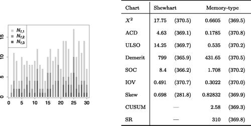
In this section, we demonstrate the application of the control charts studied in Section 4 by means of a real-data example. We use a data set from manufacturing industry that was presented by Li, Tsung, and Zou (2014), and where the corresponding in-control model was taken as an inspiration for the (high-quality) Scenario 4 in Section 4. Now, let us focus on the Phase-II data for illustration.

The data set consists of 30 samples with a unique sample size of n = 64, where each individual observation expresses the quality of a manufactured electric toothbrush head. Here, the quality is measured in terms of the excess plastic (known as “flash”), which may arise on the brush head when its two components are welded together. The extent of flash is classified into the $d+1=4$ ordinal categories $s_0=“\text{slight}\mathrm{”},{\mathrm{s}}_1=\mathrm{“}\text{small}\mathrm{”},{\mathrm{s}}_2=\mathrm{“}\text{medium}\mathrm{”},$ and $s_3=“\text{large}\mathrm{”}.$ These categories are ordered according to degrading quality, because increasing flash implies a higher risk of injury. Figure 1 (left) shows the sample frequencies $N_{t,1},N_{t,2},N_{t,3}$ (corresponding to non-optimal quality) as a bar plot, whereas the absolute frequencies $N_{t,0},$ referring to the best quality, result from the difference $n-N_{t,1}-N_{t,2}-N_{t,3}.$ On the right-hand side of Figure 1, the control limits of the charts and their corresponding in-control ARLs are displayed, which are again determined by simulations with 10⁶ replications. This time, the chart designs are based on the exact in-control PMF ${\mathit{p}}_0=(0.8631,0.0804,0.0357,0.0208)$ as given in Li, Tsung, and Zou (2014) (not on the “smoothed” version used for Scenario 4). Like in Section 4, the Shewhart version of the skew chart is the most inflexible in adjusting its ARL₀ to the target value of 370.

Despite its low ARL₀, the skew chart triggers an alarm only at time t = 25, just like the other Shewhart-type charts do, see Figure D.1 in Appendix D. In fact, the 25th sample causing the alarm expresses the worst quality among all samples, see Figure 1 (left): the total frequency $N_{t,1}+N_{t,2}+N_{t,3}$ of non-optimal quality as well as the frequency $N_{t,3}$ of worst quality are maximal for t = 25. However, due to their lack of memory, the Shewhart charts of Figure D.1 do not indicate that there seems to be some disturbing trend already before t = 25 (such a trend is also hardly visible from Figure 1). This trend gets clear from the memory-type charts in Figure D.2, i.e., if EWMA-smoothing with $\lambda =0.1$ is added to the aforementioned charts, or if CUSUM and SR charts are considered (defining ${\mathit{p}}_1$ by a logit model with location shift 0.1). The statistics of all memory charts start to gradually increase (or decrease in the case of the skew chart) around t = 20. But unlike the Shewhart charts, only three memory charts, namely demerit, IOV, and skew, signal a change already at t = 25. The remaining memory charts trigger their first alarm with a delay between one and four samples. This illustrates the well-known dilemma of memory-type charts: they are able to detect a gradual deterioration or small shift in the process, but they may be slow in recognizing a sudden large shift (such as for t = 25). Shewhart charts, by contrast, typically show the opposite performance and are, thus, uniquely successful in the present data example. It is therefore all the more remarkable that the EWMA versions of the demerit, IOV, and skew chart are as quick as their Shewhart versions. This outstanding performance of the demerit and skew charts is consistent with our general findings in Section 4, and for the IOV chart, it follows from the fact that we are concerned with a high-quality situation (i.e., maximal in-control probability for the best quality level).

Figure 1. Left: Frequencies $N_{t,1},N_{t,2},N_{t,3}$ of flash types $s_1,s_2,s_3$ on toothbrush heads, where $N_{t,0}=64-N_{t,1}-N_{t,2}-N_{t,3}.$ Right: Control limits of considered control charts, simulated ARL₀ in parentheses.

6. Conclusions and future research

In this paper, we provided an extensive survey of sample-based control charts for monitoring i.i.d. univariate ordinal data. The control charts in the literature were classified into identified groups of control statistics for comparisons and discussions. Some new results and proposals were given to supplement the existing work. A simulation study of the discussed control charts was completed for evaluating and comparing the performance under four diverse in-control scenarios. These four scenarios were inspired by real-world applications from the literature, and they were embedded into common parametric models for ordinal data to get a variety of out-of-control scenarios. Our simulation results indicate that demerit-type charts perform considerably well for monitoring ordinal medium-quality observations, with little influence from the actual weighting scheme. For the high-quality setting scenarios, again the demerit-type charts are among the best performing charts, with the IOV chart being a strong competitor. In conclusion, the demerit principle proves to be very effective in process monitoring applications with ordinal data, and a demerit-type chart (including the skew chart) in combination with the EWMA smoothing is recommended based on the cases studied.

There are several directions for future research on control charts for ordinal processes. First, ordinal control charts for individual observations (rather than samples taken from the process) should be developed. This would not only be relevant for automated production processes with 100% inspection, but also for a second future research direction, the monitoring of ordinal time series data. We conjecture that serial dependence between individual observations (or within samples taken from the process) will impact the performance of control charts being developed for i.i.d. data, such that a revised chart design or novel types of control charts are necessary in such a case. To our knowledge, Li, Xu, and Zhou (2018); Li and Lu (2022) are the only proposals on sequential methods for ordinal time series up to now. More articles are available on the monitoring of multivariate ordinal data, see Wang, Li, and Su (2017); Bai and Li (2021); Hakimi et al. (2021) and the references therein, but an extensive comparative study is yet missing. Finally, as real-world ordinal time series often exhibit missing data, see Weiß (2021b), it would be interesting to discuss how control charts should be adapted to account for missingness.

Acknowledgments

The authors thank the two referees for their useful comments on an earlier draft of this article. The authors are grateful to Professor Jian Li (Xi’an Jiaotong University, China) for providing the flash data discussed in Section 5.

Data availability statement

The data that support the findings of this study are available from the corresponding author, C.H. Weiß, upon reasonable request.

Disclosure statement

The authors report no conflict of interest.

Additional information

Funding

This work was supported by the Interne Forschungsförderung 2021 (IFF 2021) of Helmut Schmidt University.

Notes

1 Another type of qualitative data, which is not considered here, are nominal data, where we do not have such a natural order; corresponding SPC references can be found in Weiß (2021a).

Appendix A.

Tabulated ARL results of Section 4

Table A.1. Scenario 1: ARL performance of control charts [3.1[3.1] $${\mathrm{X}}_t^2=\sum _{j=0}^d\frac{{(N_{t,j}-n p_{0,j})}^2}{n p_{0,j}}=n^{-1} {({\mathit{N}}_t-n {\mathit{p}}_0)}^{\top } \mathrm{ }\text{diag}{({\mathit{p}}_0)}^{-1} ({\mathit{N}}_t-n {\mathit{p}}_0).$$[3.1] ] to [3.11[3.11] $${\text{skew}}_t=(\frac{2}{d} \sum _{j=0}^{d-1}{\widehat{f}}_{t,j})-1,$$[3.11] ].

	Chart	X^2	ACD	ULSO	Demerit	SOC	IOV	Skew	CUSUM	SR
	CL	13.05	2.204		397	11	0.447	−0.109
Shewhart	ARL0	365.4	365.4		367.4	316.2	371.2	288.5
1-IB, $\pi =$	0.51	339.0	326.6		237.6	283.3	371.6	182.9
	0.52	275.9	244.5		157.1	212.4	371.4	118.4
	0.53	207.3	168.5		106.3	146.6	370.4	78.2
	0.54	149.3	113.3		73.4	98.9	370.6	52.9
	0.55	106.1	76.5		51.9	66.9	370.3	36.7
	0.56	75.5	52.5		37.1	45.8	369.1	26.0
	0.57	54.2	36.7		27.2	32.2	368.0	18.8
	0.58	39.4	26.2		20.3	23.0	365.1	13.9
N $(\mu ,1),\mu =$	0.03	314.1	293.9		198.5	255.4	368.2	151.8
	0.06	215.0	178.9		112.2	155.7	362.1	83.4
	0.09	133.4	101.2		65.6	88.4	351.5	47.8
	0.12	80.7	57.9		39.9	50.9	336.5	28.7
	0.15	49.4	34.3		25.2	30.4	318.0	17.9
	0.18	31.0	21.3		16.4	18.9	295.1	11.7
	0.21	20.0	13.7		11.1	12.3	270.2	7.9
	0.24	13.3	9.2		7.8	8.3	242.2	5.6
Log $(\mu ,1),\mu =$	0.05	329.5	314.5		221.4	272.6	368.6	170.1
	0.10	249.7	217.4		136.9	189.1	362.2	103.1
	0.15	172.2	137.3		86.7	120.2	350.7	64.1
	0.20	113.9	85.6		56.1	75.2	334.9	41.1
	0.25	75.0	54.3		37.2	47.8	316.1	27.1
	0.30	49.6	35.1		25.3	31.2	294.5	18.4
	0.35	33.3	23.4		17.6	20.9	270.3	12.8
	0.40	22.8	16.0		12.5	14.4	244.4	9.2
	CL	0.53	0.091		348.62	2.222	0.3112	−0.02136	2.006	333
EWMA	ARL0	365.7	373.0		370.6	370.3	373.4	370.6	370.7	370.0
1-IB, $\pi =$	0.51	201.4	170.7		118.6	169.0	369.3	104.8	95.3	112.3
	0.52	81.5	64.3		52.2	63.5	358.8	44.0	45.9	64.8
	0.53	40.3	32.4		29.0	32.0	342.9	24.3	29.4	46.5
	0.54	24.3	20.1		18.9	19.9	320.6	15.9	21.6	36.7
	0.55	16.9	14.2		13.7	14.1	295.7	11.7	17.0	30.6
	0.56	12.8	10.9		10.6	10.8	267.5	9.1	14.1	26.3
	0.57	10.2	8.9		8.6	8.7	238.6	7.5	12.0	23.1
	0.58	8.6	7.5		7.3	7.4	210.2	6.4	10.5	20.7
N $(\mu ,1),\mu =$	0.03	136.1	109.9		81.0	108.6	359.7	70.0	66.8	85.7
	0.06	44.5	35.6		31.2	35.2	323.5	26.4	31.3	48.7
	0.09	21.9	18.2		17.0	18.0	272.0	14.6	20.2	34.9
	0.12	13.8	11.8		11.2	11.7	216.3	9.8	14.9	27.5
	0.15	10.0	8.7		8.3	8.6	164.2	7.4	11.8	22.9
	0.18	7.8	6.9		6.5	6.8	120.3	5.9	9.8	19.6
	0.21	6.4	5.7		5.3	5.6	86.3	4.9	8.4	17.3
	0.24	5.5	4.9		4.5	4.8	61.6	4.2	7.3	15.4
Log $(\mu ,1),\mu =$	0.05	174.0	144.0		101.7	142.4	361.9	89.4	82.6	100.5
	0.10	63.4	50.2		41.8	49.6	330.3	35.6	39.1	57.6
	0.15	30.8	25.2		22.8	24.9	284.2	19.5	25.1	41.2
	0.20	18.9	15.9		14.8	15.7	232.5	12.9	18.4	32.5
	0.25	13.3	11.4		10.7	11.3	182.9	9.5	14.5	27.0
	0.30	10.2	8.8		8.3	8.8	138.8	7.5	12.0	23.1
	0.35	8.2	7.2		6.8	7.1	103.1	6.2	10.2	20.3
	0.40	6.9	6.1		5.7	6.0	75.4	5.3	8.9	18.1

Note: ARLs of ULSO chart omitted as these are identical to those of X² in Scenario 1.

Table A.2. Scenario 2: ARL performance of control charts [3.1[3.1] $${\mathrm{X}}_t^2=\sum _{j=0}^d\frac{{(N_{t,j}-n p_{0,j})}^2}{n p_{0,j}}=n^{-1} {({\mathit{N}}_t-n {\mathit{p}}_0)}^{\top } \mathrm{ }\text{diag}{({\mathit{p}}_0)}^{-1} ({\mathit{N}}_t-n {\mathit{p}}_0).$$[3.1] ] to [3.11[3.11] $${\text{skew}}_t=(\frac{2}{d} \sum _{j=0}^{d-1}{\widehat{f}}_{t,j})-1,$$[3.11] ].

	Chart	X^2	ACD	ULSO	Demerit	SOC	IOV	Skew	CUSUM	SR
	CL	15.285	4.7	12.66	4993	13.195	0.19	−0.3066
Shewhart	ARL0	374.0	371.4	369.3	375.6	370.8	382.0	309.4
2-IB, $\pi =$	0.51	358.0	474.2	308.8	205.0	368.4	297.4	171.8
	0.52	281.8	422.9	220.8	115.9	264.8	234.6	98.6
	0.53	195.4	282.9	146.1	67.6	162.0	187.8	58.4
	0.54	127.9	168.8	94.2	41.0	95.7	152.4	35.7
	0.55	82.1	98.8	60.5	25.6	57.2	125.1	22.6
	0.56	53.1	59.0	39.3	16.6	35.0	103.6	14.8
	0.57	34.6	36.2	26.0	11.2	22.2	87.4	10.0
	0.58	23.1	22.9	17.5	7.7	14.5	74.5	7.0
N $(\mu ,1),\mu =$	0.03	365.3	478.2	302.5	183.6	355.2	263.1	153.4
	0.06	276.7	362.3	201.2	94.4	218.9	187.3	80.2
	0.09	181.0	204.4	123.2	51.2	117.6	137.1	44.4
	0.12	111.4	109.2	73.8	29.3	63.5	103.7	25.7
	0.15	67.5	59.8	44.7	17.6	35.8	80.5	15.7
	0.18	41.5	34.3	27.7	11.1	21.2	64.0	10.1
	0.21	26.1	20.6	17.6	7.4	13.2	52.4	6.7
	0.24	16.9	12.9	11.6	5.1	8.6	43.8	4.8
Log $(\mu ,1),\mu =$	0.05	382.5	478.0	323.0	201.7	370.9	263.1	168.2
	0.10	321.9	402.7	236.2	112.7	254.7	187.4	95.1
	0.15	237.3	255.1	158.3	65.5	150.0	137.7	56.2
	0.20	162.2	148.8	103.3	39.7	86.9	103.3	34.6
	0.25	107.6	87.0	66.8	25.0	51.7	79.7	22.1
	0.30	70.5	52.4	43.5	16.4	32.0	63.1	14.7
	0.35	46.7	32.7	28.9	11.1	20.5	51.1	10.1
	0.40	31.3	21.2	19.6	7.8	13.6	42.2	7.2
	CL	0.653	0.1974	0.531	4521.9	2.712	0.31037	−0.22175	2.257	327
EWMA	ARL0	371.3	370.0	369.6	371.9	369.9	371.3	370.1	370.1	370.6
2-IB, $\pi =$	0.51	173.3	143.5	155.6	79.5	133.5	171.6	77.7	76.2	89.0
	0.52	58.3	47.0	54.0	30.5	44.2	93.2	29.8	34.8	48.7
	0.53	27.5	23.2	26.2	16.6	22.0	57.8	16.4	22.0	34.1
	0.54	16.8	14.6	16.2	11.0	13.9	39.8	10.9	16.0	26.6
	0.55	11.9	10.5	11.5	8.2	10.0	29.6	8.1	12.6	21.9
	0.56	9.2	8.2	8.8	6.5	7.8	23.4	6.5	10.4	18.7
	0.57	7.5	6.7	7.2	5.4	6.4	19.3	5.4	8.8	16.4
	0.58	6.3	5.7	6.1	4.6	5.4	16.6	4.6	7.7	14.6
N $(\mu ,1),\mu =$	0.03	142.8	104.3	118.3	61.3	96.6	130.5	61.2	59.4	73.2
	0.06	43.8	32.4	37.4	22.6	30.3	62.5	22.8	27.2	40.2
	0.09	21.1	16.7	18.7	12.7	15.7	37.0	12.8	17.5	28.5
	0.12	13.4	10.9	12.1	8.6	10.4	25.5	8.7	12.9	22.4
	0.15	9.7	8.1	8.9	6.5	7.7	19.3	6.7	10.3	18.6
	0.18	7.7	6.5	7.0	5.3	6.2	15.7	5.4	8.5	15.9
	0.21	6.4	5.5	5.8	4.4	5.2	13.4	4.6	7.3	14.0
	0.24	5.4	4.7	5.0	3.9	4.5	11.8	4.0	6.4	12.6
Log $(\mu ,1),\mu =$	0.05	170.3	123.6	139.6	72.0	114.2	135.4	73.1	67.2	80.5
	0.10	56.2	39.8	46.3	27.4	37.0	65.5	28.0	30.9	44.4
	0.15	26.8	20.2	22.9	15.2	18.9	39.0	15.6	19.8	31.5
	0.20	16.5	13.0	14.5	10.3	12.3	26.6	10.6	14.6	24.7
	0.25	11.9	9.6	10.6	7.7	9.1	20.1	8.0	11.7	20.6
	0.30	9.3	7.6	8.3	6.2	7.2	16.2	6.4	9.7	17.7
	0.35	7.6	6.4	6.9	5.2	6.0	13.7	5.4	8.3	15.7
	0.40	6.5	5.5	5.9	4.5	5.2	12.0	4.7	7.3	14.1

Table A.3. Scenario 3: ARL performance of control charts [3.1[3.1] $${\mathrm{X}}_t^2=\sum _{j=0}^d\frac{{(N_{t,j}-n p_{0,j})}^2}{n p_{0,j}}=n^{-1} {({\mathit{N}}_t-n {\mathit{p}}_0)}^{\top } \mathrm{ }\text{diag}{({\mathit{p}}_0)}^{-1} ({\mathit{N}}_t-n {\mathit{p}}_0).$$[3.1] ] to [3.11[3.11] $${\text{skew}}_t=(\frac{2}{d} \sum _{j=0}^{d-1}{\widehat{f}}_{t,j})-1,$$[3.11] ].

	Chart	X^2	ACD	ULSO	Demerit	SOC	IOV	Skew	CUSUM	SR
	CL	20.35	9.67	12.337	505	15.62	0.5731	0.505
Shewhart	ARL0	370.5	370.4	371.9	363.3	372.1	369.8	384.9
0-IB, $\pi =$	0.31	214.5	214.8	193.9	151.1	250.6	156.9	167.1
	0.32	122.2	108.9	96.2	69.4	142.3	72.8	79.4
	0.33	69.5	56.9	49.1	34.8	80.1	36.7	41.0
	0.34	40.4	31.5	26.4	19.1	46.8	20.0	22.9
	0.35	24.0	18.6	15.1	11.3	28.8	11.7	13.7
	0.36	14.8	11.7	9.2	7.2	18.7	7.4	8.8
	0.37	9.6	7.8	6.0	4.9	12.7	4.9	6.0
	0.38	6.4	5.4	4.1	3.5	9.0	3.5	4.3
N $(\mu ,1),\mu =$	0.03	249.0	218.1	227.3	169.9	238.2	198.6	172.6
	0.06	160.6	108.8	127.5	84.3	121.7	111.5	82.7
	0.09	101.7	55.1	70.6	44.3	61.6	65.2	42.3
	0.12	63.6	29.4	39.7	24.7	32.8	39.9	23.1
	0.15	39.5	16.7	23.1	14.6	18.5	25.4	13.4
	0.18	24.9	10.1	14.0	9.1	11.0	16.8	8.3
	0.21	16.0	6.5	8.9	6.0	7.0	11.6	5.4
	0.24	10.5	4.4	5.9	4.1	4.7	8.3	3.8
Log $(\mu ,1),\mu =$	0.04	295.2	252.1	268.8	208.4	269.1	246.2	208.2
	0.08	226.2	148.3	177.7	123.3	160.8	166.7	117.0
	0.12	167.6	85.5	113.9	75.0	92.2	115.1	68.1
	0.16	121.3	50.5	72.1	47.0	53.8	81.1	41.1
	0.20	86.0	30.8	46.1	30.1	32.5	57.9	25.7
	0.24	60.0	19.5	29.9	20.0	20.4	42.5	16.6
	0.28	41.6	12.8	19.7	13.6	13.3	31.6	11.2
	0.32	28.9	8.7	13.4	9.6	9.0	23.9	7.7
	CL	0.7759	0.4155	0.532	404.32	3.238	0.4886	0.6143	2.205	327.6
EWMA	ARL0	370.2	370.9	372.5	369.7	369.2	372.1	369.9	370.4	370.8
0-IB, $\pi =$	0.31	98.4	84.4	84.8	51.5	101.7	51.0	55.5	64.9	79.6
	0.32	31.7	27.4	26.7	18.9	34.0	18.5	20.6	30.2	44.4
	0.33	16.2	14.5	13.9	10.7	17.9	10.4	11.6	19.5	31.6
	0.34	10.6	9.6	9.2	7.3	11.8	7.1	8.0	14.5	25.0
	0.35	7.8	7.2	6.9	5.6	8.8	5.4	6.1	11.6	20.8
	0.36	6.2	5.8	5.5	4.5	7.0	4.3	5.0	9.7	18.0
	0.37	5.2	4.9	4.5	3.8	5.9	3.6	4.2	8.3	15.9
	0.38	4.4	4.2	3.9	3.3	5.1	3.2	3.6	7.4	14.3
N $(\mu ,1),\mu =$	0.03	115.2	80.1	97.3	59.1	81.7	70.6	55.5	55.0	69.9
	0.06	37.3	25.5	30.5	21.6	25.8	26.4	20.2	25.1	38.4
	0.09	18.6	13.4	15.6	11.9	13.6	14.4	11.2	16.1	27.1
	0.12	11.9	8.9	10.2	8.1	9.0	9.6	7.7	11.8	21.2
	0.15	8.7	6.7	7.5	6.1	6.7	7.1	5.8	9.3	17.5
	0.18	6.9	5.3	6.0	4.9	5.4	5.6	4.7	7.7	14.9
	0.21	5.7	4.4	5.0	4.1	4.5	4.6	3.9	6.6	13.1
	0.24	4.9	3.8	4.3	3.5	3.9	3.9	3.4	5.8	11.6
Log $(\mu ,1),\mu =$	0.04	160.4	113.1	136.0	85.7	112.4	106.3	77.3	69.7	84.0
	0.08	58.3	37.6	46.0	33.5	37.2	44.4	29.5	32.0	46.3
	0.12	28.2	19.2	22.8	18.3	18.9	24.3	16.2	20.3	32.6
	0.16	17.3	12.3	14.4	12.0	12.2	15.8	10.7	14.9	25.5
	0.20	12.3	9.0	10.4	8.8	8.9	11.4	8.0	11.7	21.0
	0.24	9.5	7.1	8.1	7.0	7.0	8.8	6.3	9.7	18.0
	0.28	7.7	5.8	6.6	5.7	5.8	7.2	5.2	8.2	15.7
	0.32	6.5	5.0	5.6	4.9	4.9	6.0	4.5	7.2	14.0

Table A.4. Scenario 4: ARL performance of control charts [3.1[3.1] $${\mathrm{X}}_t^2=\sum _{j=0}^d\frac{{(N_{t,j}-n p_{0,j})}^2}{n p_{0,j}}=n^{-1} {({\mathit{N}}_t-n {\mathit{p}}_0)}^{\top } \mathrm{ }\text{diag}{({\mathit{p}}_0)}^{-1} ({\mathit{N}}_t-n {\mathit{p}}_0).$$[3.1] ] to [3.11[3.11] $${\text{skew}}_t=(\frac{2}{d} \sum _{j=0}^{d-1}{\widehat{f}}_{t,j})-1,$$[3.11] ].

	Chart	X^2	ACD	ULSO	Demerit	SOC	IOV	Skew	CUSUM	SR
	CL	17.735	4.83	13.57	1089	11.004	0.4573	0.72
Shewhart	ARL0	367.4	369.5	371.5	368.3	370.4	366.4	338.7
0-IB, $\pi =$	0.42	190.6	200.0	187.5	164.3	249.4	173.4	170.0
	0.44	100.9	113.1	95.4	80.1	170.3	89.4	92.3
	0.46	55.7	67.2	50.6	42.6	119.1	49.8	53.6
	0.48	32.1	42.0	28.3	24.4	86.2	29.8	33.1
	0.50	19.4	27.5	16.7	15.0	64.1	18.9	21.6
	0.52	12.3	18.8	10.5	9.8	49.2	12.7	14.8
	0.54	8.2	13.4	6.9	6.7	38.8	9.0	10.5
	0.56	5.7	9.9	4.8	4.9	31.5	6.6	7.8
N $(\mu ,1),\mu =$	0.03	233.1	199.8	223.0	207.2	206.6	195.0	177.5
	0.06	148.4	109.0	133.9	120.0	113.6	108.0	97.1
	0.09	94.5	61.6	81.1	71.6	64.0	62.2	55.3
	0.12	60.5	36.1	49.9	43.9	37.7	37.1	32.7
	0.15	39.0	22.1	31.2	27.9	23.0	23.1	20.3
	0.18	25.7	14.1	20.1	18.3	14.7	14.9	13.0
	0.21	17.1	9.4	13.3	12.4	9.7	10.0	8.7
	0.24	11.7	6.5	9.1	8.6	6.7	6.9	6.1
Log $(\mu ,1),\mu =$	0.05	259.8	217.4	246.5	235.2	218.5	218.1	195.8
	0.10	180.6	127.7	160.6	151.8	126.4	132.9	116.7
	0.15	123.9	76.6	103.6	99.5	74.3	82.9	70.9
	0.20	84.1	47.0	66.8	66.0	44.9	52.8	44.3
	0.25	56.7	29.7	43.3	44.7	28.0	34.4	28.5
	0.30	38.3	19.4	28.5	30.7	18.0	23.0	18.8
	0.35	26.0	13.0	19.0	21.5	12.0	15.7	12.8
	0.40	17.8	9.0	13.0	15.3	8.3	11.1	8.9
	CL	0.66	0.1967	0.5345	677.1	2.263	0.31575	0.81686	2.96	296
EWMA	ARL0	374.6	366.9	372.8	370.5	371.9	367.8	371.4	371.5	371.3
0-IB, $\pi =$	0.42	103.3	116.7	96.6	64.0	176.4	73.8	79.1	117.3	115.1
	0.44	34.7	42.2	32.0	24.0	76.9	28.8	31.3	55.5	59.2
	0.46	17.7	22.1	16.4	13.3	42.2	16.1	17.5	34.1	39.5
	0.48	11.3	14.3	10.6	9.0	27.5	10.9	11.8	24.4	30.1
	0.50	8.2	10.5	7.7	6.7	20.2	8.1	8.8	19.1	24.6
	0.52	6.4	8.2	6.0	5.4	15.9	6.5	7.1	15.8	21.1
	0.54	5.3	6.8	4.9	4.5	13.1	5.4	5.9	13.6	18.6
	0.56	4.4	5.8	4.1	3.8	11.3	4.7	5.1	12.0	16.8
N $(\mu ,1),\mu =$	0.03	131.0	105.5	122.0	90.3	109.3	78.7	77.3	75.2	76.7
	0.06	47.6	36.1	42.9	35.6	36.9	30.0	29.3	30.8	36.3
	0.09	23.8	18.5	21.5	19.2	18.9	16.3	15.9	18.3	23.7
	0.12	14.9	11.9	13.6	12.4	12.1	10.7	10.5	12.8	17.7
	0.15	10.6	8.6	9.7	9.0	8.7	7.8	7.7	9.8	14.1
	0.18	8.2	6.7	7.5	7.0	6.8	6.1	6.0	7.9	11.8
	0.21	6.6	5.5	6.1	5.7	5.6	5.0	5.0	6.6	10.1
	0.24	5.6	4.6	5.2	4.8	4.7	4.3	4.2	5.7	8.8
Log $(\mu ,1),\mu =$	0.05	151.9	125.8	141.7	114.8	123.6	95.5	92.7	84.0	84.8
	0.10	58.1	44.9	52.1	48.9	43.1	38.4	36.7	34.9	40.2
	0.15	28.8	22.7	25.9	26.6	21.8	20.7	19.8	20.5	26.0
	0.20	17.7	14.3	16.0	17.1	13.7	13.4	12.8	14.2	19.3
	0.25	12.4	10.2	11.3	12.2	9.8	9.7	9.3	10.8	15.3
	0.30	9.5	7.8	8.7	9.3	7.6	7.5	7.2	8.7	12.8
	0.35	7.6	6.3	7.0	7.5	6.1	6.1	5.9	7.2	10.9
	0.40	6.3	5.3	5.9	6.2	5.2	5.1	4.9	6.2	9.5

Table A.5. In-control and out-of-control PMFs for Scenarios 1–4.

Scenario 1		Scenario 2		Scenario 3		Scenario 4
${\mathit{p}}_0$	(0.075,0.850,0.075)	${\mathit{p}}_0$	(0.050,0.150,0.750,0.050)	${\mathit{p}}_0$	(0.544,0.247,0.159,0.045,0.005)	${\mathit{p}}_0$	(0.843,0.086,0.058,0.013)
1-IB $\pi =$ 0.51	(0.072,0.850,0.078)	2-IB $\pi =$ 0.51	(0.047,0.147,0.753,0.053)	0-IB $\pi =$ 0.31	(0.536,0.244,0.165,0.049,0.006)	0-IB $\pi =$ 0.42	(0.839,0.085,0.061,0.015)
0.52	(0.069,0.850,0.081)	0.52	(0.044,0.144,0.756,0.056)	0.32	(0.528,0.241,0.170,0.053,0.006)	0.44	(0.835,0.083,0.065,0.017)
0.53	(0.066,0.849,0.084)	0.53	(0.042,0.140,0.758,0.060)	0.33	(0.521,0.238,0.176,0.058,0.007)	0.46	(0.831,0.080,0.069,0.019)
0.54	(0.063,0.849,0.087)	0.54	(0.039,0.137,0.761,0.063)	0.34	(0.514,0.235,0.181,0.062,0.008)	0.48	(0.828,0.078,0.072,0.022)
0.55	(0.061,0.849,0.091)	0.55	(0.036,0.134,0.763,0.067)	0.35	(0.507,0.231,0.186,0.067,0.009)	0.50	(0.825,0.075,0.075,0.025)
0.56	(0.058,0.848,0.094)	0.56	(0.034,0.130,0.766,0.070)	0.36	(0.501,0.226,0.191,0.072,0.010)	0.52	(0.822,0.072,0.078,0.028)
0.57	(0.055,0.847,0.097)	0.57	(0.032,0.126,0.768,0.074)	0.37	(0.495,0.222,0.196,0.077,0.011)	0.54	(0.819,0.069,0.080,0.031)
0.58	(0.053,0.846,0.101)	0.58	(0.030,0.123,0.770,0.078)	0.38	(0.489,0.217,0.200,0.082,0.013)	0.56	(0.817,0.065,0.083,0.035)
N $\mu =$ 0.03	(0.071,0.850,0.079)	N $\mu =$ 0.03	(0.047,0.145,0.755,0.053)	N $\mu =$ 0.03	(0.532,0.250,0.164,0.048,0.005)	N $\mu =$ 0.03	(0.836,0.090,0.061,0.014)
0.06	(0.067,0.849,0.084)	0.06	(0.044,0.140,0.760,0.056)	0.06	(0.520,0.253,0.170,0.051,0.006)	0.06	(0.828,0.093,0.064,0.015)
0.09	(0.063,0.848,0.089)	0.09	(0.041,0.134,0.764,0.060)	0.09	(0.508,0.256,0.176,0.054,0.006)	0.09	(0.821,0.096,0.067,0.016)
0.12	(0.059,0.847,0.093)	0.12	(0.039,0.129,0.768,0.064)	0.12	(0.496,0.259,0.181,0.057,0.007)	0.12	(0.813,0.099,0.071,0.017)
0.15	(0.056,0.845,0.099)	0.15	(0.036,0.124,0.772,0.067)	0.15	(0.484,0.261,0.187,0.060,0.007)	0.15	(0.804,0.103,0.074,0.019)
0.18	(0.053,0.843,0.104)	0.18	(0.034,0.119,0.775,0.071)	0.18	(0.472,0.263,0.193,0.064,0.008)	0.18	(0.796,0.106,0.078,0.020)
0.21	(0.050,0.841,0.109)	0.21	(0.032,0.115,0.778,0.076)	0.21	(0.460,0.265,0.198,0.067,0.009)	0.21	(0.787,0.109,0.082,0.022)
0.24	(0.047,0.838,0.115)	0.24	(0.030,0.110,0.780,0.080)	0.24	(0.449,0.267,0.204,0.071,0.009)	0.24	(0.779,0.113,0.086,0.023)
Log $\mu =$ 0.05	(0.072,0.850,0.079)	Log $\mu =$ 0.05	(0.048,0.144,0.755,0.052)	Log $\mu =$ 0.04	(0.534,0.250,0.164,0.047,0.005)	Log $\mu =$ 0.05	(0.836,0.090,0.060,0.013)
0.10	(0.068,0.849,0.082)	0.10	(0.045,0.139,0.761,0.055)	0.08	(0.524,0.253,0.168,0.049,0.005)	0.10	(0.830,0.093,0.063,0.014)
0.15	(0.065,0.849,0.086)	0.15	(0.043,0.134,0.765,0.058)	0.12	(0.514,0.256,0.173,0.051,0.005)	0.15	(0.822,0.097,0.066,0.015)
0.20	(0.062,0.848,0.090)	0.20	(0.041,0.129,0.770,0.060)	0.16	(0.504,0.259,0.178,0.053,0.006)	0.20	(0.815,0.100,0.069,0.016)
0.25	(0.059,0.846,0.094)	0.25	(0.039,0.124,0.774,0.063)	0.20	(0.494,0.262,0.183,0.055,0.006)	0.25	(0.807,0.104,0.072,0.016)
0.30	(0.057,0.845,0.099)	0.30	(0.038,0.119,0.777,0.066)	0.24	(0.484,0.264,0.188,0.057,0.006)	0.30	(0.799,0.108,0.076,0.017)
0.35	(0.054,0.843,0.103)	0.35	(0.036,0.114,0.781,0.069)	0.28	(0.474,0.267,0.194,0.059,0.006)	0.35	(0.791,0.112,0.079,0.018)
0.40	(0.052,0.841,0.108)	0.40	(0.034,0.109,0.784,0.073)	0.32	(0.464,0.269,0.199,0.061,0.007)	0.40	(0.783,0.116,0.083,0.019)

Appendix B.

On a CDF-based Pearson-type GoF-Statistic

Let X be an ordinal random variable with PMF p such that $p_j>0$ for all $j=0,\dots ,d$ (otherwise, the range $\mathcal{S}$ could be reduced by removing the categories with probability zero); as before, let f be the corresponding CDF. If the sample CDF $\widehat{\mathit{f}}$ is computed from n i.i.d. replicates of X, then its asymptotic distribution is known from (Kiesl 2003, p. 99): we have $\sqrt{n} (\widehat{\mathit{f}}-\mathit{f})\stackrel{\mathrm{d}}{\to }\mathrm{N}(\mathbf{0},\mathbf{\Sigma }),$ where the covariance matrix $\mathbf{\Sigma }={({\sigma }_{i,j})}_{i,j=0,\dots ,d-1}$ has the entries ${\sigma }_{i,j} = f_{\min \{i,j\}}-f_i f_j.$ Thus, a Pearson-type GoF-statistic based on the sample CDF, as well as its asymptotic distribution, are immediately implied as (B.1) $${\tilde{\mathrm{X}}}^2=n {(\widehat{\mathit{f}}-\mathit{f})}^{\top } {\mathbf{\Sigma }}^{-1} (\widehat{\mathit{f}}-\mathit{f})\hspace{1em}\stackrel{\mathrm{d}}{\to }{\chi }_d^2,$$(B.1) provided that ${\mathbf{\Sigma }}^{-1}$ exists. In what follows, we show that this CDF-based statistic ${\tilde{\mathrm{X}}}^2$ is indeed identical to the ordinary Pearson statistic ${\mathrm{X}}^2$ from (3.1).

Lemma B.1.

If $p_j>0$ for all $j=0,\dots ,d$, then the inverse matrix ${\mathbf{\Sigma }}^{-1}={(s_{ij})}_{i,j=0,\dots ,d-1}$ exists and is symmetric, i.e., s_ij = s_ji. Its entries s_ij for $j\ge i$ are given by$$s_{ij}=\{\begin{array}{cc}\frac{1}{p_i}+\frac{1}{p_{i+1}}\hfill & \mathit{\text{if}}\mathrm{ }j=i\in \{0,\dots ,d-1\},\hfill \\ -\frac{1}{p_{i+1}}\hfill & \mathit{\text{if}}\mathrm{ }j=i+1\in \{1,\dots ,d-1\},\hfill \\ 0\hfill & \text{otherwise}.\hfill \end{array}$$

Here, it is understood that ${\mathbf{\Sigma }}^{-1}=\frac{1}{p_0}+\frac{1}{p_1}\in (1;\infty )$ if d = 1.

Note that ${\mathbf{\Sigma }}^{-1}$ is a (symmetric) tridiagonal matrix according to Lemma B.1.

Proof.

We prove Lemma B.1 by showing that the given expression for ${\mathbf{\Sigma }}^{-1}$ satisfies $\mathbf{\Sigma } {\mathbf{\Sigma }}^{-1}=\mathbf{I},$ where I denotes the d × d-identity matrix. If d = 1, then $${\sigma }_{00} s_{00}=f_0 (1-f_0) (\frac{1}{p_0}+\frac{1}{p_1})=p_0 p_1 \frac{p_1+p_0}{p_0 p_1}=1.$$

If d = 2, then $$\begin{array}{c}\mathbf{\Sigma } {\mathbf{\Sigma }}^{-1}=\left(\begin{array}{cc}{f}_0 (1-f_0)& f_0 (1-f_1)\\ f_0 (1-f_1)& f_1 (1-f_1)\end{array}\right)\left(\begin{array}{cc}\frac{1}{p_0}+\frac{1}{p_1}& -\frac{1}{p_1}\\ -\frac{1}{p_1}& \frac{1}{p_1}+\frac{1}{p_2}\end{array}\right)\\ =\left(\begin{array}{cc}\frac{f_0 (1-f_0)}{p_0}+\frac{f_0 (f_1-f_0)}{p_1}& \frac{f_0 (1-f_1)}{p_2}+\frac{f_0 (f_0-f_1)}{p_1}\\ \frac{f_0 (1-f_1)}{p_0}+\frac{(f_0-f_1) (1-f_1)}{p_1}& \frac{f_1 (1-f_1)}{p_2}+\frac{(f_1-f_0) (1-f_1)}{p_1}\end{array}\right)\\ =\left(\begin{array}{cc}(1-f_0)+f_0& f_0-f_0\\ (1-f_1)-(1-f_1)& f_1+(1-f_1)\end{array}\right)=\left(\begin{array}{cc}1& 0\\ 0& 1\end{array}\right).\end{array}$$

For $d\ge 3,$ the entries of $\mathbf{\Sigma } {\mathbf{\Sigma }}^{-1},$ namely ${\sum }_{k=0}^{d-1}{\sigma }_{ik} s_{kj}$ for $i,j\in \{0,\dots ,d-1\},$ consist of at most three summands because of the tridiagonal structure of ${\mathbf{\Sigma }}^{-1}.$ This happens if $1\le j\le d-2,$ whereas $j\in \{0,d-1\}$ leads to two summands of the same structure as in the case d = 2. Thus, let us focus on $1\le j\le d-2:$ $$\begin{array}{c}\sum _{k=0}^{d-1}{\sigma }_{ik} s_{kj}={\sigma }_{i,j-1} s_{j-1,j}+{\sigma }_{ij} s_{jj}+{\sigma }_{i,j+1} s_{j+1,j}\\ ={\sigma }_{ij} (\frac{1}{p_j}+\frac{1}{p_{j+1}})-{\sigma }_{i,j-1} \frac{1}{p_j}-{\sigma }_{i,j+1} \frac{1}{p_{j+1}}\\ =\frac{1}{p_j} ({\sigma }_{ij}-{\sigma }_{i,j-1})+\frac{1}{p_{j+1}} ({\sigma }_{ij}-{\sigma }_{i,j+1})\\ =\frac{1}{p_j} (f_{\min \{i,j\}}-f_{\min \{i,j-1\}}-f_i (f_j-f_{j-1}))\\ +\frac{1}{p_{j+1}} (f_{\min \{i,j\}}-f_{\min \{i,j+1\}}+f_i (f_{j+1}-f_j))\\ =\frac{1}{p_j} (f_{\min \{i,j\}}-f_{\min \{i,j-1\}})+\frac{1}{p_{j+1}} (f_{\min \{i,j\}}-f_{\min \{i,j+1\}}).\end{array}$$

It remains to distinguish between diagonal (i = j) and non-diagonal ($i\cancel{=}j$) elements: $$\sum _{k=0}^{d-1}{\sigma }_{ik} s_{kj}=\{\begin{array}{cc}\frac{1}{p_j} (f_i-f_i)+\frac{1}{p_{j+1}} (f_i-f_i)=0\hfill & \text{if}\mathrm{ }i<j,\hfill \\ \frac{1}{p_j} (f_j-f_{j-1})+\frac{1}{p_{j+1}} (f_i-f_i)=1\hfill & \text{if}\mathrm{ }i=j,\hfill \\ \frac{1}{p_j} (f_j-f_{j-1})+\frac{1}{p_{j+1}} (f_j-f_{j+1})=0\hfill & \text{if}\mathrm{ }i>j.\hfill \end{array}$$

This completes the proof of Lemma B.1. □

Using Lemma B.1, we can calculate the statistic ${\tilde{\mathrm{X}}}^2$ according to (B.1).

Theorem B.2.

If $p_j>0$ for all $j=0,\dots ,d$, then the statistic ${\tilde{\mathrm{X}}}^2$ according to (B.1) equals$${\tilde{\mathrm{X}}}^2=n \sum _{j=0}^d\frac{{({\widehat{p}}_j-p_j)}^2}{p_j}=\sum _{j=0}^d\frac{{(N_j-n p_j)}^2}{n p_j}={\mathrm{X}}^2.$$

Proof.

Using the notations of Lemma B.1, we compute $$\begin{array}{c}{\tilde{\mathrm{X}}}^2=n \sum _{i,j=0}^{d-1}({\widehat{f}}_i-f_i) s_{ij} ({\widehat{f}}_j-f_j)\\ =n \sum _{i=0}^{d-1}({\widehat{f}}_i-f_i{)}^2 s_{ii}+2 n \sum _{i=0}^{d-2}({\widehat{f}}_i-f_i) ({\widehat{f}}_{i+1}-f_{i+1}) s_{i,i+1}\\ =n {({\widehat{f}}_0-f_0)}^2 \frac{1}{p_0}+n \sum _{i=1}^{d-1}({\widehat{f}}_i-f_i{)}^2 \frac{1}{p_i}+n {({\widehat{f}}_{d-1}-f_{d-1})}^2 \frac{1}{p_d}\\ +n \sum _{i=0}^{d-2}({\widehat{f}}_i-f_i{)}^2 \frac{1}{p_{i+1}}-2 n \sum _{i=0}^{d-2}({\widehat{f}}_i-f_i) ({\widehat{f}}_{i+1}-f_{i+1}) \frac{1}{p_{i+1}}.\end{array}$$

Using the index transformation ${\sum }_{i=1}^{d-1}({\widehat{f}}_i-f_i{)}^2 \frac{1}{p_i}={\sum }_{i=0}^{d-2}({\widehat{f}}_{i+1}-f_{i+1}{)}^2 \frac{1}{p_{i+1}},$ and applying the binomial formula, it follows that $$\begin{array}{c}{\tilde{\mathrm{X}}}^2=n {({\widehat{f}}_0-f_0)}^2 \frac{1}{p_0}+n {({\widehat{f}}_{d-1}-f_{d-1})}^2 \frac{1}{p_d}\\ +n \sum _{i=0}^{d-2}(({\widehat{f}}_{i+1}-f_{i+1})-({\widehat{f}}_i-f_i){)}^2 \frac{1}{p_{i+1}}\\ =n {({\widehat{f}}_0-f_0)}^2 \frac{1}{p_0}+n {({\widehat{p}}_d-p_d)}^2 \frac{1}{p_d}+n \sum _{i=0}^{d-2}({\widehat{p}}_{i+1}-p_{i+1}{)}^2 \frac{1}{p_{i+1}}.\end{array}$$

This completes the proof of Theorem B.2. □

Appendix C.

Some notes on the ULSO chart

In what follows, let us abbreviate $\mathbf{P}=\text{diag}({\mathit{p}}_0)-{\mathit{p}}_0 {\mathit{p}}_0^{\top }.$

Proposition C.1.

If d = 1, then the matrix $\mathbf{Q} \mathbf{P} {\mathbf{Q}}^{\top }$ in (3.4) is not invertible.

Proof.

If d = 1, then $f_{0,1}=1$ and $f_{0,0}=p_{0,0}=1-p_{0,1};$ recall that generally, we have $\eta (0)=\eta (1)=0.$ Hence, $$\mathbf{Q}=\left(\begin{array}{cc}{p}_{0,0}-1& p_{0,0}\\ \frac{\eta (f_{0,0})}{p_{0,0}}& -\frac{\eta (f_{0,0})}{1-p_{0,0}}\end{array}\right),\mathrm{\hspace{1em}}\mathrm{\hspace{1em}}\mathbf{P}=p_{0,0}(1-p_{0,0}) \left(\begin{array}{cc}1& -1\\ -1& 1\end{array}\right).$$

Thus, it follows that $$\mathbf{Q} \mathbf{P} {\mathbf{Q}}^{\top }=\left(\begin{array}{cc}{p}_{0,0}(1-p_{0,0})& -\eta (f_{0,0})\\ -\eta (f_{0,0})& \frac{\eta {(f_{0,0})}^2}{p_{0,0}(1-p_{0,0})}\end{array}\right).$$

But the latter matrix has determinant 0 and is, thus, not invertible. □

Proposition C.2.

If d = 2, then the ULSO statistic (3.4) agrees with the Pearson statistic (3.1).

Proof.

If d = 2, then $f_{0,2}=1,f_{0,1}=1-p_{0,2},f_{0,0}=p_{0,0},$ and $p_{0,1}=1-p_{0,0}-p_{0,2}.$ Thus, $$\mathbf{Q}=\left(\begin{array}{ccc}{p}_{0,0}-1& p_{0,0}-p_{0,2}& 1-p_{0,2}\\ \frac{\eta (f_{0,0})}{p_{0,0}}& \frac{\eta (f_{0,1})-\eta (f_{0,0})}{1-p_{0,0}-p_{0,2}}& -\frac{\eta (f_{0,1})}{p_{0,2}}\end{array}\right),$$ and $$\mathbf{P}=\left(\begin{array}{ccc}{p}_{0,0}(1-p_{0,0})& -p_{0,0}(1-p_{0,0}-p_{0,2})& -p_{0,0}{p}_{0,2}\\ -p_{0,0}(1-p_{0,0}-p_{0,2})& (p_{0,0}+p_{0,2})(1-p_{0,0}-p_{0,2})& -p_{0,2}(1-p_{0,0}-p_{0,2})\\ -p_{0,0}{p}_{0,2}& -p_{0,2}(1-p_{0,0}-p_{0,2})& p_{0,2}(1-p_{0,2})\end{array}\right).$$

This time, $\mathbf{Q} \mathbf{P} {\mathbf{Q}}^{\top }$ equals $$\left(\begin{array}{cc}(1-p_{0,0})(1-p_{0,2})(p_{0,0}+p_{0,2})& -\eta (f_{0,1})(1-p_{0,0})-\eta (f_{0,0})(1-p_{0,2})\\ -\eta (f_{0,1})(1-p_{0,0})-\eta (f_{0,0})(1-p_{0,2})& \frac{{(\eta (f_{0,1})p_{0,0}+\eta (f_{0,0})p_{0,2})}^2-\eta {(f_{0,1})}^2{p}_{0,0}-\eta {(f_{0,0})}^2{p}_{0,2}}{p_{0,0}{p}_{0,2}(p_{0,0}+p_{0,2}-1)}\end{array}\right)$$ and has the non-zero determinant $$\det (\mathbf{Q} \mathbf{P} {\mathbf{Q}}^{\top })=\frac{{(\eta (f_{0,0})p_{0,2}(1-p_{0,2})-\eta (f_{0,1})p_{0,0}(1-p_{0,0}))}^2}{p_{0,0}{p}_{0,2}(1-p_{0,0}-p_{0,2})}.$$

Defining E as the matrix of ones, after tedious calculations, we can express $\mathbf{V}={\mathbf{Q}}^{\top } {(\mathbf{Q} \mathbf{P} {\mathbf{Q}}^{\top })}^{-1} \mathbf{Q}$ in (3.4) as $$\mathbf{V}=\left(\begin{array}{ccc}\frac{1}{p_{0,0}}-1& -1& -1\\ -1& \frac{1}{1-p_{0,0}-p_{0,2}}-1& -1\\ -1& -1& \frac{1}{p_{0,2}}-1\end{array}\right)=\text{diag}{({\mathit{p}}_0)}^{-1}-\mathbf{E}.$$

As ${\sum }_{j=0}^d{N}_{t,j}=n={\sum }_{j=0}^{d}n p_{0,j},$ it follows that $$({\mathit{N}}_t-n {\mathit{p}}_0){\mathrm{}}^{\top } \mathbf{E} ({\mathit{N}}_t-n {\mathit{p}}_0)=0,$$ such that $n^{-1} ({\mathit{N}}_t-n {\mathit{p}}_0){\mathrm{}}^{\top } \mathbf{V} ({\mathit{N}}_t-n {\mathit{p}}_0)$ is equal to statistic (3.1). □

Appendix D.

Phase-II control charts of section 5

Figure D.1. Shewhart control charts applied to flash data, where alarm times highlighted by dashed line.

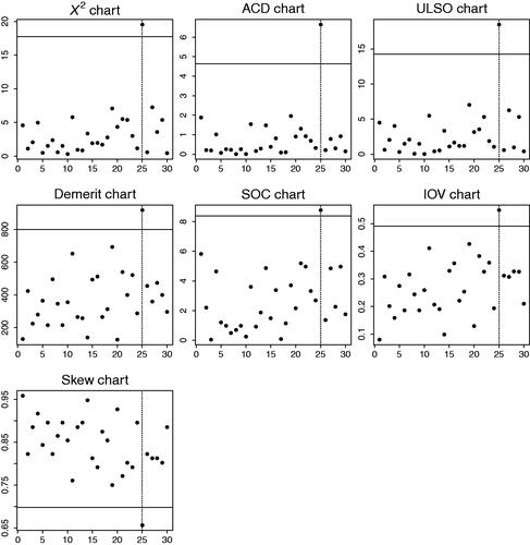
Figure D.2. Memory-type control charts (EWMA version of charts from Figure D.1, or CUSUM and SR) for flash data, where alarm times highlighted by dashed line.

References

- Agresti, A. 2010. Analysis of Ordinal Categorical Data. 2nd edition. Hoboken, New Jersey: John Wiley & Sons, Inc.
- Bai, K., and J. Li. 2021. Location-scale monitoring of ordinal categorical processes. Naval Research Logistics (NRL) 68 (7):937–50. doi: 10.1002/nav.21973.
- Bashkansky, E., and T. Gadrich. 2011. Statistical quality control for ternary ordinal quality data. Applied Stochastic Models in Business and Industry 27 (6):586–99. doi: 10.1002/asmb.868.
- Bross, I. D. J. 1958. How to use ridit analysis. Biometrics 14 (1):18–38. doi: 10.2307/2527727.
- Dodge, H. F. 1928. A method of rating manufactured product. Bell System Technical Journal 7 (2):350–68. doi: 10.1002/j.1538-7305.1928.tb01229.x.
- Dodge, H.F., Torrey, M.N. 1956. A check inspection and demerit rating plan. Journal of Quality Technology 9(3), 146–153.
- Duncan, A. J. 1950. A chi-square chart for controlling a set of percentages. Industrial Quality Control 7:11–5.
- Duran, R. I., and S. L. Albin. 2009. Monitoring and accurately interpreting service processes with transactions that are classified in multiple categories. IIE Transactions 42 (2):136–45. doi: 10.1080/07408170903074908.
- Edwards, H. P., K. Govindaraju, and C. D. Lai. 2007. A control chart procedure for monitoring university student grading. International Journal of Services Technology and Management 8 (4/5):344–54. doi: 10.1504/IJSTM.2007.013924.
- Franceschini, F., and D. Romano. 1999. Control chart for linguistic variables: A method based on the use of linguistic quantifiers. International Journal of Production Research 37 (16):3791–801. doi: 10.1080/002075499190059.
- Franceschini, F., M. Galetto, and M. Varetto. 2005. Ordered samples control charts for ordinal variables. Quality and Reliability Engineering International 21 (2):177–95. doi: 10.1002/qre.614.
- Hakimi, A., H. Farughi, A. Amiri, and J. Arkat. 2021. Phase II monitoring of the ordinal multivariate categorical processes. Advances in Industrial Engineering 55 (3):249–67.
- Jones, L. A., W. H. Woodall, and M. D. Conerly. 1999. Exact properties of demerit control charts. Journal of Quality Technology 31 (2):207–16. doi: 10.1080/00224065.1999.11979915.
- Karlin, S., and H. M. Taylor. 1975. A First Course in Stochastic Processes. 2nd edition. New York: Academic Press.
- Kiesl, H. 2003. Ordinale Streuungsmaße—Theoretische Fundierung und statistische Anwendungen (in German). Lohmar, Cologne: Josef Eul Verlag.
- Klein, I., and M. Doll. 2021. Tests on asymmetry for ordered categorical variables. Journal of Applied Statistics 48 (7):1180–98. doi: 10.1080/02664763.2020.1757045.
- Knoth, S. 2006. The art of evaluating monitoring schemes—How to measure the performance of control charts?. In Frontiers in Statistical Quality Control 8, eds. H.-J. Lenz & P.-T. Wilrich, 74–99. Heidelberg: Physica-Verlag.
- Kvålseth, T. O. 2011a. The lambda distribution and its applications to categorical summary measures. Advances and Applications in Statistics 24 (2):83–106.
- Kvålseth, T. O. 2011b. Variation for categorical variables. In International Encyclopedia of Statistical Science, ed. M. Lovric, 1642–5. Berlin: Springer.
- Lehmann, E. L. 1953. The power of rank tests. The Annals of Mathematical Statistics 24 (1):23–43. doi: 10.1214/aoms/1177729080.
- Li, M., and Q. Lu. 2022. Changepoint detection in autocorrelated ordinal categorical time series. Environmetrics 33 (7):e2752. doi: 10.1002/env.2752.
- Li, J., F. Tsung, and C. Zou. 2014. A simple categorical chart for detecting location shifts with ordinal information. International Journal of Production Research 52 (2):550–62. doi: 10.1080/00207543.2013.838329.
- Li, J., J. Xu, and Q. Zhou. 2018. Monitoring serially dependent categorical processes with ordinal information. IISE Transactions 50 (7):596–605. doi: 10.1080/24725854.2018.1429695.
- Marcucci, M. 1985. Monitoring multinomial processes. Journal of Quality Technology 17 (2):86–91. doi: 10.1080/00224065.1985.11978941.
- Montgomery, D. C. 2009. Introduction to Statistical Quality Control. 6th edition. New York: John Wiley & Sons, Inc.
- Nembhard, D. A., and H. B. Nembhard. 2000. A demerits control chart for autocorrelated data. Quality Engineering 13 (2):179–90. doi: 10.1080/08982110108918640.
- Ottenstreuer, S. 2022. The Shiryaev–Roberts control chart for Markovian count time series. Quality and Reliability Engineering International 38 (3):1207–25. doi: 10.1002/qre.2945.
- Page, E. 1954. Continuous inspection schemes. Biometrika 41 (1-2):100–15. doi: 10.1093/biomet/41.1-2.100.
- Perry, M. B. 2020. An EWMA control chart for categorical processes with applications to social network monitoring. Journal of Quality Technology 52 (2):182–97. doi: 10.1080/00224065.2019.1571343.
- Roberts, S. W. 1959. Control chart tests based on geometric moving averages. Technometrics 1 (3):239–50. doi: 10.1080/00401706.1959.10489860.
- Roberts, S. W. 1966. A comparison of some control chart procedures. Technometrics 8 (3):411–30. doi: 10.1080/00401706.1966.10490374.
- Ryan, A. G., L. J. Wells, and W. H. Woodall. 2011. Methods for monitoring multiple proportions when inspecting continuously. Journal of Quality Technology 43 (3):237–48. doi: 10.1080/00224065.2011.11917860.
- Samimi, Y., A. Aghaie, and M. J. Tarokh. 2010. Analysis of ordered categorical data to develop control charts for monitoring customer loyalty. Applied Stochastic Models in Business and Industry 26 (6):668–88. doi: 10.1002/asmb.808.
- Shewhart, W. A. 1931. Economic Control of Quality of Manufactured Product. New York: D. Van Nostrand Company, Inc.
- Shiryaev, A. N. 1961. The problem of the most rapid detection of a disturbance in a stationary process. Soviet Mathematics: Doklady 2:795–9.
- Steiner, S. H., P. L. Geyer, and G. O. Wesolowsky. 1994. Control charts based on grouped observations. International Journal of Production Research 32 (1):75–91. doi: 10.1080/00207549408956917.
- Steiner, S. H., P. L. Geyer, and G. O. Wesolowsky. 1996a. Shewhart control charts to detect mean and standard deviation shifts based on grouped data. Quality and Reliability Engineering International 12 (5):345–53. doi: 10.1002/(SICI)1099-1638(199609)12:5<345::AID-QRE11>3.0.CO;2-M.
- Steiner, S. H., P. L. Geyer, and G. O. Wesolowsky. 1996b. Grouped data-sequential probability ratio tests and cumulative sum control charts. Technometrics 38 (3):230–7. doi: 10.1080/00401706.1996.10484502.
- Tucker, G. R., W. H. Woodall, and K.-L. Tsui. 2002. A control chart method for ordinal data. American Journal of Mathematical and Management Sciences 22 (1-2):31–48. doi: 10.1080/01966324.2002.10737574.
- Wang, J., J. Li, and Q. Su. 2017. Multivariate ordinal categorical process control based on log-linear modeling. Journal of Quality Technology 49 (2):108–22. doi: 10.1080/00224065.2017.11917983.
- Wang, J., Q. Su, and M. Xie. 2018. A univariate procedure for monitoring location and dispersion with ordered categorical data. Communications in Statistics - Simulation and Computation 47 (1):115–28. doi: 10.1080/03610918.2017.1280159.
- Wardell, D. G., and M. R. Candia. 1996. Statistical process monitoring of customer satisfaction survey data. Quality Management Journal 3 (4):36–50. doi: 10.1080/10686967.1996.11918757.
- Weiß, C. H. 2020. Distance-based analysis of ordinal data and ordinal time series. Journal of the American Statistical Association 115 (531):1189–200. doi: 10.1080/01621459.2019.1604370.
- Weiß, C. H. 2021a. On approaches for monitoring categorical event series. In Control Charts and Machine Learning for Anomaly Detection in Manufacturing, Springer Series in Reliability Engineering, ed. K.P. Tran, 105–29. Cham: Springer Nature Switzerland AG.
- Weiß, C. H. 2021b. Analyzing categorical time series in the presence of missing observations. Statistics in Medicine 40 (21):4675–90. doi: 10.1002/sim.9089.