Abstract
Nanometer distance measurements based on electron paramagnetic resonance methods in combination with site-directed spin labelling are powerful tools for the structural analysis of macromolecules. The software package mtsslSuite provides scientists with a set of tools for the translation of experimental distance distributions into structural information. The package is based on the previously published mtsslWizard software for in silico spin labelling. The mtsslSuite includes a new version of MtsslWizard that has improved performance and now includes additional types of spin labels. Moreover, it contains applications for the trilateration of paramagnetic centres in biomolecules and for rigid-body docking of subdomains of macromolecular complexes. The mtsslSuite is tested on a number of challenging test cases and its strengths and weaknesses are evaluated.
Introduction
Electron paramagnetic resonance (EPR) based distance measurements in biological macromolecules are a valuable complement to crystallography or NMR studies [Citation1–3]. The most commonly used EPR technique for distance measurements is pulsed electron–electron double resonance (PELDOR, also known as DEER) [Citation4]. It can be used to accurately determine interspin distances in the range within 15–80 Å [Citation5]. Since most biological macromolecules are not paramagnetic, site-directed spin labelling (SDSL) with nitroxides is often used to incorporate spins into proteins [Citation6,7] or nucleic acids [Citation8,9]. However, the translation of PELDOR-derived distances into structures is often affected by the flexibility and dimension of the spin labels used. Thus, an accurate model of the conformational distribution of the spin labels attached to the biomolecule is required to draw structural conclusions from the distance data. Since crystallographic studies of multiple spin-labelled mutants of a biomolecule are in general not feasible; this model will in most cases be based on computer simulations. The currently available simulation programs MMM, mtsslWizard and PRONOX that generate such label distributions predict experimental PELDOR distances between two nitroxide spin labels with errors in the range of ∼3 Å [Citation10–12].
Once, a model of the macromolecule has been spin labelled in silico, PELDOR-derived distances can be used to localise individual spin centres such as paramagnetic metal ions or EPR-active substrates of enzymes relative to the model of the macromolecular structure [Citation13,14]. Although the location of metal ions can in most cases be inferred from sequence alignments or crystal structures, in some cases this problem is far from trivial, even if high-resolution structures are available. An example of this is metallonucleases where multiple metal centres can be part of the active site and even movements of the metals during the reaction cycle are proposed [Citation15]. Although crystal structures of these enzymes are available, the location and function of the metal ions are still under debate [Citation15]. Similarly, the localisation of the active site of a novel enzyme (especially non-metallo enzymes) can be difficult, for example, when only a structure of the apo-enyzme is available. The trilateration of spin-labelled or intrinsically EPR-active substrates can in such cases provide a quick and cost-effective solution to locate the active site or a metal-binding site. The general idea of trilateration is the localisation of a certain object in three-dimensional (3D) space by measuring distances between this object and known reference objects [Citation16]. In the context of EPR spectroscopy, spin labels introduced by SDSL would serve as reference objects for the trilateration and the object to be localised would be the intrinsic spin centre, such as a metal ion [Citation14], the spin-labelled or intrinsically EPR-active substrate [Citation13] or additional spin labels [Citation17,18]. Another important application for PELDOR-derived distances is the in silico reconstruction of macromolecular complexes from individual domains. Often, structural information is only available for subunits of such complexes and PELDOR can be used to reconstruct the complex based on distance-constrained rigid-body docking or refinement [Citation19–22]. Results of such experiments can give important insights into the geometry of macromolecular complexes, and thus, serve as a basis for further experiments and structural analysis.
We present here the software package mtsslSuite, which consists of three programs – mtsslWizard, mtsslTrilaterate and mtsslDock. These programs are designed to construct spin-labelled models of macromolecules (mtsslWizard) as well as to use these models for the localisation of spin centres by trilateration (mtsslTrilaterate) or the reconstruction of macromolecular complexes by distance-constrained rigid-body docking (mtsslDock). All three programs can provide scientists with valuable feedback to decide if the available distance constraints support or disagree with a current working model, and if, for example, more labels have to be introduced to get an accurate answer to the problem at hand.
Results and discussion
All programs of the mtsslSuite are designed to work in conjunction with the freely available PyMOL molecular graphics program (www.pymol.org). MtsslTrilaterate and mtsslDock can use the models of spin-labelled macromolecules generated by means of mtsslWizard or other packages as input data. In the following, the usage and the special features of each program will be discussed with the help of examples.
mtsslWizard
The mtsslWizard program allows the user to spin label macromolecules in silico. Its graphical user interface (GUI) is fully integrated into PyMOL. Generally, the user can choose the type of spin label from the mtsslWizard menu (supplementary Figure 1) and then attach the chosen label to the selected residue of a biomolecule by clicking on the amino acid/nucleotide it should be positioned at [Citation10]. The program rotates the spin label around its rotatable bonds in order to explore the volume, which is accessible to the label (‘tether-in-a-cone-model’, [Citation23–27]). MtsslWizard does not consider preferred rotamers of the spin label but only excludes conformations that produce clashes with the macromolecular surface or with a label itself, considering a user-defined cut-off value. The advantages and limitations of this approach are thoroughly discussed in a previous publication [Citation10]. In the following, only the changes between versions (1.0) and (1.1) are discussed.
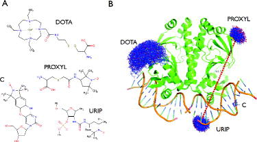
In the first version of MtsslWizard (1.0), only the spin-label MTSSL was included into the program and it was shown that experimental data from a large test data-set (52 distances) can be predicted with an average accuracy of 3 Å, which is on par with other available software packages (MMM, PRONOX). Here, we present an improved version of mtsslWizard (1.1), which contains several new features in comparison with the original version (1.0). Firstly, the algorithm has been optimised, so that the calculation speed has increased and is no longer dependent on the size of the macromolecular model. Secondly, the GUI has been slightly modified in order to make it more comprehensible (supplementary Figure 1). For example, the ‘allowed clashes’ criterion has been merged with the ‘vdW-cut-off’ criterion. The resulting ‘vdW-restraint’ setting can now be switched between two values: ‘tight’ (3.4 Å cut-off, 0 clashes) and ‘loose’ (2.5 Å cut-off, 5 clashes). The ‘loose’ setting allows closer contacts between label and protein, accounting for flexibility of the system. This setting is useful if a site can be experimentally labelled but cannot be labelled in silico using the default ‘tight’ setting, because the static molecular model is too crowded. As discussed previously [Citation10], the value of 2.5 Å was chosen as a minimum cut-off value because it represents the distance between the donor and acceptor of a short hydrogen bond, whereas the 3.4 Å cut-off represents a short vdW interaction (ignoring the hydrogens). The mtsslWizard asks the user to switch to the ‘loose’ setting if less than 10 conformations of a label can be found during a run. Importantly, the new release of mtsslWizard includes several additional spin labels that were requested by users (Figure (A)): the PROXYL spin label, the gadolinium-based DOTA spin label [Citation28] and two spin labels for nucleic acids, the C-label [Citation29] and a urea-based TEMPO spin label (URIP) [Citation30]. Figure (B) shows examples for use of the newly included spin labels. Since mtsslWizard is based on the accessible volume approach, any spin or FRET label with known structure can be easily added as a plug-in to the program, even if no rotamer libraries are available.
Figure 1. New features implemented in mtsslWizard. (A) Structures of the four newly included spin labels. (B) Examples for the use of the spin labels listed in (A). The dashed red line between the PROXYL and URIP labels represents the average distance between these two ensembles. The old version of the program showed all possible distances as lines, which resulted in screen cluttering.
Version (1.1) of the program was benchmarked against the original test data-set [Citation10] consisting of 52 MTSSL-derived distances (Figure (A)). The results confirm that the program can predict experimental data with an accuracy of 3 Å, similar to MMM or PRONOX (see also [Citation31]). The slight deviations in the prediction of some of the interspin distances between this version of mtsslWizard and the original version are due to the simplified clash criterion (see above). For the newly added spin labels, no large experimental data-sets are available, and we therefore cannot provide a similarly extensive benchmark as for the MTSSL spin label. For the PROXYL label, we used mtsslWizard to predict experimental distance distributions from PROXYL-labelled light-harvesting complex II [Citation12]. The overlay of the experimental distance distributions with the ones from mtsslWizard (Figure (B)) shows that the program can predict the PROXYL-based distributions with good accuracy. The DOTA label was tested using a doubly DOTA-labelled transmembrane peptide resulting in good fits of experimental distance distributions [Citation32]. To test the C spin label, a model of a DNA duplex (make-NA server, http://structure.usc.edu/make-na/server.html) was constructed using the sequence of dsDNA1 (fwd: 5′-GATGCGFGCGCGCGACTGAC-3′, rev: 3′-CTACGCGCGCGCGCTGAFTG-5′) from [Citation33] and the C spin label was attached to the positions marked by ‘F’ in the sequence using mtsslWizard. The distance between the modelled C labels is 37.6 Å, close to the experimental value of 36.5 Å Figure (D). Note that due to the rigidity of the C label, it is only attached to the selected nucleotide by mtsslWizard and not rotated in any way. As a test for the URIP label, a double-stranded polyA:T 15mer was experimentally spin labelled using URIP at positions 3 and 8 of the T strand and PELDOR data were recorded (Figure (C)). A model of the labelled DNA strand was constructed using the make-NA server (http://structure.usc.edu/make-na/server.html), PyMOL and mtsslWizard. Figure (C) shows that experimental data (mean distance 27.7 Å [DeerAnalysis) and prediction (mean distance 27.0 Å) fit well.
Figure 2. Benchmarking of mtsslWizard. (A) Comparison of version (1.0) of mtsslWizard (grey boxes) with version (1.1) (white circles). Experimental distances that were included in the benchmark data-set of the original mtssWizard paper are plotted against predictions of versions (1.0) and (1.1) of mtsslWizard. The x-axis shows the experimental distance and the y-axis shows the difference of the experimental value to the prediction. The ideal y = 0 line is marked in red, the areas corresponding to different prediction errors are shaded with different colours (green: <3 Å, yellow: ≤5 Å and white: >5 Å). (B) Comparison of experimental distance distributions of the PROXYL-labelled light harvesting complex II (black line, digitised from [Citation12], PDB-ID: 2BHW) with mtsslWizard predictions (red line). (C) Example for the use of the URIP label. The experimental distance distribution is shown in black and the prediction based on the model shown in the inset is shown in red. (D) Example for the use of the C spin label. The experimental distance distribution (black) was constructed using data from [Citation33]. The red vertical line highlights the distance that was calculated by mtsslWizard. The inset shows the DNA (cartoon model) and the modelled spin label (spheres).
![Figure 2. Benchmarking of mtsslWizard. (A) Comparison of version (1.0) of mtsslWizard (grey boxes) with version (1.1) (white circles). Experimental distances that were included in the benchmark data-set of the original mtssWizard paper are plotted against predictions of versions (1.0) and (1.1) of mtsslWizard. The x-axis shows the experimental distance and the y-axis shows the difference of the experimental value to the prediction. The ideal y = 0 line is marked in red, the areas corresponding to different prediction errors are shaded with different colours (green: <3 Å, yellow: ≤5 Å and white: >5 Å). (B) Comparison of experimental distance distributions of the PROXYL-labelled light harvesting complex II (black line, digitised from [Citation12], PDB-ID: 2BHW) with mtsslWizard predictions (red line). (C) Example for the use of the URIP label. The experimental distance distribution is shown in black and the prediction based on the model shown in the inset is shown in red. (D) Example for the use of the C spin label. The experimental distance distribution (black) was constructed using data from [Citation33]. The red vertical line highlights the distance that was calculated by mtsslWizard. The inset shows the DNA (cartoon model) and the modelled spin label (spheres).](/cms/asset/ebf07016-03be-4078-ab69-055073fa65f2/tmph_a_809804_f0002_oc.jpg)
mtsslTrilaterate
The mtsslTrilaterate program can be used to locate spin centres in the structure of biomolecules by means of trilateration, for example, to find metal- or substrate-binding sites (see above).
Once the trilateration program has been launched via the PyMOL menu, its GUI appears as shown in supplementary Figure 2(A). The trilateration process can be prepared by importing the attached spin labels and experimental distances into the program as explained in the software manual (www.pymolwiki.org). The distance data itself can be entered in two different ways: manually or by import of data files. The program can, for example, import DeerAnalysis [Citation34] interspin distance distributions. The program solves the trilateration problem in two steps. In the first step, the coordinates of the unlocalised spin centre are estimated by means of singular value decomposition (SVD). The result of this step is needed as an ‘initial guess’ for the nonlinear least squares (NLS) optimisation. The goal of NLS algorithms is the minimisation of the commonly used χ2 merit function,
(1) where l is the number of the spin label, (xlylzl) are coordinates of the l spin label, rl and σl are the mean value and the standard deviation of the distance between the l spin label and the unlocalised spin centre. Here, (xyz) are the unknown coordinates of the spin centre. They are incremented in each iteration and the corresponding value of χ2 is calculated. Then, the program checks whether the obtained χ2 is decreased by a factor of less than 10−3 after the last iteration. If this criterium is satisfied, the problem is considered to be solved. The NLS algorithm uses either the inverse-Hessian method or the Levenberg–Marquardt method [Citation35]. The user can choose the algorithm in the ‘Preferences’ menu (supplementary Figure 2(B) and (C)). In our hands, both algorithms produce exactly the same results. For each algorithm, a number of parameters can be set in the ‘Preferences’ menu (supplementary Figure 2(B) and (C)). These settings include the maximum number of iterations, the minimal χ2 value (below which the problem is considered solved) and the damping parameter lambda (used only for the Levenberg–Marquart algorithm). The values used as default were found to be optimal for the test cases described below. Further description of these parameters can be found elsewhere [Citation35]. The solution of the trilateration problem can be interpreted as the most probable coordinates of the unlocalised spin centre and their standard errors. These data are presented as a table in the ‘Output’ panel (supplementary Figure 2(A)) and can optionally be visualised graphically inside PyMOL (Figures and ). The calculation statistics are presented in terms of the obtained χ2 value and the number of NLS iterations used to reach this χ2. The χ2 value shows how precisely the trilateration problem was solved for the given set of input data. A lower value of χ2 corresponds to a lower uncertainty in the coordinates obtained. The factors that affect the χ2 value are the number of spin labels used to localise the intrinsic spin centre, the precision and the dispersion of the distances evaluated from PELDOR time traces and the accuracy of the model of the spin-labelled biomolecule.
Figure 3. Trilateration of the LOPTC lipid in soybean seed lipoxygenase-1 (SBL1). (A) SBLI is shown as green cartoon model. The MTSSL ensembles that were generated with mtsslWizard are shown as blue and red stick models. The trilateration spheres whose radii correspond to the experimental LOPTC-MTSSL distances are shown in cyan. The trilateration result (‘target’) is represented as an orange ellipsoid and marks the position of the LOPTC lipid. (B) Close up of the ‘target’ area. The protein is shown as green cartoon model; selected amino acid residues are shown as sticks. The target is represented by a translucent orange ellipsoid. The magenta spheres inside the ellipsoid are the results of 10 independent attempts of docking LOPTC into SBLI with mtsslDock (marked by arrow).
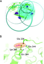
Figure 4. Trilateration of the inhibitory copper-binding site in EcoRI. The EcoRI:DNA complex is shown as a white cartoon model. The MTSSL ensembles that were generated with mtsslWizard are shown as blue and red stick models. The trilateration spheres whose radii correspond to the experimental Cu-MTSSL distances are shown in cyan. All histidine residues in the dimeric structure are highlighted as purple spheres. His114 that was identified as the Cu2+ binding site in [Citation14] is marked and is in the closest proximity to both trilateration spheres. The red spheres (marked by a arrow) represent the result of 10 independent attempts of docking the Cu2+ ion into the complex structure with mtsslDock.
![Figure 4. Trilateration of the inhibitory copper-binding site in EcoRI. The EcoRI:DNA complex is shown as a white cartoon model. The MTSSL ensembles that were generated with mtsslWizard are shown as blue and red stick models. The trilateration spheres whose radii correspond to the experimental Cu-MTSSL distances are shown in cyan. All histidine residues in the dimeric structure are highlighted as purple spheres. His114 that was identified as the Cu2+ binding site in [Citation14] is marked and is in the closest proximity to both trilateration spheres. The red spheres (marked by a arrow) represent the result of 10 independent attempts of docking the Cu2+ ion into the complex structure with mtsslDock.](/cms/asset/abe742da-378b-4710-bcd1-e2f189017ff9/tmph_a_809804_f0004_oc.jpg)
We tested the mtsslTrilaterate program for soybean seed lipoxygenase-1 (SBL1) using a data-set of PELDOR-derived distances published by Gaffney et al. [Citation13]. The data-set consists of five distances measured between the TEMPO-labelled lipid (LOPTC) and five spin labels that were attached to lipoxygenase by SDSL. In the original paper, these data were used to localise the polar end of the LOPTC on the molecular surface of lipoxygenase by means of trilateration using multi-dimensional scaling and Procrustes analysis that are included in the MATLAB (http://www.mathworks.de) statistical toolbox. The mtsslTrilaterate program was run with the input parameters listed in Table . The coordinates of the spin labels were obtained by using mtsslWizard and the crystal structure of SBL1 (PDB:1YGE, [Citation36]). The mean values and standard deviations of the interspin distances between LOPTC and five spin labels were taken from [Citation13]. Calculations were performed with the default settings of mtsslTrilaterate (see supplementary Figure 2(B) and (C)). The results are shown in Figure and Table . As can be seen from Figure , the program places the LOPTC spin centre next to helices 2 and 11 of SBL1. In this position, LOPTC is surrounded by amino acids Glu236, Lys260, Gln264 and Gln544 (Figure (B)). Within the error of calculations, the trilateration result coincides with those published in the original paper (Table ). A slight deviation between these two solutions may be related to the usage of different models of the spin-labelled protein (either derived from mtsslWizard or PRONOX) and different calculation procedures. To estimate the influence of differences in the models on the solution, the mtsslTrilaterate program was run with the coordinates of the spin labels taken from [Citation13]. It was found that the coordinates of the LOPTC spin derived in this way fit with high precision to the published coordinates. This fact indicates that the small deviations between the solutions are related to the differences in the models of spin-labelled protein. With mtsslTrilaterate, this localisation of LOPTC was done within 10 min, including the in silico spin labelling of the labelled positions with mtsslWizard.
Table 1. Calculated coordinates of spin centres in the molecular coordinate system of soybean seed lipoxygenase-1 (PDB:1YGE) and PELDOR-derived distances between these centres and LOPTC.
As a second test case, we took an experimental data-set that was used to localise an inhibitory copper-binding site in the restriction endonuclease EcoRI [Citation14]. Position Ser180 in both monomers of the dimeric protein (PDB-ID: 1CKQ) was labelled with mtsslWizard and the experimental distances between the spin label and the copper site to be localised were used as input for mtsslTrilaterate. Although these input data are not sufficient for the program to solve the trilateration with a unique solution (at least four distances are needed for this), the visualisation of the trilateration spheres in PyMOL (Figure ) shows that the point of closest approach of the two spheres coincides with His114, which was also identified as the Cu2+ binding site in the original paper.
mtsslDock
The mtsslDock program enables the user to dock two macromolecules based on a set of experimental PELDOR distances. The program requires models of the spin-labelled macromolecules and the experimental distance data between them as input. The structural models can be spin labelled with mtsslWizard or other available software packages.
After launching mtsslDock from within PyMOL, its GUI appears as shown in supplementary Figure 3. The docking process is then prepared by importing the spin-labelled docking partners into the program as explained in the software manual (www.pymolwiki.org). In the following, the algorithm and the adjustable settings are explained: mtssldock uses a mixed genetic and evolutionary algorithm [Citation37] to find docking models between two macromolecules (e.g. proteins A and B) that agree to the experimental distance data. The principle of genetic and evolutionary algorithms is based on natural evolution where inheritance, mutation and genetic crossover between generations lead to a population with increased fitness for survival in the particular environment. Such algorithms have been used for a wide array of problems, including protein–protein docking based on surface complementarity [Citation38] or molecular replacement in crystallographic phasing [Citation39]. The algorithm works as follows: protein A is held fixed in space, while in the first step of the calculation, mtsslDock generates a population of 400 random orientations (each orientation is called a chromosome) of protein B. A chromosome is a set of six numbers (‘genes’), which determine the translation and rotation of the protein in 3D space: x, y, z, α, β, γ (see also supplementary Figure 4). The root-mean-square difference (RMSD) between the experimental distances and distances derived from the current docking model as well as the χ2 value (as specified in EquationEquation (1)(1) , see above) are then determined. The χ2 value is used as a surrogate for the fitness of the particular chromosome – here, a low χ2 value corresponds to a higher fitness than a high χ2 value. In the next step, the 5% least-fit chromosomes of the population are discarded and replaced by ‘offspring’ of the surviving chromosomes (supplementary Figure 4). The offspring is generated by genetic operations: random mutagenesis, small creep mutagenesis, exchange crossover or single-point crossover (e.g. [Citation38], supplementary Figure 4), forming a new generation of the population. This process is repeated 1000 times before a ‘packing-function’ adds a high fitness penalty to chromosomes that lead to protein B clashing into protein A (only Cα atoms are considered; a distance lower than 3.4 Å between two Cα atoms is counted as a clash). The 5% fittest trial orientations are then used as starting orientations for a second evolution with 50 generations in which only small creep mutations (supplementary Figure 4) are introduced to the fittest chromosome to replace the 95% unfittest chromosomes in each step. Here, the fitness is determined by scoring χ2 as well as clashes between both proteins. This effectively resembles a least-squares rigid-body refinement. In some cases, conformational changes of the docking partners between the bound- and unbound state might lead to ‘false negative’ docking results due to the clash criterion. To account for this, mtsslDock does not simply discard clashing solutions but displays them marked as ‘clashing’ inside the GUI and within PyMOL, so that ultimately the user decides whether a solution should be discarded or not.
By default, the program calculates 10 independent populations and exports the fittest solution of each population to PyMOL to be investigated by the user. A docking calculation takes between 0.5 and 5 min for a single population on a standard laptop, depending on the settings that were used and the size of the molecules (due to the clash scoring). We recommended to do the calculation with at least 10 independent populations to get an impression of how statistically significant the produced solutions are.
The robustness of the algorithm was analysed using the crystal structure of the protein–protein complex rubredoxin:rubredoxin-reductase (PDB-ID: 2v3b, [Citation40]). The rubredoxin reductase was kept static (protein A), while rubredoxin was allowed to be moved by mtsslDock (protein B). Both proteins were spin labelled at 12 positions with mtsslWizard (supplementary Figure 5), and 4–12 of the 144 possible distances were randomly selected as constraints. Each label was only allowed to contribute to one distance constraint. Because of the statistic nature of the docking algorithm, the results of this analysis have to be regarded in terms of the ability of the algorithm to reliably find a correct docking solution with a given number of constraints. For the purpose of our benchmark, we arbitrarily define a correct solution as one that has an RMSD (all atoms) to the experimental position of protein B of less than 2.5 Å. Figure (A) (top) shows that in each docking run of our benchmark, the algorithm found potential solutions that fit to the ‘experimental’ distances with RMSD values <1 Å. However, only when six or more constraints were used, was the correct solution among the docked structures (Figure (A), bottom). With an increasing number of constraints, the fraction of wrong solutions decreased, simply because it becomes less likely for the algorithm to find an additional solution that satisfies all distance constraints (Figure (A), bottom). Figure (B) and (C) shows the docking solutions when 7 or 10 constraints were used, respectively. Whereas all solutions were correct when 10 constraints were used (Figure (C)), the 10 solutions derived from the 7 constraints form 2 clusters (Figure (B), red and green), one of which is located at the correct position. For both the clusters, all solutions show a similar fit to the ‘experimental data’ with RMSD <1 Å (Figure (A), top). Importantly, this is much lower than the uncertainty that is on average introduced by in silico spin labelling (∼3 Å) [Citation10,Citation31] and experimental errors. Figure (D) shows that interestingly, the ‘worst’ solution of the correct cluster has a χ2 value that is higher than that of the incorrect solutions. Thus, in reality, right and wrong solutions cannot simply be distinguished by ranking the solutions. In our benchmark case, it would be straightforward to identify the correct cluster of protein B, since the wrong solutions do not make any contact with protein A. However, in reality and especially in cases, where, for example, a domain of the protein complex is missing from the structure, more constraints would have to be added to get a definite answer.
Figure 5. Analysis of the mtsslDock algorithm. (A) Benchmark results. Top: Each black or blue dot represents the result of an independent docking run that was performed with the number of constraints indicated on the x-axis. The y-axis (logarithmic scale) represents the RMSD between the ‘experimental’ distances and the distances retrieved from the docking result. The black dots represent the docking runs performed with rubredoxin:rubredoxin-reductase, and the blue dots, the docking runs performed with Cap (see main text). Bottom: The graph is analogue to the top panel but shows the RMSD difference between the docking result and the experimentally found position of the docked molecule. The area with green shading represents RMSD values <2.5 Å, yellow: ≤5 Å, red: >5 Å. (B) Docking results (red, green) for rubredoxin:rubredoxin-reductase (magenta:orange) with seven constraints. (C) Same as B, but 10 constraints were used. (D) Fitness traces of the docking runs for the solutions shown in (B). The traces are coloured according to the solutions in (B).
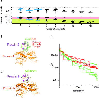
Proteins often form functional dimers and sometimes only the monomeric structure or competing dimer models can be derived from crystallography. PELDOR can in such cases be used to determine the native dimer structure [Citation22]. We thus added an option to mtsslDock that only C2 symmetric docking models are constructed and evaluated during the docking run. In theory, less constraints (and therefore experimental time) should be needed in such cases, because the system has less degrees of freedom. We analysed this function of mtsslDock with the same benchmark, but used the structure of the dimeric Cap protein (Figure (A), PDB-ID: 1O3Q) as a test case. This time, six labels were attached to each monomer (at corresponding positions) of the protein (supplementary Figure 5) and six, five or four distances between monomers were randomly chosen as constraints. Figure (A) (blue dots) shows, that as expected, correct solutions can be found with down to four constraints. More symmetry restraints will be added in future releases of the software.
In summary, our algorithm can reliably dock two structures when enough distance constraints are available (six or more for unsymmetric structures, four or more for C2 symmetric structures). It cannot distinguish a correct from an incorrect solution when distances derived from both solutions show a similarly good fit to the experimental distances. This situation can arise when not enough constraints are present, when the algorithm gets trapped in local minima or from specific placements of labels. For example, when three labels were placed on protein A, they would form a mirror plane for any number of labels on protein B, and the algorithm would not be able to distinguish the solution from its mirror image.
We also tested mtsslDock with three published sets of experimental interspin distances. The first example is the complex between the cytoplasmic domain of erythrocyte band 3 and ankyrin-R repeats 13–24 [Citation20]. This complex has been investigated by various biochemical and biophysical techniques, including a set of 20 PELDOR measurements. In the original paper, the PELDOR-derived distances were used as distance constraints for docking analysis with RosettaDock [Citation41], resulting in a model of the protein complex that is in agreement with other biochemical and biophysical data [Citation20]. To dock the complex with mtsslDock, we labelled the experimentally used sites in both proteins with mtsslWizard, imported the mean coordinates of the labels into mtsslDock and entered the 20 experimental distances and standard deviations [Citation20]. The result of the docking calculation (10 docking runs were used, calculation time: 30 min) is shown in Figure and resembles the result that was obtained in the original publication (supplementary Figure 5). Interestingly, the program produces two clusters of possible solutions, which have similar fitness scores (Figure , supplementary Figure 5). Both of these clusters are contained in the ensemble of the published solutions. Since the number of constraints in this case greatly exceeds six (see above and Figure (A)), it seems surprising that our algorithm does not find a single solution. There are several possible reasons for this: (1) some of the distances might be incompatible with each other due to in silico spin-labelling uncertainties and/or experimental uncertainties, (2) the algorithm might get trapped in local minima or (3) some of the constraints are not linearly independent from each other. The latter reason could arise from the fact that in this case most labels were (understandably) repeatedly used for distance measurements. More linearly independent constraints would have to be introduced to resolve this ambiguity. In the original publication, the authors did this by introducing constraints from orthogonal methods, such as solvent accessibility and cross-linking data.
Figure 6. Docking of the cytoplasmic domain of erythrocyte band 3, and ankyrin-R repeats 13–24 [Citation20]. The docking solutions for the ankyrin structure based on 20 PELDOR distances are shown as orange loop models. The erythrocyte band 3 dimer is shown as cartoon model (green and blue). MtsslDock finds two solutions for the problem (solution I and solution II). In the bottom panel, the structure is rotated by 90°.
![Figure 6. Docking of the cytoplasmic domain of erythrocyte band 3, and ankyrin-R repeats 13–24 [Citation20]. The docking solutions for the ankyrin structure based on 20 PELDOR distances are shown as orange loop models. The erythrocyte band 3 dimer is shown as cartoon model (green and blue). MtsslDock finds two solutions for the problem (solution I and solution II). In the bottom panel, the structure is rotated by 90°.](/cms/asset/59693ad4-271b-4416-a27b-29848c2a6b49/tmph_a_809804_f0006_oc.jpg)
The mtsslDock approach can also be used to solve the trilateration problem (see above). For this purpose, we used the SBL-1 example (see mtsslTrilaterate above) and imported the mean coordinates of the five spin labels, the coordinates of an atom that was used as a surrogate for the position of the LOPTC lipid (termed ‘pseudoatom’ below) and the five experimental interspin distances into mtsslDock. The docking was performed using the default settings. Figure (B) (purple spheres) shows that the program places the pseudoatom into the centre of the ‘target’ ellipsoid that was generated by mtsslTrilaterate. Similarly mtsslDock was also used to compute the position of the copper-binding site in EcoRI (see above, [Citation14]). The result of this calculation lies exactly between the two trilateration spheres that were output by mtsslTrilaterate and close to His114, which was identified as the copper-binding site in the original publication (Figure , red spheres). Note that the program would output a range of differing solutions spread on an intersection circle if the two triangulation spheres would intersect each other. Thus, this result has to be considered as a special case. These two examples represent a cross-check of both algorithms. The use of mtsslTrilaterate is, however, recommended in such cases since it is faster, calculates statistics and provides more informative output for the trilateration problem.
Conclusion
The mtsslSuite currently contains a set of three applications that allow in silico spin labelling of macromolecules, localising spin centres with respect to reference spin centres or docking macromolecules based on experimental spin-pair distance constraints.
The programs can import spin-labelled locations that were generated with mtsslWizard but do at the same time offer users the opportunity to use input data from other sources (e.g. MMM or PRONOX). We have shown that all the three programs achieve results that are comparable in precision to those obtained by means of other computational strategies. The source code of all the three programs is freely available at (www.pymolwiki.org).
Supplementary material
Download Zip (443.5 KB)Supplementary material
Download MS Word (642.8 KB)Acknowledgements
We would like to thank Jason Vertrees and Thomas Holder for help concerning PyMOL programming and Damien Farrell for help with the tkinterTable class for mtsslDock. This work has been supported by the SFB813 projects C8 and A6 of the Deutsche Forschungsgemeinschaft (DFG) and the Wellcome Trust (091825/Z/10/Z).
Note added in proof
While this paper went into production, the K1 spin label [42] was added to mtsslWizard upon user request. Supplementary Figure 7 shows a comparison between predicted and experimental distance distributions derived from this spin label.
References
- G. Jeschke, Annu. Rev. Phys. Chem. 63, 419 (2012).
- G.W. Reginsson and O. Schiemann, Biochem. J. 434, 353 (2011).
- O. Schiemann and T.F. Prisner, Q. Rev. Biophys. 40, 1 (2007).
- A. Milov, K. Salikohov, and M. Shirov, Fizika. Tverdogo. Tela. 23, 975 (1981).
- G. Jeschke, A. Bender, and H. Paulsen, J. Magn. Reson. 169, 1–12 (2004).
- C. Altenbach, T. Marti, H.G. Khorana, and W.L. Hubbell, Science 248, 1088 (1990).
- J.P. Klare and H.-J. Steinhoff, Photosyn. Res. 102, 377 (2009).
- S.A. Shelke and S.T. Sigurdsson, Eur. J. Org. Chem. 2012, 2291 (2012).
- R. Ward and O. Schiemann, Structural Information from Oligonucleotides (Springer, Berlin, 2012).
- G. Hagelueken, R. Ward, J.H. Naismith, and O. Schiemann, Appl. Magn. Reson. 42, 377 (2012).
- M.M. Hatmal, Y. Li, B.G. Hegde, P.B. Hegde, C.C. Jao, R. Langen, and I.S. Haworth, Biopolymers 97, 35 (2011).
- Y. Polyhach, E. Bordignon, and G. Jeschke, Phys. Chem. Chem. Phys. 13, 2356 (2011).
- B.J. Gaffney, M.D. Bradshaw, S.D. Frausto, F. Wu, J.H. Freed, and P. Borbat, Biophys. J. 103, 2134 (2012).
- Z. Yang, M.R. Kurpiewski, M. Ji, J.E. Townsend, P. Mehta, L. Jen-Jacobson, and S. Saxena, Proc. Nat. Acad. Sci. U.S.A. 109, E993–1000 (2012).
- C.M. Dupureur, Curr. Opin. Chem. Biol. 12, 250 (2008).
- A. Muschielok, J. Andrecka, A. Jawhari, F. Brückner, P. Cramer, and J. Michaelis, Nat. Methods 5, 965 (2008).
- P.P. Borbat, H.S. Mchaourab, and J.H. Freed, J. Am. Chem. Soc. 124, 5304 (2002).
- G. Jeschke, A. Bender, T. Schweikardt, G. Panek, H. Decker, and H. Paulsen, J. Biol. Chem. 280, 18623–18630 (2005).
- D. Hilger, Y. Polyhach, E. Padan, H. Jung, and G. Jeschke, Biophys. J. 93, 3675 (2007).
- S. Kim, S. Brandon, Z. Zhou, C.E. Cobb, S.J. Edwards, C.W. Moth, C.S. Parry, J.A. Smith, T.P. Lybrand, E.J. Hustedt, and A.H. Beth, J. Biol. Chem. 286, 20746 (2011).
- R. Ward, M. Zoltner, L. Beer, H. El-Mkami, I.R. Henderson, T. Palmer, and D.G. Norman, Structure 17, 1187 (2009).
- M. Zoltner, D.G. Norman, P.K. Fyfe, H. El-Mkami, T. Palmer, and W.N. Hunter, Structure 21, 595–603 (2013).
- N. Alexander, M. Bortolus, A. Al-Mestarihi, H. Mchaourab, and J. Meiler, Structure 16, 181 (2008).
- Z. Guo, D. Cascio, K. Hideg, and W. Hubbell, Protein Sci. 17, 228 (2008).
- S.J. Hirst, N. Alexander, H.S. Mchaourab, and J. Meiler, J. Struct. Biol. 173, 506 (2011).
- E. Hustedt, R. Stein, L. Sethaphong, S. Brandon, Z. Zhou, and S. DeSensi, Biophys. J. 90, 340 (2006).
- Z. Zhou, S.C. DeSensi, R.A. Stein, S. Brandon, M. Dixit, E.J. McArdle, E.M. Warren, H.K. Kroh, L. Song, C.E. Cobb, E.J. Hustedt, and A.H. Beth, Biochemistry. 44, 15115 (2005).
- Y. Song, T.J. Meade, A.V. Astashkin, and E.L. Klein, J. Magn. Reson. 210, 59 (2011).
- P. Cekan, A.L. Smith, N. Barhate, B.H. Robinson, and S.T. Sigurdsson, Nucleic Acids Res. 36, 5946 (2008).
- T.E. Edwards, T.M. Okonogi, and B.H. Robinson, J. Am. Chem. Soc. 123, 1527 (2001).
- G. Jeschke, Prog. Nucl. Magn. Reson. Spectrosc. 72, 42–60 (2013).
- D. Goldfarb (private communication).
- O. Schiemann, P. Cekan, D. Margraf, T.F. Prisner, and S.T. Sigurdsson, Angew. Chem. Int. Edit. 48, 3292 (2009).
- G. Jeschke, V. Chechik, P. Ionita, A. Godt, H. Zimmermann, J. Banham, C. Timmel, D. Hilger, and H. Jung, Appl. Magn. Reson. 30, 473 (2006).
- B.P. Flannery, W.H. Press, and S.A. Teukolsky, Numerical Recipes in C. (Cambridge University Press, New York, 1992).
- W. Minor, J. Steczko, O.B. Stec, and Z. Otwinowski, Biochemistry 35, 10687 (1996).
- M. Srinivas and L.M. Patnaik, Computer 27, 17 (1994).
- E.J. Gardiner, P. Willett, and P.J. Artymiuk, Proteins 44, 44 (2001).
- C.R. Kissinger, D.K. Gehlhaar, and D.B. Fogel, Acta Crystallogr. D. Biol. Crystallogr. 55, 484 (1999).
- G. Hagelueken, L. Wiehlmann, T.M. Adams, H. Kolmar, D.W. Heinz, B. Tümmler, and W.-D. Schubert, Proc. Nat. Acad. Sci. U.S.A. 104, 12276 (2007).
- S. Lyskov and J.J. Gray, Nucleic Acids Res. 36, W233 (2008).
- M.R. Fleissner, E.M. Brustad, T. Kálái, C. Altenbach, D. Cascio, F.B. Peters, K. Hideg, S. Peuker, P.G. Schultz, and W.L. Hubbell, Proc. Nat. Acad. Sci. U.S.A. 106, 21637–21642 (2009).