Fluid–fluid coexistence in an athermal colloid–polymer mixture: thermodynamic perturbation theory and continuum molecular-dynamics simulation

Abstract

Using both theory and continuum simulation, we examine a system comprising a mixture of polymer chains formed from 100 hard-sphere (HS) segments and HS colloids with a diameter which is 20 times that of the polymer segments. According to Wertheim's first-order thermodynamic perturbation theory (TPT1) this athermal system is expected to phase separate into a colloid-rich and a polymer-rich phase. Using a previously developed continuous pseudo-HS potential [J. F. Jover, A. J. Haslam, A. Galindo, G. Jackson, and E. A. Muller, J. Chem. Phys. 137, 144505 (2012)], we simulate the system at a phase point indicated by the theory to be well within the two-phase binodal region. Molecular-dynamics simulations are performed from starting configurations corresponding to completely phase-separated and completely pre-mixed colloids and polymers. Clear evidence is seen of the stabilisation of two coexisting fluid phases in both cases. An analysis of the interfacial tension of the phase-separated regions is made; ultra-low tensions are observed in line with previous values determined with square-gradient theory and experiment for colloid–polymer systems. Further simulations are carried out to examine the nature of these coexisting phases, taking as input the densities and compositions calculated using TPT1 (and corresponding to the peaks in the probability distribution of the density profiles obtained in the simulations). The polymer chains are seen to be fully penetrable by other polymers. By contrast, from the point of view of the colloids, the polymers behave (on average) as almost-impenetrable spheres. It is demonstrated that, while the average interaction between the polymer molecules in the polymer-rich phase is (as expected) soft-repulsive in nature, the corresponding interaction in the colloid-rich phase is of an entirely different form, characterised by a region of effective intermolecular attraction.

Keywords:

• hard sphere
• chains
• polymers
• colloids
• mixtures
• depletion interaction
• thermodynamic perturbation theory
• demixing
• potential of mean force

View correction statement:

Corrigendum

1. Introduction

Colloid–polymer mixtures are present in many substances commonly encountered in everyday life, such as foods and paints, as well as being pervasive in biological systems. They have been found to exhibit a variety of scientifically interesting or practical behaviour [1], and their importance is reflected in the large body of work that has been devoted to their study. Experimental investigations of the phase behaviour of colloid–polymer mixtures have been performed on a variety of systems ranging from comparatively simple latex–polystyrene and silica–polydimethylsiloxane colloidal dispersions to biological systems containing proteins or DNA [2–13]. Phase separation has been described by many authors [3, 4,8,14–27]; see the excellent book of Lekkerkerker and Tuinier [1] for a comprehensive historical review. Fluid-solid coexistence is observed when the radius of gyration of the polymer is small compared to that of the colloid; here one can draw an analogy between the behaviour of the colloids and that of a system of pure hard spheres (HSs). On the other hand, by increasing the ratio of the size of the polymers to that of the colloids one can induce a departure from HS-like phase behaviour; when the polymers are sufficiently large, fluid-phase separation between low-density and high-density colloidal phases is observed; at higher densities solid colloidal phases can also be found.

An important concept in understanding the phase behaviour of colloid–polymer mixtures is that of the depletion interaction. Asakura and Oosawa were the first to recognise this idea in two seminal papers [28,29] published over 50 years ago, and the concept was later reprised by Vrij and co-workers [14,30]. Each colloid is imagined to be surrounded by a so-called depletion layer. When two colloids lie in close proximity the depletion layers overlap and the volume available to the polymer chains increases; as a consequence, the free energy of polymer chains is minimised when the colloids are close together. The overall behaviour can be described in terms of an effective attraction between the colloids, which can give rise to aggregation or phase separation into polymer-rich and colloid-rich fluid phases, often referred to as colloidal vapour and colloidal liquid (respectively). Thorough explanations of the depletion interaction are provided in, for example, references [1,31–35]; depletion forces have been the focus of a number of studies, including [36–43]. In particular, Binder et al. [35] have provided a detailed appraisal of the Asakura–Oosawa (AO) model, and its scope. Accordingly, we provide here only a brief summary.

The AO model is defined through the interactions between the species in the colloid–polymer mixture. Both colloid and polymer are modelled as spherical; the colloids are hard, while the polymers are hard with respect to the colloids but are treated simply as soft, interpenetrating spheres with respect to each other. This model, or the related AO approximation, in which the polymers are treated as ideal chains, has formed the basis of much of the subsequent theoretical work on colloid–polymer systems. An important example in the context of our current paper is the work of Gast and co-workers [16,18], who used thermodynamic perturbation theory [44,45] to predict the phase behaviour of an AO model colloid–polymer mixture; they were able to account for the change from fluid–crystal to fluid–fluid coexistence with increasing polymer size, observing the transition at a size ratio q = R _g/R _c $\gtrsim$ 1/3, where R _g is the radius of gyration of the polymer and R _c is the radius of the colloid. Gast et al. [16] discussed at some length the limitations to their approach brought about by the neglect of three- and higher-body interactions. Later Lekkerkerker et al. [46] introduced the free-volume approach for the determination of the phase behaviour, which captures some of the effects of many-body interactions, as well as avoiding the assumption of Gast et al. that the polymer concentration is the same in the coexisting phases thereby incorporating partitioning of the polymer between phases.

To date, the phase behaviour of colloid–polymer mixtures has been addressed in a number of theoretical studies, in addition to those already mentioned; see, for example, references [34,43,47–57]. Among these, we highlight the studies [43,53–55,58] based on Wertheim's first-order thermodynamic perturbation theory (TPT1) [59,60]; these deal with the polymer at the monomer segment level [61], in contrast to studies based on the AO model or the AO approximation. While it is gratifying that theoretical studies can be used to explain the phase separation seen experimentally, to assess the quality of the underlying models one still requires accurate verification of theories by direct molecular simulation.

Simulations of prototypical colloid–polymer systems have been conducted at different levels of sophistication, e.g., using one-component [48,62] and two-component [37,38,63–72] descriptions; see reference [35] for a review of simulation studies in relation to the AO model. In the approach pioneered by the Hansen group in Cambridge [38,73–77], the ‘polymer as soft colloids’ model is adopted; the simulation of sufficiently large systems is facilitated by a coarse-grained approach in which the polymer–polymer interactions are incorporated using an effective potential that acts between the centres of mass of the chains. Vink and Horbach [78] have also introduced ‘cluster moves’ that allow tractable simulation of the AO and related models using grand canonical Monte Carlo [70,79–81]. An alternative approach to simulate large systems has been lattice Monte Carlo, using an explicit (monomer) description of the polymers ([36,82]). However off-lattice simulations of a system with an explicit model are rare. Starr et al. [83] simulated a system consisting of Lennard-Jones (LJ) chain polymers and nanoparticles, represented by LJ spheres bonded together in an icosahedron, however these authors did not observe phase separation; rather, they reported that the nanoparticle clustering was akin to equilibrium polymerisation. Lo Verso et al. [84] have simulated the interesting and related system of polymer-brush-coated spherical nanoparticles, but the nature of their model precludes phase separation of the type that is of interest in our current work. More recently, Meng et al. [72] simulated systems of LJ-chain polymers and nanoparticles conceptualised as multiple LJ centres grouped together to form larger colloidal spheres; the potentials of interaction between the colloidal nanoparticles, and between nanoparticles and polymer LJ segments were obtained via integration of all the LJ sites in the nanoparticles. Although these authors examined the phase transitions in the system, these were of solid–fluid nature (rather than fluid–fluid), except when monomeric LJ particles were used as solvent in place of the polymers. Also of particular relevance to our current study is the series of papers by Panagiotopoulos and co-workers [71,85–87]. Mahynski et al. [85] performed continuum simulations to complement their more extensive study [71] in which the polymer chains were constrained to lie on a lattice. However, in these two contributions the authors were primarily interested in the so-called protein limit, where the polymer radius of gyration exceeds the colloid radius. By contrast, in our current work, we consider a system corresponding to the colloid limit, which is characterised by a size ratio q = R _g/R _c < 1. Subsequently, Mahynski et al. have carried out continuum simulation studies of colloid–polymer mixtures wherein both colloids and polymer-chain segments were first [86] represented using repulsive LJ potentials of Weeks, Chandler and Anderson (WCA) [88] type and, in their most recent study [87], using more-general attractive potentials. Although the size ratios considered in these latter studies correspond to the colloid limit, the authors were concerned with the role played by the polymers in the crystallisation of the colloids. Our primary concern is a continuum simulation study of a fluid–fluid phase-separated mixture. We focus our analysis on a colloid–polymer system in which the colloid diameter is ∼20 times that of the polymer-segment diameter. The computational expense of simulating such a system in the protein limit (rather than the colloid limit) is prohibitively high, due to the considerable length of the polymer chains that would be required.

Although there is a widely held view that the physics of the colloid limit is now well understood [56,89–91], aspects in which this understanding is incomplete have been highlighted in some recent publications. For example, Shvets and Semenov [92] have pointed out that the mechanism of depletion stabilisation is, as yet, not fully understood; more recently, Binder et al. [35] have suggested that the success of various generalised free-volume theories, such as that of reference [93], in accounting for the experimental phase boundaries should not be taken as a validation of the underlying models for the effective colloid–colloid interactions. Most striking of all, in a quite fascinating study of a mixture of 3-methacryloxypropyl trimethoxysilane (TPM) colloids with polyethylene oxide depletant, characterised by q ∼ 0.4, Feng et al. [94] have observed hitherto unsuspected re-entrant phase behaviour, demonstrating that the conventional picture of the colloid–polymer depletion systems misses an important feature; weak temperature-dependent adsorption of the polymer on the surface of the colloid can give rise to a temperature dependence of the depletion interaction. Although an investigation of such behaviour is beyond the scope of our current investigation, it serves to illustrate that there yet remains much to learn concerning the physics of the colloid limit. From our own perspective, and more pertinent to our current work, as a final observation in this context we note that in theoretical approaches based on the AO model, it is usual to assume that the effective interaction between colloids and polymers is the same throughout the system, even though the environment in which the polymers find themselves is substantially different in the colloidal vapour and liquid phases. Continuum molecular simulations provide a vehicle for testing the validity of this assumption, as well as providing a means for testing our understanding of the physics of colloid–polymer mixtures in the colloid limit in general.

In our current contribution, we use the TPT1 approach of Wertheim [53,59,60] to identify a phase point well inside the fluid–fluid coexistence region for mixtures of model hard-core colloid and polymer systems. The same mixture is then studied using continuum molecular-dynamics (MD) simulation.

The remainder of this paper is laid out as follows: in Section 2 we describe the models used in our work, provide a short description of the Wertheim TPT1 approach, and set out our simulation technique. In Section 3 we present in brief our theoretical calculations of the fluid-phase diagram of our colloid–polymer mixture, and describe in detail the results of our simulations of the mixture. Finally, we present our conclusions in Section 4.

2. Models and theory of the colloid–polymer system

Very accurate versions of the statistical associating fluid theory (SAFT), which incorporate Wertheim's TPT1 treatment of chains [59], have been developed recently for molecules formed from segments interacting through the Mie potential (SAFT-VR and SAFT-γ Mie) [95,96]. The analytical SAFT-γ Mie equation of state can be employed to develop coarse-grained force fields for use in large-scale molecular simulation of a variety of systems [97–101] including surfactants [102,103], long chain molecules and polymeric systems [104]. In future work we plan to examine colloidal suspensions represented with more-realistic coarse-grained interactions based on the SAFT-γ Mie approach. However, in this first contribution, we consider an athermal colloid–polymer mixture, using models based on the HS potential. Any observed effective attractive interactions can then confidently be ascribed to the depletion phenomenon, without a need to decouple any attractions incorporated within the potential model. The focus here is on the fundamental nature of the phase separation observed in a well-characterised model system, to highlight the physical features that lead to the underlying behaviour.

2.1. Athermal mixture of hard spheres and tangent hard-sphere chains

The underlying model in this work is that of HSs (representing the colloids) and flexible chains of tangent HS segments (representing the polymers); the relative diameters of the spherical moieties are chosen such that the diameter of the colloid is much larger than that of the spherical monomeric segments of the polymer chain. The focus of our study is on a colloid–polymer system characterised by a colloid-to-monomer HS diameter ratio σ_c/σ_m = 20, and a polymer chain length m _p = 100. An important descriptor of colloid–polymer systems is the ratio, q, between σ_p, the effective ‘diameter’ of the polymer, and σ_c, the diameter of the colloid; q = σ_p/σ_c = R _g/R _c, where R _g is the radius of gyration of the polymer and R _c = 10σ_m is the radius of the colloid. Based on the analysis of reference [105], one expects the radius of gyration of 100-segment tangent HS polymer chains to lie in the interval (5.8σ_m $\lesssim$ R _g $\lesssim$ 7.3σ_m), depending on the density, which would correspond to 0.58 $\lesssim$ q $\lesssim$ 0.73. Thereby, our chosen colloid–polymer system corresponds to the so-called colloid limit, which is characterised by q < 1. It is also important to note, however, that the size ratio for our system lies above the threshold value (q ∼ 0.5) below which traditional thermodynamic perturbation theory is inapplicable as suggested by Pelissetto and Hansen [90].

The phase behaviour of the colloid–polymer system is examined both using the Wertheim TPT1 relations and direct molecular simulation. In our simulations the (discontinuous) HS interaction is modelled using a (continuous) pseudo-hard-sphere (PHS) potential [106]. This approach has the advantage that it allows straightforward and efficient simulation using ‘off-the-shelf’ MD software, and the deployment of parallel computation with no loss of accuracy. The PHS potential employed is a cut-and-shifted Mie potential in the spirit of the WCA treatment [88], and is expressed as a function of interparticle separation, r, as (1) $$\begin{array}{c}{u}_{\mathrm{PHS}}\left(r\right)\hfill \\ =\left\{\begin{array}{c}\hfill \begin{array}{cc}50ϵ{\left(\frac{50}{49}\right)}^{49}\left[{\left(\frac{\sigma }{r}\right)}^{50}-{\left(\frac{\sigma }{r}\right)}^{49}\right]+ϵ& r<\left(\frac{50}{49}\right)\sigma \\ 0& r\ge \left(\frac{50}{49}\right)\sigma \end{array}\end{array}\right.,\hfill \end{array}$$(1) where ε is an energy parameter representing the depth of the potential well. Unlike the true HS potential, this interaction is not athermal and one is required to set a temperature. It has been previously shown [106] that an excellent representation of (athermal) HS systems is provided at a reduced temperature of T* = k _B T/ε = 1.5, where k _B is the Boltzmann constant and T the absolute temperature. At this condition, the size parameter, σ, effectively matches the HS diameter, i.e., no density correction is required. Furthermore, to facilitate a direct comparison with the Wertheim TPT1 description [53,59,60], no additional bonding, bending, or torsion intramolecular interactions are considered when modelling the tangent HS chains and the distance between connected segments in the polymer is kept fixed at the value of σ.

It will be convenient to define a scale of reduced (dimensionless) pressure. The appropriate reduced pressure for our model system is defined in terms of the energy scale as P* = Pσ³ _m/ε. One should note that the well depth ε enters the definition of the reduced pressure because of the need to make a connection with the PHS potential model employed in the molecular simulations; its relationship to the natural choice of reduced pressure of the athermal system within the TPT1 description P*_TPT1 = Pσ³ _m/(k _B T) follows simply from P*_TPT1 = P*/T* where T* = k _B T/ε = 1.5 throughout.

2.2. Wertheim first-order perturbation theory (TPT1)

We provide here only a brief description of the important features underlying the Wertheim TPT1 approach; a much more detailed exposition of the use of the algebraic equation of state in relation to the colloid–polymer system can be found in reference [53].

The potential of interaction between the spherical moieties is the HS potential: (2) $$u_{\mathrm{HS}}\left(r\right)=\left\{\begin{array}{c}\hfill \begin{array}{cc}\infty & r<\sigma \\ 0& r\ge \sigma \end{array}\end{array}\right.,$$(2) where r represents the distance between the centres of the spheres, and σ is the contact distance or hard-core diameter. For the interaction between a colloid and a monomeric segment of the polymer chain, the contact distance is obtained simply from the arithmetic mean, (σ_c + σ_m)/2.

Following the TPT1 approach [53,59,60], the Helmholtz free energy, A, of a binary mixture of N _c colloids and N _p polymers (comprising N _m = N _p m _p monomer segments) is written as a sum of contributions: (3) $$A=A^{\mathrm{ideal}}+A^{\mathrm{HS}}+A^{\mathrm{chain}}.$$(3) A ^ideal is the ideal free energy of a mixture of N = N _c + N _p colloid and polymer particles; A ^HS is the residual free energy of a binary mixture of N _c HSs of diameter σ_c and N _m HSs of diameter σ_m; A ^chain is the contribution to the free energy of bonding together the N _m HS segments into N _p chains of length m _p. The HS free-energy contribution A ^HS is obtained as a function of reduced densities using the expression of Boublík [107] and Mansoori et al. [108]. This expression has been found to provide for an accurate description of binary mixtures of HSs of significantly different size (corresponding to diameter ratios of up to 20:1 [109], the ratio adopted in the current work) over a wide range of compositions. Detailed expressions of each of the individual terms in Equation (3(3) $$A=A^{\mathrm{ideal}}+A^{\mathrm{HS}}+A^{\mathrm{chain}}.$$(3) ) can be found in reference [53]. The thermodynamic properties of the system are obtained using standard relations, and the fluid-phase equilibria are determined by ensuring that the pressure, P = −(∂A/∂V) _{N, T} , and chemical potential of each component, ${\mu }_i={(\partial A/\partial N_i)}_{V,T,N_{j\ne i}}$ for i = c, p, are equal in the coexisting phases; the temperature plays a trivial role for athermal systems of this type.

A limitation of the TPT1 approach is that information about the structure of the chain is lost, because the m-body distribution function for the tangent polymer chain is approximated by that of the reference HS monomeric mixture: g(1…m _p) = g(1, 2)…g(m _p − 1, m _p) = g(σ_p) ^{m_p − 1} [53]. As a consequence, differences in the conformation of the chain cannot be treated at this level of approximation [110]. Further, there is no explicit description of the end-to-end distance or the radius of gyration of the chain. The second virial coefficient obtained with the TPT1 treatment scales linearly with the chain length m _p [111,112] instead of the expected m _p ^3ν, where ν is the Flory exponent; [55] moreover, the use of TPT1 leads to ν = 1/2 [55], the ideal-chain value, whereas for self-avoiding chains the Flory exponent takes the value ν ∼ 3/5 in the dilute regime. As a result the swollen or dilute regime is not described accurately with the TPT1 approach [110]. Indeed, Mahynski et al. [71] have found that coexistence densities obtained using TPT1 are systematically lower than those obtained in their fine-grained lattice simulations; they attributed this inconsistency to the implicit incorrect scaling of TPT1 in the dilute regime. Within our current study, however, this issue will be of no serious consequence, since the theory is used simply to locate a state point well inside a dense two-phase (liquid–liquid) region of the colloid–polymer mixture phase diagram.

3. Results and analysis of model colloid–polymer system

Although the use of the PHS WCA(50,49) potential represents an efficient route to perform molecular simulations of systems with the marked size asymmetry and high connectivity inherent in colloid–polymer systems, the large number of interaction sites involved makes such simulations computationally demanding. Consequently, even if one uses efficient parallelised MD software such as DL_POLY [113], the currently available hardware still restricts the size/number of simulations that can be performed. By contrast, calculations with the algebraic TPT1 expressions require a very small fraction of the computer time. Accordingly, to identify a suitable phase point for simulation, an initial examination of the phase space is made using TPT1.

3.1. Theoretical examination of the phase space and identification of phase point for simulation

The fluid-phase equilibria of our colloid–polymer system characterised by σ_c/σ_m = 20 and m _p = 100 are determined using TPT1. Representations of the phase behaviour in terms of the reduced pressure vs. mole fraction and reduced pressure vs. packing fraction planes are shown in Figure 1(a) and 1(b), respectively. The polymer mole fraction is defined as x _p = N _p/N, and the overall packing fraction (a reduced, or dimensionless, density) of the system as (4) $${\eta }_{\mathrm{total}}=\frac{\pi }{6V}\left(N_{\mathrm{c}}{\sigma }_{\mathrm{c}}^3+N_{\mathrm{m}}{\sigma }_{\mathrm{m}}^3\right),$$(4) where V is the system volume. The packing fractions of the individual species, η_c and η_p, are obtained analogously, including only the first or second parenthesised term in Equation (4(4) $${\eta }_{\mathrm{total}}=\frac{\pi }{6V}\left(N_{\mathrm{c}}{\sigma }_{\mathrm{c}}^3+N_{\mathrm{m}}{\sigma }_{\mathrm{m}}^3\right),$$(4) ), respectively. It would be usual to define a scale of reduced pressure for such a system as P*_TPT1 = Pσ³ _m/(k _B T); in order to avoid confusion we reiterate here that in our current work we adopt instead a scale related to the energy scale of our PHS potential, P* = Pσ³ _m/ε, where in our case P*_TPT1 = P*/T* and T* = k _B T/ε = 1.5.

Figure 1. (a) Reduced pressure vs. polymer mole fraction (x _p) and (b) reduced pressure vs. total packing fraction (η_total) representations of the fluid-phase equilibria for the colloid–polymer system with a size ratio of σ_c/σ_m = 20 and polymer length m _p = 100 as predicted by the Wertheim TPT1 approach [53,59,60]. The red dashed curve represents the polymer-rich phase; the green continuous curve represents the colloid-rich phase. The filled circle represents the selected state point at which the initially demixed and the initially mixed simulations are performed. The triangle and square represent the polymer-rich and colloid-rich coexisting phases, respectively, as used for the single-phase simulations (described in Section 3.2.2); the asterisk denotes the predicted critical point of the mixture.

The choice of thermodynamic state (pressure and overall composition) in which to carry out the direct molecular simulations is made keeping in mind the following constraints:

(1)	the pressure of the system should be significantly higher than the lower critical point of the mixture, corresponding to a point well inside the binodal boundary;
(2)	the pressure of the system should be sufficiently low so that the fraction of colloids in the polymer-rich phase is not so small as to provide unacceptable statistics;
(3)	the estimated volume of each coexisting phase should be of the same order of magnitude (for a fixed overall composition);
(4)	the liquid phase should be thermodynamically stable (relative to the solid).

It is well known that TPT1 (in common with other analytical theories of fluids) provides a classical mean-field description in the vicinity of the critical point. Theoretical calculations usually deviate from experiment or simulation in this region; in this case the calculated critical solution pressure is expected to be lower than that obtained from simulations (or experiments) of equivalent systems. Constraint (1) thereby prevents the accidental selection of a phase point in the single-phase region. Based on constraints (1–3), an appropriate state point for simulation corresponds to a reduced pressure of P* = 10, a polymer mole fraction of x _p = 0.67, and an overall packing fraction of η_total = 0.28 (at a reduced temperature of T* = 1.5). The sole use of TPT1 takes no account of the possibility that a liquid phase may be metastable relative to the solid phase, since solid phases are not explicitly considered in the development of the liquid-state perturbation theory. By comparison with the phase diagrams provided in figure 12 of reference [31] our chosen state point, although close to the triple point, is expected to correspond to a fluid–fluid and not fluid–solid region, thereby we expect constraint (4) to be fulfilled as well. Accordingly, we select this state point chosen for our simulations, as indicated in Figure 1 by a filled circle.

3.2. Molecular-dynamics simulation

The dimension of the system is set to 5 × 5 × 10σ³ _c (L _x×L _y×L _z) in units of the colloid diameter. The number of molecules is then obtained from the packing fraction of the chosen state point; for the selected dimensions this corresponds to N _p = 256 polymers (totalling N _m = 25, 600 spherical segments) and N _c = 128 colloids. All simulations are performed at a reduced pressure of P* = 10 and reduced temperature of T* = 1.5, and are carried out using standard periodic boundary conditions, with the Verlet leap-frog algorithm [114] as the time-integration method. The reduced time step is $t^{*}=t{\sigma }^{-1}\sqrt{ϵ/\omega }$, where ω = 1 is the mass of a PHS segment. For the polymer chains, the bond distance is kept fixed using the SHAKE algorithm [115] with a tolerance of 10⁻⁵σ_m. Full details of the simulation technique are provided in the appendix to reference [106].

Different types of simulations of the colloid–polymer system with σ_c/σ_m = 20 and m _p = 100 are carried out: an initially fully mixed system; an initially demixed system; and two separate simulations of the bulk phases corresponding to the compositions and densities of the coexisting fluid phases as determined with the TPT1 approach. We describe first the simulations of the phase separation, and then discuss the single-phase simulations.

3.2.1. Study of the phase separation

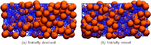
Two simulations of the colloid–polymer mixture are performed independently, one starting from an initial configuration in which pure colloid and polymer phases are brought into contact, and the other starting with a fully mixed system (cf. Figure 2(a) and 2(b), respectively). The aim is to reach a stable phase-separated system starting from opposite extremes, thus establishing proper equilibration. Both systems are first simulated under isobaric–isothermal (NPT) conditions to equilibrate the initial configurations, establishing the appropriate pressure, and then in the canonical (NVT) ensemble; except where stated explicitly, results given correspond to canonical simulations.

Figure 2. Snapshot of the initial configurations in the simulations of the colloid–polymer system: (a) initially demixed and (b) initially mixed systems. To obtain the demixed system, the pure component polymers and colloids are simulated independently before being brought together in a single box. To obtain the mixed configuration, a smaller simulation is initially performed at lower pressure and density; this is then replicated 16 times (twice in x and y and four times in z) to give the configuration illustrated in (b). The pressure is subsequently adjusted to the desired value.

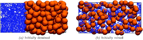
Snapshots of the final configurations with both approaches are presented in Figure 3. Visually, colloid-rich and polymer-rich regions are clearly identifiable, although the system does not appear to be separated into two well-defined bulk regions, with a clearly demarcated interface. This does not necessarily indicate that phase separation has not occurred. For example, it may be that one is unable to stabilise an interface for a system of this size. Estimates have been made of the interfacial width of AO colloid–polymer mixtures. Using density-functional theory, Brader et al. [116] estimated the width to be ∼σ_c close to the triple point while Bryk [55] suggested the width to be a few colloidal diameters wide, and increasing with increasing chain length of the polymer. Vink et al. [79] obtained interfacial widths ∼7–9σ_c using grand canonical Monte Carlo simulation (see figure 3 of reference [79]). Since our simulations are periodic, two interfaces are required in order for the system to stabilise into well-defined colloid-rich and polymer-rich regions. For interfacial widths of ∼5σ_c then even the relatively large system size chosen in our current work will be insufficient to stabilise two phase-separated regions with two corresponding interfaces because the longest side of the simulation cell, 10σ_c, would be no greater than the width of two adjacent interfaces. Moreover, due to the low interfacial tension of colloid–polymer systems, the interfaces are characterised by large local fluctuations not only in width [79] but also in composition [55,79,116]. Accordingly, even when phase separation has occurred, a clear profile of bulk regions separated by an interface is unlikely to be seen for all but the largest systems.

Figure 3. Snapshots of the final configurations of the colloid–polymer system after at least 6.5 × 10⁶ time steps of the simulations: (a) the initially demixed system and (b) the initially mixed system. Visually, both configurations exhibit polymer-rich and colloid-rich regions, suggesting local phase-separated regions.

To establish whether or not phase separation has occurred, careful analysis of the polymer-rich and colloid-rich regions apparent in Figure 3 is required. One cannot simply sample properties along the long (z) axis of the simulation cell, however, since the molecular distributions (polymer and colloid) in the x and y directions within a given sampling volume are no longer uniform. A different approach is required to account properly for these differences in the distribution of the local density of each species. To this end, an algorithm is implemented that is based on the procedure [117] used to sample phase coexistence in systems where the spacial domains of the phases are not fully segregated [118]. In essence, the algorithm consists of sampling the local compositions by randomly analysing small sub-regions of given configurations; a histogram of the local compositions exhibits bimodality if phase separation is present.

We incorporate two important modifications of the procedure to account for the highly asymmetric nature of the colloid–polymer system. In the original scheme [117] one-dimensional profiles are generated by sampling cuboidal sub-systems, randomly distributed in the simulation cell. This is not suitable for use in the study of systems with such a large asymmetry in particle/segment size; the colloid spheres are so large that the diameter of a colloid may be of similar order of magnitude to the width of the sampling volume. A consequence of this is that a sampling volume could contain portions of many colloidal particles, yet be counted as devoid of colloid should none of the colloid centres lie within the sampling volume. Accordingly, using Equation (4(4) $${\eta }_{\mathrm{total}}=\frac{\pi }{6V}\left(N_{\mathrm{c}}{\sigma }_{\mathrm{c}}^3+N_{\mathrm{m}}{\sigma }_{\mathrm{m}}^3\right),$$(4) ) directly (but with V representing the sampling volume) to obtain the local packing fraction leads to unsatisfactory results for the local colloid packing fraction, which is thereby returned as a very noisy function. Here, we adapt the algorithm to account for the portions of the colloids (and only those portions) that lie within the sampling volume, irrespective of where the centres of the colloids lie.

For computational simplicity, spherical sampling volume elements are employed, thus the portion of a colloid to assign to a volume may be calculated as the intersection of two spheres, which is a simple mathematical object referred to as a spherical lens; the volume of a spherical lens depends only of the radii of the spheres and the distance between their centres. The specific procedure employed to calculate the volume of a spherical lens is presented in Appendix A.

A radius of r _samp = 12.5σ_m is chosen for the sampling sphere, based on the best compromise between a large sampling sphere, which more efficiently samples the colloid-rich regions, and a smaller sampling sphere, which more effectively samples the polymer-rich regions. (A discussion of the effect of the sampling-sphere radius on the resulting density distributions is provided in Appendix A.) The analysis is conducted for the last 5 × 10⁵ time steps of each simulation; the resulting probability distributions of the density, $\mathcal{P}\left({\eta }_{\mathrm{total}}\right)$, are displayed in Figure 4. It can be seen that both runs (initially mixed and initially demixed) lead to very similar average density distributions, featuring a sharp peak corresponding to the packing fraction, η^pol _total, of the polymer-rich phase and a broader peak corresponding to the packing fraction, η^col _total, of the colloid-rich phase. This is significant as it indicates that the simulations have converged to configurations with essentially the same density distribution even though, as can be discerned from the snapshots of the initial configurations in Figure 2, the initial density distributions of the two simulations were entirely different.

Figure 4. The average probability distribution, $\mathcal{P}$, of the total packing fraction for the colloid–polymer system with a size ratio of σ_c/σ_m = 20 and polymer length m _p = 100 at the state point corresponding to x _p = 0.67, η_total = 0.28 and P* = 10. The dashed curve represents the initially mixed simulation, while the continuous curve represents the simulation in which polymers and colloids were initially demixed (see Figure 2). The average is accumulated over the last 5 × 10⁵ time steps in each case, using 10⁵ samples per time step, with a sampling-sphere radius of r _samp = 12.5σ_m. The vertical green dashed and red dot-dashed lines represent the densities of the two phases coexisting predicted with the Wertheim TPT1 approach.

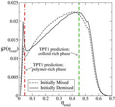
The average distributions obtained from both the initially demixed state and the initially mixed state indicate a total packing fraction of η^pol _total ∼ 0.029 for the polymer-rich phase. Although the peaks corresponding to η^col _total are very broad the maxima are almost coincident at a total packing fraction of η^col _total ∼ 0.43 for the colloid-rich phase. The location of these in relation to the pressure–density phase diagram (Figure 1(b)) is illustrated in Figure 5 (the ‘error bars’ reflect the broad nature of the two peaks, estimated as half their widths at half height). It is interesting to note that the packing fraction of η^col _total ∼ 0.43 is significantly lower than the value of 0.49 where the pure HS system is known to exhibit a transition from a fluid to a solid phase [119].

Figure 5. The simulated values of the packing fraction in the coexisting polymer-rich, ${\eta }_{\mathrm{total}}^{\mathrm{pol}}$ (filled red square), and colloid-rich, ${\eta }_{\mathrm{total}}^{\mathrm{col}}$ (filled green square), phases for the colloid–polymer system with a size ratio of σ_c/σ_m = 20 and polymer length m _p = 100 at the reduced pressure P* = 10. The coexisting packing fractions determined from the two peaks in Figure 4 are seen to coincide closely with the predictions of the Wertheim TPT1 approach (dashed and continuous curves); the ‘error bars’ reflect estimates of the widths of the two peaks (see the text for details). As in Figure 1, the dashed curve represents the polymer-rich phase, the continuous curve represents the colloid-rich phase and the asterisk denotes the critical point of the mixture.

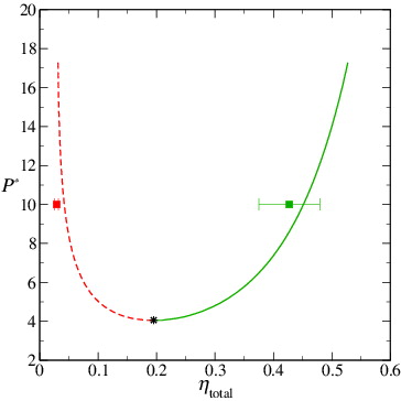
It is striking that the maxima of the average density distributions (i.e., the most-probable densities) obtained from the very different starting configurations coincide closely with the densities of each of the phases (polymer-rich and colloid-rich) calculated using the Wertheim TPT1 approach; note that the positions of these maxima are found to be essentially independent of the sampling-sphere radius employed (see Appendix A). This close correspondence between the theoretical and simulated values is not in line with the findings of Mahynski et al. [71], who obtained a systematic disagreement between coexistence densities for a colloid–polymer system calculated with TPT1 and those obtained in their simulations on a fine-grained lattice. It is important to note, however, that in our current simulations, the polymers are not in the dilute regime (in contrast to those of Mahynski et al.), since the overall packing fraction of even the lower density polymer-rich phase, η^pol _total ∼ 0.029, is in excess of 0.001, the value at which the crossover from dilute to melt behaviour for HS chains is observed [105]. The Flory exponent for swollen HS chains is found to be ν_dilute ∼ 0.60, whereas the exponent for HS chains at η = 0.029 is expected to be ν ∼ 0.53 [105]; this is much closer to the ideal-chain exponent of ν_TPT1 = 0.5 implicit to the TPT1 approach [55]. Moreover, as will be discussed in Section 3.2.2, the polymers behave as though the system is at an effective packing fraction in excess of 0.029, whereby their behaviour will be characterised by an exponent still closer to the ideal-chain value. It may also be significant that Mahynski et al. focused their study on the so-called protein limit, i.e., the regime in which q = R _g/R _c > 1 whereas the mixture examined in our current study lies in the regime corresponding to the colloid limit where q < 1.

The close agreement between the TPT1 predictions and direct simulation obtained in our current work not only provides mutual corroboration of the two approaches, but also lends strong support to the suggestion that phase separation has been achieved in both the initially demixed and initially mixed simulations. Moreover, one can thus be confident that the systems have reached equilibrium, allowing for the fact that (as previously discussed) the size of the system may be too small to allow two well-defined bulk regions separated by clearly demarcated interfacial regions to develop. This confirms that, regardless of the starting conditions (fully mixed or completely demixed), a mixture of our model colloids and polymers at P* = 10 with x _p = 0.65 and η_total = 0.28 is unstable and will phase-separate into a colloid-rich and a polymer-rich phase.

To verify that the phase separation observed is indeed a fluid–fluid separation, the mean squared displacement (MSD) of the colloids is assessed over the final stages of both simulations. Through the last 5.5 × 10⁵ time steps (i.e., ∼8% of the overall length of the simulation), the MSD is found to increase linearly with time. Moreover, the colloids have moved (on average) more than 20 times their diameter during the course of the simulation. One can therefore conclude that the colloids are behaving as a fluid in each phase, and that neither a solid nor a glassy state has been formed. This conclusion will be confirmed by the additional analysis provided in the next section.

Before moving on to discuss our examination of the individual phases, it is interesting to analyse our two-phase system in terms of the interfacial tension that is implicit from the information accrued thus far, and to make comparisons with existing work. Adopting the approach of Binder [120–122] the interfacial tension γ of our two-phase colloid–polymer system can be estimated from the height $\Delta \mathcal{P}$ of the peaks in the probability distributions of the density (measured relative to the ‘interfacial’ states), which is related to the surface free energy F _surf and interfacial tension through (5) $$\gamma =\frac{F_{\mathrm{surf}}}{\mathcal{A}}\sim \frac{-k_{\mathrm{B}}Tln\left(\Delta \mathcal{P}\right)}{\mathcal{A}},$$(5) where $\mathcal{A}$ represents the area of the interface. From Figure 4 we estimate $\Delta \mathcal{P}\sim 0.01$, and we take $\mathcal{A}\sim 25{\sigma }_{\mathrm{c}}^2$, corresponding to the smallest cross section of our simulation box. We thus obtain an estimate of the dimensionless interfacial tension as (6) $${\gamma }^{*}=\frac{\gamma {\sigma }_{\mathrm{c}}^2}{k_{\mathrm{B}}T}\sim 0.18.$$(6) Moncho-Jordá et al. [52] used square-gradient theory to compute the interfacial tension for systems of colloids with interacting and non-interacting polymers in a good solvent. In their figure 4, these authors provide values of the interfacial tension as a function of the difference Δη in the packing fraction of the two phases, and the polymer/colloid size ratio q. From this figure, one can read off γR ² _c/(k _B T) ∼ 0.05 (where R _c is the colloid radius) for Δη ∼ 0.41 and q = 0.6 (corresponding to the system in our current work; see Section 3.2.2 for our estimate of q ∼ 0.6), which yields an interfacial tension of γ* ∼ 0.2, in remarkably good agreement with our estimate of γ* ∼ 0.18.

To make a comparison with an experimental system, one first needs to define a length scale. Aarts et al. [123] studied the free fluid–fluid interface in a phase-separated colloid–polymer dispersion using laser scanning confocal microscopy. The size of the colloids was measured as σ_c = 142 nm, and the size ratio q = 0.6, the same as in our current study. Using σ_c = 142 nm to define a length scale for our simulations, and assigning an ambient temperature (T ∼ 300 K), our simulated interfacial tension corresponds to γ ∼ 40 nN m⁻¹, which is in order-of-magnitude agreement with the ultra-low interfacial tensions reported in reference [123]. The agreement we obtain with this study (and the theoretical work of Moncho-Jordá et al. [52]) not only further supports the conclusion that our colloid–polymer mixture is indeed phase-separated, but also adds further insight into the absence of a clearly defined interface in our simulations. Aarts et al. [123] were able to directly observe thermal capillary waves in their study; from their figure 2, the amplitudes and wavelengths of the capillary waves can be seen to be of the order of a few microns, corresponding to a few tens of colloid diameters. Recalling that the longest dimension of our simulation cell is 10σ_c, one can thereby again conclude that a very much larger simulation cell would be required in order to stabilise a well-defined interface between the two phases.

3.2.2. Studies of the separate polymer-rich and colloid-rich phases

To properly understand the colloid–polymer system in terms of its structural and thermodynamic behaviour, it is useful to examine each of the coexisting phases separately. Based on the evidence provided by the probability distribution of the density (cf. Figure 4(b)) and quantified in Figure 5, we henceforth assume that the two phases exactly match the theoretical predictions from TPT1 [59] and, accordingly, the density and composition of each phase are taken to be those indicated by TPT1 (see Figure 1(a) and 1(b)). (Although this assumption results in very slightly higher densities in each phase than those indicated by the peaks of the distributions in Figure 4, one thereby avoids possible complications arising from the statistical uncertainty in the compositions of the two phases that stems from the small number of colloids present in the simulation.) Using this information, separate cubic simulation boxes are constructed, each representing one of the two phases; details are given in Table 1. Simulations of each phase are performed in the canonical (NVT) ensemble.

Table 1. Details of the simulations of the separate polymer-rich and colloid-rich phases as predicted with the TPT1 approach for the colloid–polymer system with a size ratio of σ_c/σ_m = 20 and polymer length m _p = 100 at the reduced pressure of P* = 10; L is the length of the (cubic) simulation cell.

						Total number of sites
System	${\eta }_{\mathrm{total}}$	L/σc	x p	N c	N p	(N c + N p m p)
Polymer-rich phase	0.0427	5.41	0.980	8	392	39,208
Colloid-rich phase	0.4581	10.46	0.111	1000	125	13,500

To examine the dimensions of the polymers, we calculate their average radius of gyration, R _g, in each of the two phases. R _g is defined as the root-mean-square distance of the monomers from the centre of mass (CoM) of the chain: (7) $$R_{\mathrm{g}}^2=\frac{1}{m_{\mathrm{p}}}\sum _{i=1}^{m_{\mathrm{p}}}{\left({\mathbf{r}}_i-{\mathbf{R}}_{\mathrm{CoM}}\right)}^2.$$(7) The sum is over the entire chain length of the polymer m _p (in the current work m _p = 100 segments); R _CoM represents the position of the centre of mass of the chain (assuming all segments have the same dimensionless mass), and is given by (8) $$R_{\mathrm{CoM}}=\frac{1}{m_{\mathrm{p}}}\sum _{i=1}^{m_{\mathrm{p}}}{\mathbf{r}}_i,$$(8) and r _i similarly represents the position of the ith segment.

The probability distributions obtained for the radii of gyration are presented for the polymer-rich and the colloid-rich phases in Figure 6. Both distributions exhibit a peak at R _g/σ_m ∼ 6, so that the size ratio for our system is q = R _g/R _c ∼ 0.6. One can discern from Figure 6 that the difference between the most-probable R _g values of the polymer in the two phases is less than 6%. It is important to note that, although this difference is small, this does not mean that the structure of the polymers in the two phases will be similar. Indeed, the similarity in the dimensions of the polymers may itself seem a surprising result, considering the difference in the packing fractions of the polymer-rich (η^pol _total = 0.0427) and the colloid-rich phase (η^col _total = 0.4581). Even though the overall packing fraction of the colloid phase is only ∼3% lower than the value at which pure HSs undergo a liquid–solid transition, this suggests that the polymers are able to occupy the interstitial regions, which are relatively large empty regions when compared to the volume occupied by the monomers.

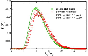
Figure 6. Comparison of the probability distributions of the polymer radius of gyration for the separate polymer-rich (red diamonds) and colloid-rich (green circles) phases for the colloid–polymer system with a size ratio of σ_c/σ_m = 20 and polymer length m _p = 100 at the reduced pressure P* = 10. The symbols represent the values obtained during simulations of the mixture. The curves represent the distributions obtained from simulations of the equivalent pure (one-component) polymer systems; the continuous green curve represents simulations at a packing fraction η_p = 0.075, while the red dashed curve represents data corresponding to a packing fraction of η_p = 0.05.

An order-of-magnitude calculation of the relative volumes involved is helpful. In the close-packed limit, in which the colloids form a tightly packed fcc lattice, the packing fraction is η_fcc = 0.74; in other words 26% of the space is free. In an fcc unit cell with four colloids, given that σ_c = 20σ_m, there is an empty volume equivalent to that of 496 monomeric segments of the polymer. In the colloid-rich phase the ratio of polymers to colloids is 1/8 (see Table 1), so the number of polymers that would correspond to four colloids is ∼0.5, comprising ∼50 monomers. In other words, even in the case of close-packed colloidal particles, there would be space for ∼50 monomers in a unit cell; of course, the actual density of the colloids is substantially lower than that of a close-packed system, with even more volume available to the polymers. Using Equation (4(4) $${\eta }_{\mathrm{total}}=\frac{\pi }{6V}\left(N_{\mathrm{c}}{\sigma }_{\mathrm{c}}^3+N_{\mathrm{m}}{\sigma }_{\mathrm{m}}^3\right),$$(4) ) but replacing V with the empty volume that has just been discussed, a ‘local’ polymer packing fraction of η_{p, local} = 0.013 would be obtained. However, the polymers and colloids share the same space and the colloids are not stationary, so such a calculation is rather crude. In reality, the polymers behave as though the system is at an effective packing fraction which will be higher than η_{p, local} = 0.013 but much less than η^col _total = 0.4581.

It has been shown that for (pure) HS polymer chains of degree 50 ≤ 2000 the crossover from the swollen (dilute) to the melt regime takes place between η ∼ 0.001 and η ∼ 0.17 [105]. If the effective packing fraction of the polymers in the colloid–polymer mixture lies within this interval, then one way to establish its value is to perform simulations of pure polymers at varying packing fractions in this range, comparing the probability distributions of the dimensions obtained from these simulations with those of the mixture. Accordingly, also displayed in Figure 6 are distributions obtained from the simulation of the corresponding pure- polymer systems at packing fractions η_p = 0.05 and η_p = 0.075. Gratifyingly, the former lies close to the data corresponding to the simulation of the polymer-rich phase of the colloid–polymer mixture, for which the packing fraction η^pol _total = 0.0427, but centred on a slightly smaller value of R _g, consistent with the slightly higher packing fraction of the pure-polymer simulation. The distribution obtained from the simulation at η_p = 0.075 coincides quite closely with the data corresponding to the simulation of the colloid-rich phase of the mixture, indicating that the polymers in this phase behave as though the system is at an effective packing fraction close to, but a little below this value.

Frenkel [124] has pointed out that hard-core spherical particles with an attractive range spanning less than 20% of their diameter do not exhibit a stable vapour–liquid transition, since the vapour–liquid critical point drops below the triple point. This concurs with the ‘rule of thumb’ for the depletion interaction between colloids in colloid–polymer mixtures, prescribed by Likos [32], that when the range of attraction is more than 20% of the range of the repulsive cores, the liquid phase is stable and the phase diagram features two fluid phases and one solid phase; such behaviour has been seen experimentally, e.g., by Calderon et al. [3]. For polymers in the swollen (dilute) regime, one would expect that the thickness of the depletion layer around the colloids is close to R _g and that the range of the depletion interaction for our system is ∼2R _g = 12σ_m = 0.6σ_c.[1,125] This would correspond to a range of the attractive depletion well which is in excess of the threshold value (∼σ_c/5), below which the colloidal liquid phase is expected to become metastable relative to the solid [124]. However, since the effective polymer packing fraction corresponds to the crossover (or semi-dilute) region between swollen chains and the melt, the range of the depletion interaction is determined not by R _g but, rather, by a correlation length ξ, often referred to as the blob size of the polymer [33,125–127]. Using information pertaining to the dimensions of HS polymer chains (see table III of reference [105]) together with a simple scaling argument [105], the blob radius ξ of the 100-segment HS polymer chains at η_p = 0.075 can be estimated to be of the order of 3σ_m to 4σ_m, whereby the range of the interaction would be approximately 6σ_m to 8σ_m $\gtrsim$ σ_c/3 (see Appendix B for a description of the scaling argument). This value still exceeds the theoretical threshold below which the liquid phase is expected to be metastable, and corresponds to a depletion thickness to colloid radius ratio of q _s ∼ 0.3–0.4. The phase diagram for a system with this value of q _s may be expected to correspond roughly to that provided in figure 1.1 of reference [34], which features ‘gas–liquid’, ‘gas–solid’ and ‘fluid–solid’ phase boundaries. It is noticeable that the solid phase is characterised by η_c $\gtrsim$ 0.54, corresponding to the well-known coexistence packing fraction for pure HS, and significantly in excess of the total packing fraction (polymers + colloids) of the denser of the two phases we find in our simulations. One can also discern that the packing fractions of the liquid phase along the gas–liquid binodal lie between η_c ∼ 0.27 (at the critical point) and η_c ∼ 0.46 (at the triple point), spanning our value of η_total ^col = 0.4581 for the colloid-rich phase. Taken together, these observations provide strong corroboration of our earlier conclusion that the phase transition we observe is fluid–fluid, and not fluid–solid in nature.

It is known that HS chains in simulations of pure polymers at densities corresponding to those of our current work (η_p = 0.05 and η_p = 0.075) are not, on average, extended so that polymers behave as though spherical [105,128]. The close coincidence between the distributions relating to the pure polymers and those relating to the corresponding simulations of the colloid–polymer mixture suggests that, on average, the polymers in the mixture are also spherical and not extended, even in the colloid-rich phase. This implies that although the polymer chains are mutually interpenetrable, effectively they behave as spherical entities that are almost impenetrable by the colloids – rather in the spirit of the AO model. This is a helpful conclusion as it implies that one may usefully probe the structure of the fluid phases using molecular distribution functions of the CoM.

The radial distribution function, g(r), is defined as the ratio of the local number density of particles or molecules from a central particle to the bulk number density, ρ. It may be evaluated as [129] (9) $$g\left(r\right)=⟨\frac{n\left(r\right)}{\rho \pi r^2\delta r}⟩,$$(9) where n(r) is the number of particles in a shell bounded by the distances r and r + δr from the given particle, and the angular brackets represent the ensemble average over all particles. The internal structure of the two phases is presented in Figure 7 in the form of the colloid–colloid, g _cc(r), colloid–polymer, g _cp(r), and polymer–polymer, g _pp(r), radial distribution functions; the colloid-rich phase is represented in (a), and the polymer-rich phase in (b).

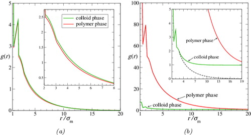
Figure 7. The molecular (centre-of-mass) pair radial distribution functions in (a) the colloid-rich phase (colloidal ‘liquid’) and (b) the polymer-rich phase (colloidal ‘gas’) for the colloid–polymer system with a size ratio of σ_c/σ_m = 20 and polymer length m _p = 100 at the reduced pressure P* = 10. The continuous green curves represent the colloid–colloid g _cc(r), the black curves represent the colloid–polymer g _cp(r), and the red curves represent the polymer–polymer g _pp(r). Vertical dashed lines correspond to σ_c, σ_p, and σ_cp = (σ_c + σ_p)/2; the effective diameter of the polymer, σ_p, is calculated as twice the average radius of gyration for each phase. (The scales on the axes are expanded in (b).)

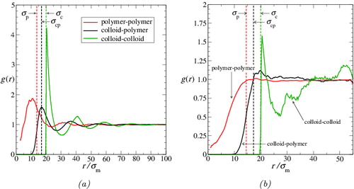
As one might expect, the colloid–colloid distribution function g _cc(r) in the colloid-rich phase (the green curve in Figure 7(a)) is beautifully characteristic of a dense liquid phase comprising HSs of diameter σ_c. Due to the small number of colloids in the polymer-rich phase the statistics relating to the colloids in this phase are poor (to keep the simulation tractable, the simulation contains only eight colloids). Consequently, g _cc(r) is too noisy to draw any firm conclusions about the behaviour of the colloids in this phase.

We consider next the colloid–polymer distribution function g _cp(r). In the colloid-rich phase (cf. Figure 7(a)), g _cp(r) has its first peak almost exactly at σ_cp = (σ_c + σ_p)/2, with subsequent weaker peaks at 2σ_cp and 3σ_cp, just as one would expect for a liquid-like radial distribution function for mixtures of spheres of diameter σ_p and σ_c. This corroborates the earlier conclusion that the polymers behave as spherical entities from the perspective of the colloids. Moreover, the location of the first peak at σ_cp is a further indication of the relative impenetrability of the polymers to the colloids. The widths of the peaks provide an indication of the relative softness or hardness of the colloid–polymer interaction; although broader than those of g _cc(r), it is interesting to note that the peaks are nevertheless quite sharp. In the polymer-rich phase (cf. Figure 7(b)) g _cp(r) is rather noisy. Even so, it is consistent with a low-density vapour-like radial distribution function for mixtures of spheres of diameter σ_p and σ_c, once again supporting the earlier interpretation that the colloids effectively ‘see’ the polymers as spherical particles.

The different forms of the polymer–polymer distribution function g _pp(r) in the two phases are of particular interest. As expected, g _pp(r) is essentially liquid-like in the colloid-rich phase. However one can see clear evidence of interpenetration of the polymer spheres. This is indicated firstly by the trend of g _pp(r) as r approaches zero; for impenetrable spheres, g(r) would be zero for r < σ_p, whereas g _pp(r) remains non-zero within the polymeric core. The next indicator is that the first major peak does not appear exactly at σ_p (as would be the case for fully impenetrable spheres) but, rather, at a slightly smaller value of r; the displacement of the first peak alone reflects that the interpenetration of the soft polymer spheres occurs (by its nature) at small inter-polymer separations. All of the peaks in g _pp(r) are broader (and noisier) than the corresponding peaks in g _cc(r) or g _cp(r); this is consistent with a softer intermolecular interaction between the polymers than that between polymers and colloids, and that between colloids. In the polymer-rich phase, g _pp(r) has a form somewhat characteristic of a ‘vapour’ state. Once again, there is evidence of interpenetration of the spherical polymeric cores since, as in the colloid-rich phase, g _pp(r) remains non-zero at values of r substantially lower than the ‘contact distance”, σ_p = 2R _g.

The radial distribution function can be related to the potential of mean force, ω, via the expression ω(r) = −k _B T ln g(r). Accordingly, one can extract information relating to the average interactions between the particles from the appropriate radial distribution functions; indeed, in the low-density limit ω tends to the effective pair potential between particles. Since our simulations are not carried out at low densities, a rigorous approach such as that followed by Bolhuis et al. [74] should, strictly speaking, be used to extract the effective pair potentials from g(r) in our simulations. Bolhuis et al. solved the Ornstein–Zernicke [130] equation with the hypernetted-chain closure [131] using a self-consistent iterative procedure to obtain effective CoM–CoM pair potentials for their lattice-model polymers. In our current work, we seek only to examine the general features of the interactions, so an examination of the potential of mean force is sufficient.

In Figure 8 we display the potentials of mean force relating to the colloid–colloid, colloid–polymer, and polymer–polymer interactions extracted from the corresponding g(r) plots displayed in Figure 7. The colloid–colloid ω_cc(r) within the colloid-rich region is characterised by a deep trough at σ_c: this indicates the expected (depletion-induced) effective attractive interaction between the colloids. The statistics are too poor to extract a meaningful ω_cc(r) effective interaction for the polymer-rich phase. Although less pronounced, there is also a clear well in the colloid–polymer ω_cp(r) in the colloid-rich phase, indicating an effective attraction between the polymers and the colloids. Perhaps most surprising is that there is also a deep trough in the polymer–polymer ω_pp(r) in the colloid-rich phase, similarly indicating that an effective attraction exists between the polymer molecules in this phase. It appears from these observations that the depletion interaction is not restricted to the colloids; the presence of polymer molecules not only results in a depletion interaction between the colloids but, in concert, the presence of the colloids appears to induce a depletion interaction between the polymers.

Figure 8. Potentials of mean force, ω(r), extracted from the radial distribution functions displayed in Figure 7 for the colloid–polymer system with a size ratio of σ_c/σ_m = 20 and polymer length m _p = 100 at the reduced pressure P* = 10. The potentials relating to the colloid-rich phase are given in (a), while those relating to the polymer-rich phase are given in (b). The continuous green curves represent the colloid–colloid ω_cc(r), the black curves represent the colloid–polymer ω_cp(r), and the red curves represent the polymer–polymer ω_pp(r). Note that the statistics are too poor to extract ω_cc(r) for the polymer-rich phase.

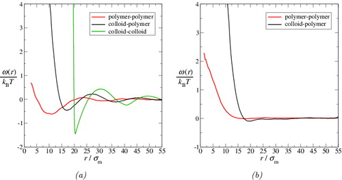
By contrast, in Figure 8(b), there is no clear evidence of an effective attractive interaction between the molecules, although one can perhaps discern a small well in ω_cp(r) at r just greater than σ_cp. The differences between the potentials of mean force displayed in (a) and (b) clearly indicate that both the colloid–polymer and polymer–polymer interactions in the colloid-rich phase differ significantly from their respective counterparts in the polymer-rich phase. This is a particularly interesting conclusion in relation to the effective polymer–polymer interaction, considering the apparent similarity in the dimensions of the polymers in the two phases (cf. Figure 6). Such a difference in the effective interactions between the polymer chains in the two phases is not generally taken into account in theoretical treatments of colloid–polymer systems.

It is interesting to compare our ω_pp(r) with the effective CoM intermolecular potentials obtained by Bolhuis et al. [74] in their lattice simulations of self-avoiding-walk polymers. To facilitate comparison with reference [74], and to highlight the difference between the polymer–polymer interactions in the two phases, ω_pp(r) for each phase is plotted again in Figure 9, though here normalised relative to the radius of gyration of the polymer in the corresponding phase.

Figure 9. The potentials of mean force, ω_pp(r), corresponding to the polymer–polymer interaction in the colloid-rich and polymer-rich phases, normalised relative to the corresponding radius of gyration, for the colloid–polymer system with a size ratio of σ_c/σ_m = 20 and polymer length m _p = 100 at the reduced pressure P* = 10. The continuous green and red curves correspond to the colloid-rich and polymer-rich phases, respectively, while the dashed and dot-dashed black curves correspond to effective CoM–CoM potentials obtained by Bolhuis et al. [74] from their lattice simulations; the former corresponds to the potential between isolated chains of 100 segments, and the latter to chains of 500 segments in the semi-dilute regime at a density corresponding approximately to the effective packing fraction of polymers in the colloid-rich phase of our current simulations.

Also given in the figure are two of the effective CoM–CoM potentials obtained by Bolhuis et al. [74] from their lattice simulations. One corresponds to the potential between isolated chains of 100 segments, and another to chains of 500 segments in the semi-dilute regime at a density corresponding approximately to the effective packing fraction of polymers in the colloid-rich phase of our current simulations. For consistency with these simulations, one might expect our results to lie approximately between these two curves. In the polymer-rich phase ω_pp(r) ∼ 2k _B T at r ∼ 0, dropping smoothly to zero at r ∼ 2 to 3 R _g; this is indeed consistent with the effective CoM–CoM potentials of reference [74]; interestingly, along much of its length our curve almost superimposes with that corresponding to the isolated 100-segment chains. However, the behaviour of ω_pp(r) in the colloid-rich phase is in stark contrast to the curves obtained by Bolhuis et al. [74].

One can further probe the polymer behaviour by looking at the site–site (colloid–colloid, colloid–monomer, and monomer–monomer) radial distribution functions. The site–site radial distribution functions obtained from our MD simulations of the colloid-rich and polymer-rich phases are presented in Figure 10; note that since the colloids are modelled as single spheres, the colloid–colloid functions represented here are identical to the molecular g _cc(r) of Figure 7. In addition, for comparison, distribution functions relating to simpler HS systems are also included in the figures: $g_{{}_{\mathrm{HS}}}\left(r\right)$ of a pure (one-component) system of diameter σ_c at the same packing fraction as the mixture; binary HS mixture of large and small spheres corresponding to the colloid–monomer $g_{\mathrm{cm},{\mathrm{HS}}_{\mathrm{mix}}}\left(r\right)$ and colloid–colloid $g_{\mathrm{cc},{\mathrm{HS}}_{\mathrm{mix}}}\left(r\right)$ cases. The HS mixture mimics the colloid–polymer mixture except that the monomer HS segments comprising the polymer are not connected (i.e., the mixture comprises simply large HS of diameter σ_c and small HS of diameter σ_m); it thus has (by construction) the same density and (segment) composition as the phase of the actual mixture.

Figure 10. Site–site pair radial distribution functions in (a) the colloid-rich and (b) the polymer-rich phases for the colloid–polymer system with a size ratio of σ_c/σ_m = 20 and polymer length m _p = 100 at the reduced pressure P* = 10, compared with those for equivalent HS systems at the same density. Broken curves represent binary HS mixtures of the same density and (segment) composition as the phase (i.e., comprising the same numbers of HS colloids and (unconnected) HS polymer monomer segments; see text for details). The continuous curves represent the colloid–polymer systems; the green curves indicate colloid–colloid g _cc(r) (reproduced from Figure 7) and the violet curves indicate colloid–monomer g _cm(r). For clarity, the curves representing g _cm(r) are shifted up by unity. The filled grey circles indicate $g_{{}_{\mathrm{HS}}}\left(r\right)$ of a pure (one-component) system of HSs of diameter σ _c at the same packing fraction, η_total, of the phase.

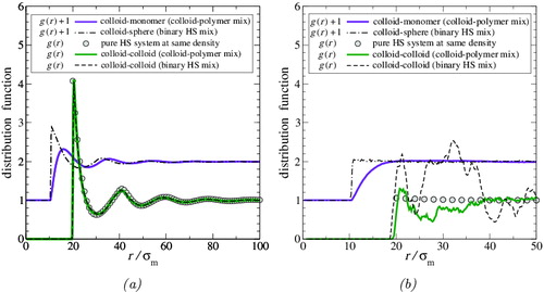
It is evident from Figure 10(a) that the presence of the monomers, whether unconnected or joined into polymer chains, has almost no influence on the structure of the colloids in the colloid-rich phase, since g _cc(r) for this phase coincides almost exactly with both $g_{\mathrm{cc},{\mathrm{HS}}_{\mathrm{mix}}}\left(r\right)$ and $g_{{}_{\mathrm{HS}}}\left(r\right)$. Although this is consistent with the earlier conclusion that the polymers occupy interstitial regions between the colloids, it is still a surprising result, since it appears to indicate that any depletion interaction experienced by the colloids is, at most, weak. It is interesting, in particular, to draw attention to the especially close match of g _cc(r) and $g_{\mathrm{cc},{\mathrm{HS}}_{\mathrm{mix}}}\left(r\right)$. Hitherto, we have given no consideration to the so-called ‘depletion stabilisation’ phenomenon: under certain conditions, the depletion layer can give rise to an effective repulsive interaction between the colloids. Shvets and Semenov [92] have suggested that the nomenclature ‘depletion stabilisation’ is misleading, preferring the term ‘long-range free polymer induced’ (FPI) repulsion. These authors have shown that while one expects only the classical polymer-mediated depletion attractive interactions when the polymers are in the dilute (swollen) regime, an FPI repulsion may be expected for colloid surface–surface separations in excess of 10ξ, when ξ $\gtrsim$ 0.5R _g. Recalling our earlier estimate of ξ ∼ 3σ_m to 4σ_m and that R _g $\gtrsim$ 6σ_m, one might therefore expect to see some evidence of an FPI repulsion in our simulations at colloid separations in excess of 30σ_m. On close inspection of g _cc(r) one does indeed see that the first trough in the distribution, at ∼30σ_m, is indeed shifted marginally to longer r in comparison to $g_{{}_{\mathrm{HS}}}\left(r\right)$; this is reflected in the potential of mean force (cf. Figure 8), with a peak at r slightly in excess of 30σ_m, and one could easily be misled into interpreting these observations as evidence of an FPI repulsion interaction. However, the almost exact coincidence of g _cc(r) and $g_{\mathrm{cc},{\mathrm{HS}}_{\mathrm{mix}}}\left(r\right)$ demonstrates that this cannot be the case; the origin of the FPI repulsion is a chain-end effect [92] whereas, from this comparison, one can quite clearly see that there is no impact of any sort of chain connectivity on the structure of the colloidal fluid.

Although the structural influence on the colloids is negligible, that on the monomers is not. This is shown by the disagreement at short range between g _cm(r) and $g_{\mathrm{cm},{\mathrm{HS}}_{\mathrm{mix}}}\left(r\right)$, indicating that the connectivity of the segments constrains the manner in which they order in the vicinity of the colloids; evidently the connected segments do not fill so closely the space between the colloids as unconnected HS of the same diameter. A similar short-range effect is manifest relating to these two functions in the polymer-rich phase, illustrated in (b). Unfortunately, as already discussed, due to the necessarily small size of the system there are insufficient colloids present in the polymer-rich phase to provide good statistics, so that the distribution functions in (b) are rather noisy. There is a pronounced difference between g _cc(r) and the colloid–colloid $g_{\mathrm{cc},{\mathrm{HS}}_{\mathrm{mix}}}\left(r\right)$ of the binary HS mixture, while neither coincides closely with $g_{{}_{\mathrm{HS}}}\left(r\right)$ from the pure-HS simulation. Accordingly, it is tempting to conclude not only that the presence of the monomers influences the structure of the colloids in this phase, but also that the connectivity of the monomers into chains is important. This would be consistent with the earlier conclusion that, effectively, the polymer behaves as spheres that are almost impenetrable by the colloids. However, one cannot rule out the possibility that the differences are due to no more than noise.

As the final component of this analysis, we examine the site–site distribution functions relating to the monomers comprising the polymer chains; monomer–monomer distribution functions for the colloid-rich and polymer-rich phases are presented in Figure 11. The features in these curves are dominated by the connectivity of monomers belonging to the same chain. This gives rise to a δ function at r = σ_m, which is manifest in the figures as an extremely sharp peak (the height and width of which are determined by the bin size used in the accumulation of the statistics). A second peak appears at r = 2σ_m, and there is a further discontinuity in the gradient at r = 3σ_m, after which the function decays smoothly. These features are clearly discernible in Figure 11(a), in which g _{mm, internal}(r) is displayed. Only monomers belonging to the same chain are counted in the accumulation of g _{mm, internal}(r); accordingly the function decays to zero (rather than unity), at r ∼ σ_p (σ_p ^pol ∼ 14.5σ_m for the polymer-rich phase; σ_p ^col ∼ 13.8σ_m for the colloid-rich phase). One can discern a small but clear difference in the structure of the chains in the two phases at short r, as is highlighted by the inset in the figure; g _{mm, internal}(r) is systematically larger in the colloid-rich phase. However, the internal structure of the chain for r $\gtrsim$ 10σ_m appears to be almost identical regardless of the phase.

Figure 11. Monomer–monomer radial distribution functions of the polymers in both phases for the colloid–polymer system with a size ratio of σ_c/σ_m = 20 and polymer length m _p = 100 at the reduced pressure P* = 10: (a) internal monomer distribution g _{mm, internal}(r) for segments on the same chain; and (b) overall monomer distribution g _mm(r). The green curves represent results for the colloid-rich phase while the red curves correspond to those of the polymer-rich phase. The dashed black curve in the inset of (b) represents the internal monomer distribution for the colloid-rich phase (i.e., the green curve from (a)); comparison of this curve with the overall distribution reveals the extent of interpenetration of the polymer chains in this phase (see the text for a discussion). The separation of the green and red curves in (b) indicates that the polymer chains in the polymer-rich phase interpenetrate far more than those in the colloid-rich phase.

In Figure 11(b) the overall g _mm(r) is also presented; this function takes into account all of the monomer segments, regardless of whether or not they belong to the same chain. The features of these curves are still dominated by chain connectivity; they exhibit qualitatively similar characteristics to those in (a). However, one can discern from (b) that g _mm(r) in the polymer-rich phase remains above unity well in excess of r = σ_p (see the inset graph in (b)); this indicates local ‘clustering’ of polymer molecules in the polymer-rich phase, as one might intuitively expect given that the polymer chains interpenetrate. In addition, the plots in (b) reveal further information concerning the interpenetration of the polymer molecules. The difference seen between the curves in the polymer-rich and colloid-rich phases is partly due to the difference in the densities of polymers in the two phases. However, the considerable separation of the two curves at short r (i.e., r < R _g) demonstrates that there is considerably more interpenetration of the chains in the polymer-rich phase than in the colloid-rich phase. This is to be expected, since the density of polymers in the polymer-rich phase is much higher than that in the colloid-rich phase.

That there is, nevertheless, interpenetration of chains in the colloid-rich phase is confirmed by comparing g _mm(r) in (b) with its counterpart g _{mm, internal}(r) in (a); for convenience, the tail of the latter is reproduced in the inset as the black dashed curve. The difference between the two curves at r $\gtrsim$ σ_p is due to monomers from other chains penetrating the chain to which the reference monomer segment belongs. Interpenetration of chains also explains why g _mm(r) reaches its asymptotic value of unity well before σ_p.

Altogether, the information in Figure 11 reveals that the internal structure of the polymer chains in the two phases is quite similar (thereby providing some enlightenment into the success of simple theoretical approaches, such as that of Asakura and Oosawa [29]) but that there are important differences which are manifest in the different degrees of interpenetration of the polymers in the two phases; the presence of the colloid molecules in the colloid-rich phase influences the penetrability of the polymers by each other.

4. Discussion and conclusions

Using MD simulation we have successfully demonstrated fluid-phase separation in a model colloid–polymer system comprising HS polymer chains (formed from 100 tangentially bonded HS segments) and HS colloids with a diameter 20 times that of the polymer segments. The system is found to exhibit coexistence between a colloid-rich phase and a polymer-rich phase. Under the conditions of our simulations, the radius of gyration of the polymers is ∼6 monomer diameters, so that the size ratio q = R _g/R _c ∼ 0.6, whereby our system lies at the so-called colloid limit (q < 1). The densities of the two phases are in accordance with predictions made using Wertheim's TPT1; this agreement between the simulation and TPT1 provides mutual corroboration of each approach. A useful outcome of the theoretical predictions is an identification of the compositions of the two coexisting phases, particularly that of the low-density polymer-rich phase. Although this information is also available from the simulations, the statistical uncertainty associated with the simulated value of the composition of the polymer-rich phase is inevitably high due to the small number of colloids present.

While TPT1 provides no insight at the molecular level, the molecular simulations allow one to probe the structure of the fluid mixture and, thereby, develop insight into the effective interactions between the species in the mixture. Our detailed examination of the two coexisting phases has been especially revealing. Various indicators, such as the molecular (CoM) colloid–polymer distribution function, g _cp(r), suggest that as expected, from the point of view of the colloids, the polymers behave (on average) as soft, impenetrable spheres of radius σ_cp ∼ (σ_p + σ_c)/2. The polymers are interpenetrable by each other, as can clearly be seen from both the polymer–polymer and monomer–monomer distribution functions, g _pp(r) and g _mm(r). The latter further reveal that the interpenetration is greater in the polymer-rich phase; this is intuitively sensible since the density of polymers in this phase is higher. Comparing the colloid–colloid distribution function (g _cc(r)) with the analogous function ($g_{{}_{\mathrm{HS}}}\left(r\right)$) accumulated in a simulation of pure HSs (colloids) surprisingly reveals that the structure of the fluid with respect to the colloids is virtually unaffected by the presence of the polymers, indicating that any depletion interaction between the colloids due to the presence of the polymers is rather weak. However, the presence of the colloids does affect the structure of the polymer molecules. Based on an analysis of the polymer dimensions, the polymers in the colloid-rich phase behave as though the polymers are at an effective packing fraction of η_p ∼ 0.075, although the actual polymer density in this phase is much lower. This effective density is higher than the density of the polymer-rich phase. The interpenetration of polymer molecules would be expected to increase with density in systems of pure polymer whereas, as already noted, the interpenetration of polymers in the colloid-rich phase is demonstrated by analysis of g _mm(r) to be lower than that in the polymer-rich phase. The increase in effective density, allied to a decrease in interpenetration, demonstrates that the structure of the polymers is affected by the colloids. Denton and co-workers have performed simulation studies of crowding of polymer coils in mixtures with nanoparticles in the colloid [132] and the protein [91] limits. These authors observed that polymer coils, modelled as effective penetrable ellipsoids, both contracted and (in the protein limit) became more spherical when crowded by impenetrable, spherical nanoparticles. The analysis in our current study precludes any assessment of possible change in the relative sphericity of the polymer chains brought about by the presence of the colloids; however, the high effective density of the polymers we observe in the colloid-rich phase is consistent with the compaction of the polymer coils observed by Denton and co-workers.

Radial distribution functions are closely related to potentials of mean force and, thereby, provide information relating to the effective interactions between molecules in the low-density limit. The interactions between polymers in the polymer-rich phase are seen to be consistent with the effective potentials obtained in previous work [74]; however, the analogous interactions in the colloid-rich phase turn out to be entirely different, featuring a region of effective attraction between the polymer chains that is absent in the polymer-rich phase. This could, perhaps, be evidence of a depletion interaction between the polymers; such an interpretation is strengthened by an analysis of the interaction between polymers in a pure-polymer simulation at the effective packing fraction η_p ∼ 0.075, where no evidence of attraction is seen. Based on our other observations, the difference between the polymer–polymer interaction in the two (colloid-rich and polymer-rich) phases may be due to the manner in which the colloids affect the interpenetration of the polymer molecules.

It is widely regarded that the physics of the colloid limit is now well understood [56,89–91] (although various authors have recently highlighted some shortcomings in the current understanding [35,92,94]). However, in theoretical treatments of colloid–polymer systems, it is usual to assume that the effective interaction between polymers is the same at the different thermodynamic states, even when going beyond a simple AO treatment. It is clear from our study that this assumption is not necessarily valid, although the importance of this is not clear since a good representation of colloid--polymer systems have been obtained without taking account of the observed difference between the polymer–polymer interactions in colloid-rich and polymer-rich environments. For example, in simulations using their coarse-grained potential [74] to represent the polymer–polymer interaction, Bolhuis et al. [77] obtained excellent agreement with the experimental volume-fraction (φ_c vs. φ_p) phase diagram of a colloid–polymer system with a size ratio of σ_p/σ_c = 0.67. Although their potential is (weakly) density dependent, it was obtained from earlier bulk simulations of self-avoiding-walk polymers with no colloids present and, thereby, cannot take into account any influence of the colloids on the effective polymer–polymer interaction such as that uncovered in our current work. Accordingly, the incorporation of a more representative polymer–polymer interaction into a theoretical approach, allowing for the difference between colloid-rich and polymer-rich phases, would be very interesting.

Acknowledgements

J. Jover and A.J. Haslam gratefully acknowledge The Engineering and Physical Sciences Research Council (EPSRC) of the United Kingdom for funding a PhD studentship and a Research Fellowship, respectively (grant EP/D503051). Additional support to the Molecular Systems Engineering Group from the EPSRC (grants EP/E016340 and EP/J014958), the Joint Research Equipment Initiative (JREI) (GR/M94426), and the Royal Society-Wolfson Foundation refurbishment scheme (RSWF/SUC11/RND3/EEP) is gratefully acknowledged. Our work is also supported by the Thomas Young Centre under grant TYC-101.

Disclosure statement

No potential conflict of interest was reported by the authors.

Additional information

Funding

EPSRC [grant numbers EP/D503051, EP/E016340, EP/J014958 and GR/M94426]; Royal Society-Wolfson Foundation [grant number RSWF/SUC11/RND3/EEP]; Thomas Young Centre [grant number TYC-101].

Appendix A. Sampling methodology

The densities of the coexisting phases can be obtained by collecting histograms of the probability of encountering a given density in a randomly placed sampling sphere. Due to the large size of the colloids in comparison to the monomer spheres, the accounting of densities is made not by counting the number of spheres (as given by the presence of the CoM within the sampling sphere) but, rather, by accounting for the fraction of a given sphere within the sampling sphere.

The intersection of two spheres is a mathematical object that depends only on the radii of the spheres (r _S1, r _S2), and the distance between their centres (d _{S2 − S1}); the intersection volume (V _{S2 − S1}) can be calculated as (See Wolfram Mathworld at http:// mathworld.wolfram.com/Sphere-SphereIntersection.html.) (A1) $$\begin{array}{c}\hfill V_{\mathrm{S}2-\mathrm{S}1}=\frac{\pi {\left(r_{\mathrm{S}1}+r_{\mathrm{S}2}-d_{\mathrm{S}2-\mathrm{S}1}\right)}^2\left(d_{\mathrm{S}2-\mathrm{S}1}^2+2d_{\mathrm{S}2-\mathrm{S}1}\left(r_{\mathrm{S}2}+r_{\mathrm{S}1}\right)-3\left(r_{\mathrm{S}2}^2+r_{\mathrm{S}1}^2\right)+6r_{\mathrm{S}2}{r}_{\mathrm{S}1}\right)}{12d_{\mathrm{S}2-\mathrm{S}1}}.\end{array}$$(A1) We identify the sampling sphere as S1, the site of interest (monomer or colloid) as S2 and the distance between them as d _{S2 − S1}. Keeping in mind that the sampling sphere must be bigger than both the monomers and the colloids, there are only three possible scenarios:

(1)	The site (monomer or colloid) is completely inside the sampling sphere: r S1 − r S2 ≥ d S2 − S1
(2)	The site is partially inside the sampling sphere: r S1 − r S2 < d S2 − S1 ≤ r S1 + r S2
(3)	The site is completely outside the sampling sphere: d S2 − S1 > r S1 + r S2.

For the first case the volume contribution is the volume of the site. For the second case, the volume of the intersection of both spheres is calculated with Equation (A1(A1) $$\begin{array}{c}\hfill V_{\mathrm{S}2-\mathrm{S}1}=\frac{\pi {\left(r_{\mathrm{S}1}+r_{\mathrm{S}2}-d_{\mathrm{S}2-\mathrm{S}1}\right)}^2\left(d_{\mathrm{S}2-\mathrm{S}1}^2+2d_{\mathrm{S}2-\mathrm{S}1}\left(r_{\mathrm{S}2}+r_{\mathrm{S}1}\right)-3\left(r_{\mathrm{S}2}^2+r_{\mathrm{S}1}^2\right)+6r_{\mathrm{S}2}{r}_{\mathrm{S}1}\right)}{12d_{\mathrm{S}2-\mathrm{S}1}}.\end{array}$$(A1) ); for the third case, there is no volume contribution.

Determination of an efficient sampling-sphere radius

The effect of varying the sampling-sphere radius is illustrated in Figures A1 and A2. Ranges in the sampling-sphere radii from r _samp = 11.5σ_m (i.e., 0.575σ_c) to r _samp = 13.5σ_m (0.675σ_c) are examined; the sampling-sphere volume is thereby always in excess of that of a colloid (ranging from ∼1.5V _c to ∼2.5V _c, where V _c represents the volume of the colloid).

Figure A1. The effect of the sampling-sphere radius, r _samp, on the probability distribution of the total packing fraction, $\mathcal{P}\left({\eta }_{\mathrm{total}}\right)$, obtained from 50,000 samples taken from (a) the initially demixed and (b) the initially mixed states of the colloid–polymer system with a size ratio of σ_c/σ_m = 20 and polymer length m _p = 100 at the reduced pressure of P* = 10. The sharp peak at low density, corresponding to the polymer-rich phase, is well defined for all values of r _samp. The shape of the broader peak at higher density, corresponding to the colloid-rich phase, is sensitive to the size of the sampling sphere, becoming sharper at higher values of r _samp, although the position of the maximum is largely unaffected.

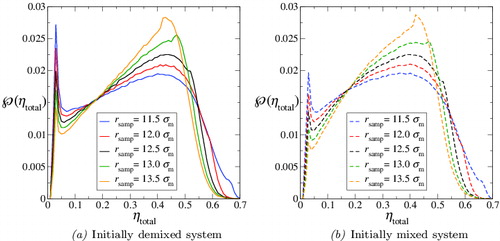
Figure A2. The sampling-sphere radius, r _samp, does not affect the comparison of the initially demixed (continuous curves) and initially mixed (dashed curves) simulations, in terms of the calculated probability distributions of the total packing fraction, $\mathcal{P}\left({\eta }_{\mathrm{total}}\right)$, which is here reaffirmed to be essentially the same for the two systems, irrespective of the value of r _samp. The conclusion that both simulations have converged to configurations with the same distribution of density is thereby shown not to rely on the chosen value of r _samp.

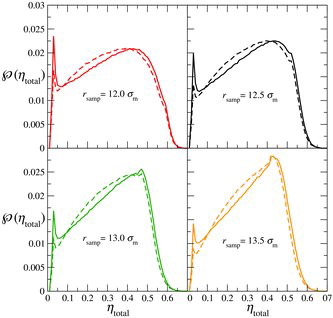
When the sampling radius, r _samp, is small the low-density peak in the probability distribution of the packing fraction, $\mathcal{P}\left({\eta }_{\mathrm{total}}\right)$, corresponding to the polymer-rich phase, is very sharp and well defined; although the peak broadens very slightly as r _samp is increased, it remains fairly sharp and well defined. Conversely, when r _samp is small, the peak in $\mathcal{P}\left({\eta }_{\mathrm{total}}\right)$ at higher density, corresponding to the colloid-rich phase, is broad and relatively flat. As r _samp is increased, the sampling of this phase improves and one observes the peak becoming much sharper. The value of the packing fraction at the maximum in this peak is essentially insensitive to r _samp, although at small r _samp there is a slight disagreement in this value between the initially demixed and initially mixed simulations, as can be seen in Figure A2; this disagreement disappears as r _samp is increased. A compromise value of r _samp = 12.5σ_m is chosen in our current work.

Appendix B. Scaling argument for range of depletion interaction

Even though the chains as a whole are not swollen, we picture a length scale (the blob size) such that within a blob a chain is locally swollen. Accordingly, at length scales shorter than the blob size, the scaling of segment separations, r, with the number of (separating) segments, n, is r ∼ n ^3/5, whereas at longer length scales, the scaling is r ∼ n ^1/2. The packing fraction at the crossover scales according to η_cross ∼ (n _bσ_m ³)/(n _b ^9/5σ_m ³) ≈ n _b ^{− 4/5}, where n _b is the number of segments per blob. Thereby n _cross ∼ η^−5/4; $\eta =0.075⇝n_{\mathrm{cross}}\approx 26$ segments. ξ then corresponds to the ‘radius of gyration’ of a chain of 26 segments. This can be estimated using data from reference [105] pertaining to the dimensions of tangent HS chains: $ln(\sqrt{6}\xi /{\sigma }_{\mathrm{m}})\approx (3/5)ln\left(26\right)+0.15⇝\xi \approx 3.3{\sigma }_{\mathrm{m}}$. Given that the chains under consideration are so short, this scaling argument probably leadsto a slight underestimate and hence the estimate in the main text: ξ ≈ 3σ_m to 4σ_m.

References

- H.N.W. Lekkerkerker and R. Tuinier , Colloids and the Depletion Interaction, Lecture Notes in Physics , Vol. 833 (Springer, Heidelberg, 2011).
- F.K.R. Li-In-On , B. Vincent , and F.A. Waite , ACS Symp. Ser. 9 , 165 (1975).
- F.L. Calderon , J. Bibette , and J. Bais , Europhys. Lett. 23 , 653 (1993).
- P.N. Pusey , A.D. Pirie , and W.C.K. Poon , Phys. A 201 , 322 (1993).
- P.N. Pusey , W.C.K. Poon , S.M. Ilett , and P. Bartlett , J. Phys. 6 , A29 (1994).
- W.C.K. Poon , A.D. Pirie , and P.N. Pusey , Faraday Discuss. 101 , 65 (1995).
- A.D. Dinsmore , A.D. Yodh , and D.J. Pine , Phys. Rev. E 52 , 4045 (1995).
- N.A.M. Verhaegh , J.S. van Duijneveldt , J.K.G. Dhont , and H.N.W. Lekkerkerker , Phys. A 230 , 409 (1996).
- I. Bodnar and W.D. Oosterbaan , J. Chem. Phys. 106 , 7777 (1997).
- R. Verma , J.C. Crocker , T.C. Lubensky , and A.G. Yodh , Phys. Rev. Lett. 81 , 4004 (1998).
- A. Moussaïd , W.C.K. Poon , P.N. Pusey , and M.F. Soliva , Phys. Rev. Lett. 82 , 225 (1999).
- F. Renth , W.C.K. Poon , and R.M.L. Evans , Phys. Rev. E 64 , 031402 (2001).
- S. Ramakrishnan , M. Fuchs , K.S. Schweizer , and C.F. Zukoski , J. Chem. Phys. 116 , 2201 (2002).
- H. de Hek and A. Vrij , J. Colloid Interface Sci. 84 , 409 (1981).
- C. Pathmamanoharan , H. de Hek , and A. Vrij , Colloid Polymer Sci. 259 , 769 (1981).
- A.P. Gast , C.K. Hall , and W.B. Russel , J. Colloid Interface Sci. 96 , 251 (1983).
- P.R. Sperry , J. Colloid Interface Sci. 99 , 97 (1984).
- A.P. Gast , W.B. Russel , and C.K. Hall , J. Colloid Interface Sci. 109 , 161 (1986).
- B. Vincent , J. Edwards , S. Emmett , and R. Croot , Colloids Surf. 31 , 267 (1988).
- P.D. Patel and W.B. Russel , J. Colloid Interface Sci. 131 , 192 (1989).
- C. Smits , J.S. van Duijneveldt , J.K.G. Dhont , H.N.W. Lekkerkerker , and W.M. Briels , Phase Transit. 21 , 157 (1990).
- C. Smits , B. van der Most , J.K.G. Dhont , H.N.W. Lekkerkerker , and W.M. Briels , Adv. Colloid Interface Sci. 42 , 33 (1992).
- W.C.K. Poon , J. Phys.: Condens. Matter 14 , R859 (2002).
- D.G.A.L. Aarts and H.N.W. Lekkerkerker , J. Phys.: Condens. Matter 16 , S4231 (2004).
- H.N.W. Lekkerkerker , V. de Villeneuve , J. de Folter , M. Schmidt , Y. Hennequin , D. Bonn , J. Indekeu , and D.G.A.L. Aarts , Eur. Phys. J. A 64 , 341 (2008).
- Y. Hennequin , D.G.A.L. Aarts , J.O. Indekeu , H.N.W. Lekkerkerker , and D. Bonn , Phys. Rev. Lett. 100 , 178305 (2008).
- E.A.G. Jamie , R.P.A. Dullens , and D.G.A.L. Aarts , J. Chem. Phys. 137 , 204902 (2012).
- S. Asakura and F. Oosawa , J. Chem. Phys. 22 , 1255 (1954).
- S. Asakura and F. Oosawa , J. Polym. Sci. 33 , 183 (1958).
- A. Vrij , Pure Appl. Chem. 48 , 471 (1976).
- W.C.K. Poon and P.N. Pusey , in Observation, Prediction and Simulation of Phase Transitions in Complex Fluids, NATO Science Series C: Mathematical and Physical Science , Vol. 460, edited by M. Baus , L.F. Rull , and J. Ryckaert (Kluwer Academic, Dordrecht, 1995).
- C.N. Likos , Phys. Rep. 348 , 267 (2001).
- K.J. Mutch , J.S. van Duijneveldt , and J. Eastoe , Soft Matter 3 , 155 (2007).
- G.J. Fleer and R. Tuinier , Adv. Colloid Interface Sci. 143 , 1 (2008).
- K. Binder , P. Virnau , and A. Statt , J. Chem. Phys. 141 , 140901 (2014).
- R. Dickman and A. Yethiraj , J. Chem. Phys. 100 , 4683 (1994).
- R. Tuinier , G.A. Vliegenthart , and H.N.W. Lekkerkerker , J. Chem. Phys. 113 , 10768 (2000).
- A.A. Louis , P.G. Bolhuis , E.J. Meijer , and J.-P. Hansen , J. Chem. Phys. 117 , 1893 (2002).
- M. Doxastakis , Y.L. Chen , O. Guzman , and J.J. de Pablo , J. Chem. Phys. 120 , 9335 (2004).
- A. Striolo , C.M. Colina , K.E. Gubbins , N. Elvassore , and L. Lue , Mol. Simul. 30 , 437 (2004).
- M. Doxastakis , Y.L. Chen , and J.J. de Pablo , J. Chem. Phys. 123 , 034901 (2005).
- X. Chen , J. Cai , H. Liu , and Y. Hu , Mol. Simul. 32 , 877 (2006).
- A. Bymaster , S. Jain , and W.G. Chapman , J. Chem. Phys. 128 , 164910 (2008).
- R.W. Zwanzig , J. Chem. Phys. 22 , 1420 (1954).
- J.A. Barker and D. Henderson , J. Chem. Phys. 47 , 2856 (1967).
- H.N.W. Lekkerkerker , W.C.K. Poon , P.N. Pusey , A. Stroobants , and P.B. Warren , Europhys. Lett. 20 , 559 (1992).
- K.G. Honnell and C.K. Hall , J. Chem. Phys. 90 , 1841 (1989).
- R.P. Sear and D. Frenkel , Phys. Rev. E 55 , 1677 (1997).
- P.B. Warren , Langmuir 13 , 4588 (1997).
- D.G.A.L. Aarts , R. Tuinier , and H.N.W. Lekkerkerker , J. Phys.: Condens. Matter 14 , 7551 (2002).
- M. Fuchs and K.S. Schweizer , J. Phys.: Condens. Matter 14 , R239 (2002).
- A. Moncho-Jordá , B. Rotenberg , and A.A. Louis , J. Chem. Phys. 119 , 12667 (2003).
- P. Paricaud , S. Varga , and G. Jackson , J. Chem. Phys. 118 , 8525 (2003).
- P. Paricaud , S. Varga , P.T. Cummings , and G. Jackson , Chem. Phys. Lett. 398 , 489 (2004).
- P. Bryk , J. Chem. Phys. 122 , 064902 (2005).
- G.J. Fleer and R. Tuinier , Phys. Rev. E 76 , 041802 (2007).
- J.O. Indekeu , D.G.A.L. Aarts , H.N.W. Lekkerkerker , Y. Hennequin , and D. Bonn , Phys. Rev. E 81 , 041604 (2010).
- S. Jain , P. Jog , J. Weinhold , R. Srivastava , and W.G. Chapman , J. Chem. Phys. 128 , 154910 (2008).
- M.S. Wertheim , J. Chem. Phys. 87 , 7323 (1987).
- W.G. Chapman , G. Jackson , and K.E. Gubbins , Mol. Phys. 65 , 1057 (1988).
- J. Forsman and C.E. Woodward , Phys. Rev. E 73 , 051803 (2006).
- T. Zykova-Timan , J. Horbach , and K. Binder , J. Chem. Phys. 133 , 014705 (2010).
- E.J. Meijer and D. Frenkel , Phys. Rev. Lett. 67 , 1110 (1991).
- E.J. Meijer and D. Frenkel , J. Chem. Phys. 100 , 6873 (1994).
- P.G. Bolhuis and D. Frenkel , J. Chem. Phys. 101 , 9869 (1994).
- E.J. Meijer and D. Frenkel , Phys. A 213 , 130 (1995).
- M. Dijkstra , J.M. Brader , and R. Evans , J. Phys.: Condens. Matter 11 , 10079 (1999).
- A.A. Louis , P.G. Bolhuis , E.J. Meijer , and J.-P. Hansen , J. Chem. Phys. 116 , 10547 (2002).
- B. Rotenberg , J. Dzubiella , J.-P. Hansen , and A.A. Louis , Mol. Phys. 102 , 1 (2004).
- R.L.C. Vink , A. Jusufi , J. Dzubiella , and C.N. Likos , Phys. Rev. E 72 , 030401 (2005).
- N.A. Mahynski , T. Lafitte , and A.Z. Panagiotopoulos , Phys. Rev. E 85 , 051402 (2012).
- D. Meng , S.K. Kumar , S.F. Cheng , and G.S. Grest , Soft Matter 9 , 5417 (2013).
- A.A. Louis , P.G. Bolhuis , J.-P. Hansen , and E.J. Meijer , Phys. Rev. Lett. 85 , 2522 (2000).
- P.G. Bolhuis , A.A. Louis , J.-P. Hansen , and E.J. Meijer , J. Chem. Phys. 114 , 4296 (2001).
- P.G. Bolhuis , A.A. Louis , and J.-P. Hansen , Phys. Rev. E 64 , 021801 (2001).
- P.G. Bolhuis and A.A. Louis , Macromolecules 35 , 1860 (2002).
- P.G. Bolhuis , A.A. Louis , and J.-P. Hansen , Phys. Rev. Lett. 89 , 128302 (2002).
- R.L.C. Vink and J. Horbach , J. Chem. Phys. 121 , 3253 (2004).
- R.L.C. Vink , J. Horbach , and K. Binder , J. Chem. Phys. 122 , 134905 (2005).
- R.L.C. Vink , J. Horbach , and K. Binder , Phys. Rev. E 71 , 011401 (2005).
- T.W. Rosch and J.R. Errington , J. Chem. Phys. 129 , 164907 (2008).
- C. Chou , T. Vo , A. Panagiotopoulos , and M. Robert , Phys. A 369 , 275 (2006).
- F.W. Starr , J.F. Douglas , and S.C. Glotzer , J. Chem. Phys. 119 , 1777 (2003).
- F. Lo Verso , L. Yelash , S.A. Egorov , and K. Binder , J. Chem. Phys. 135 , 214902 (2011).
- N.A. Mahynski , B. Irick , and A.Z. Panagiotopoulos , Phys. Rev. E 87 , 022309 (2013).
- N.A. Mahynski , A.Z. Panagiotopoulos , D. Meng , and S.K. Kumar , Nat. Commun. 5 , 4472 (2014).
- N.A. Mahynski , S.K. Kumar , and A.Z. Panagiotopoulos , Soft Matter 11 , 280 (2015).
- J.D. Weeks , D. Chandler , and H.C. Andersen , J. Chem. Phys. 54 , 5237 (1971).
- M. Surve , V. Pryamitsyn , and V. Ganesan , J. Chem. Phys. 122 , 154901 (2005).
- A. Pelissetto and J.-P. Hansen , Macromolecules 39 , 9571 (2006).
- W.K. Lim and A.R. Denton , J. Chem. Phys. 141 , 114909 (2014).
- A.A. Shvets and A.N. Semenov , J. Chem. Phys. 139 , 054905 (2013).
- R. Tuinier , D.G.A.L. Aarts , H.H. Wensink , and H.N.W. Lekkerkerker , Phys. Chem. Chem. Phys. 5 , 3707 (2003).
- L. Feng , B. Laderman , S. Sacanna , and P. Chaikin , Nat. Mater. 14, 61 (2015).
- T. Lafitte , A. Apostolakou , C. Avendaño , A. Galindo , C.S. Adjiman , E.A. Müller , and G. Jackson , J. Chem. Phys. 139 , 154504 (2013).
- V. Papaioannou , T. Lafitte , C. Avendaño , C.S. Adjiman , G. Jackson , E.A. Müller , and A. Galindo , J. Chem. Phys. 14 , 054107 (2014).
- C. Avendaño , T. Lafitte , A. Galindo , C.S. Adjiman , G. Jackson , and E.A. Müller , J. Phys. Chem. B 115 , 11154 (2011).
- C. Avendaño , T. Lafitte , C.S. Adjiman , A. Galindo , E.A. Müller , and G. Jackson , J. Phys. Chem. B 117 , 2717 (2013).
- T. Lafitte , C. Avendaño , V. Papaioannou , A. Galindo , C.S. Adjiman , G. Jackson , and E.A. Müller , Mol. Phys. 110 , 1189 (2012).
- O. Lobanova , C. Avendaño , T. Lafitte , E.A. Müller , and G. Jackson , Mol. Phys. 113, 1228 (2015).
- E.A. Müller and G. Jackson , Ann. Rev. Chem. Biomol. Eng. 5 , 405 (2014).
- C. Herdes , E.E. Santiso , C. James , J. Eastoe , and E.A. Müller , J. Colloid Interface Sci. 445 , 16 (2015).
- P.E. Theodorakis , E.A. Müller , R.V. Craster , and O.K. Matar , Langmuir 31 , 2304 (2015).
- S. Rahman , O. Lobanova , C. Correia-Braga , V. Raptis , E.A. M üller, G. Jackson , and A. Galindo , Submitted (2015).
- A.J. Haslam , G. Jackson , and T.C.B. McLeish , J. Chem. Phys. 111 , 416 (1999).
- J.F. Jover , A.J. Haslam , A. Galindo , G. Jackson , and E.A. Müller , J. Chem. Phys. 137 , 144505 (2012).
- T. Boublík , J. Chem. Phys. 53 , 471 (1970).
- G.A. Mansoori , N.F. Carnahan , K.E. Starling , and T.W. Leland , J. Chem. Phys. 54 , 1523 (1971).
- G. Jackson , J.S. Rowlinson , and F. Van Swol , J. Phys. Chem. 91 , 4907 (1987).
- E.A. Müller and K.E. Gubbins , Mol. Phys. 80 , 957 (1993).
- T. Boublík , Mol. Phys. 68 , 191 (1989).
- T. Boublík , C. Vega , and M. Diaz-Peña , J. Chem. Phys. 93 , 730 (1990).
- W. Smith and T.R. Forester , J. Mol. Graphics 14 , 136 (1996).
- D. Beeman , J. Comput. Phys. 20 , 130 (1976).
- J.-P. Ryckaert , G. Ciccotti , and H.J.C. Berendsen , J. Comput. Phys. 23 , 327 (1977).
- J.M. Brader , R. Evans , and M. Schmidt , Mol. Phys. 101 , 3349 (2003).
- L.D. Gelb and E.A. Müller , Fluid Phase Equilib. 203 , 1 (2002).
- F.J. Martínez-Veracoechea and E.A. Müller , Mol. Simul. 31 , 33 (2005).
- W.G. Hoover and F.H. Ree , J. Chem. Phys. 49 , 3609 (1968).
- K. Binder , Phys. Rev. A 25 , 1699 (1982).
- J.J. Potoff and A.Z. Panagiotopoulos , J. Chem. Phys. 112 , 6411 (2000).
- G.J. Gloor , G. Jackson , F.J. Blas , and E. de Miguel , J. Chem. Phys. 123 , 134703 (2005).
- D.G.A.L. Aarts , M. Schmidt , and H.N.W. Lekkerkerker , Science 304 , 847 (2004).
- D. Frenkel , Phys. A 263 , 26 (1999).
- X.-Z. Cao , H. Merlitz , C.-X. Wu , and J.-U. Sommer , Phys. Rev. E 84 , 041802 (2011).
- J.F. Joanny , L. Leibler , and P.G. de Gennes , J. Polym. Sci. B 17 , 1073 (1979).
- X.-Z. Cao , H. Merlitz , C.-X. Wu , and J.-U. Sommer , Soft Matter 9 , 5916 (2013).
- A.J. Haslam , G. Jackson , and T.C.B. McLeish , Macromolecules 32 , 7289 (1999).
- D. Frenkel and B. Smit , Understanding Molecular Simulation from Algorithms to Applications , Computational Science Series , 2nd ed. (Academic Press, San Diego, CA, 2002).
- L.S. Ornstein and F. Zernike , Proc. Akad. Sci. (Amsterdam) 17 , 793 (1914), reproduced in H. Frisch and J.L. Lebowitz , The Equilibrium Theory of Classical Fluids (Benjamin, New York, 1964).
- J.M.J. van Leeuwen , J. Groeneveld , and J. de Boer , Physica 25 , 792 (1959).
- B. Lu and A.R. Denton , J. Phys. 23 , 285102 (2011).