Atomic shell structure determined by the curvature of the electron position uncertainty

abstract

The electron density logarithm is closely connected to the Shannon information entropy characterising the spread of the electron density. It can be seen as the uncertainty to predict the position of an electron. The position uncertainty curvature, defined as the negative of the Laplacian of the electron density logarithm, describes regions of space where the uncertainty of the electron position is higher, respectively lower, than the average in the surrounding. The atomic shells can be located in regions of high-position uncertainty curvature, thus resolving the atomic shell structure of the atoms Li to Xe. The shell boundaries are given as minima of the uncertainty curvature. This indicator, based alone on the electron density, is suitable to describe the bonding situation in molecules and solids.

GRAPHICAL ABSTRACT

Keywords:

• Atomic shell structure
• information entropy
• position uncertainty

1. Introduction

The spherically averaged electron density $\rho \left(\mathit{r}\right)$ of an atom displays a maximum at the atomic position followed by monotonically exponential decay [1–5]. The idea of atomic shells successively filled up by electrons, as anticipated from the Periodic Table of elements, is not directly reflected by this simple distribution. To accomplish this, specific functions derived from the electron density or even functions based on the orbital representation of wave function are needed. The analysis of such functions revealed, at least partially, the atomic shell structure [2,4,6–22]. However, only few functionals were able not only to resolve the atomic shell structure, but also to yield reasonable electron populations for the shell occupations, for instance the average local electrostatic potential [18], the electron localisation function (ELF) [14,17], as well as ELF modified by the incorporation of the electrostatic potential [19], respectively, the electron localisability indicator (ELI) [23–25] and the one-electron potential (OEP) [20]. The electron localisability indicator variant ELI-D [26] yields at the Hartree–Fock (HF) level in principle the same topology as ELF, but in contrast to ELF is defined also at correlated level of theory [26,27].

The piecewise exponential decay of the electron density $\rho \left(\mathit{r}\right)$ of an atom was investigated by Wang and Parr [4] who showed that for the ground state of atoms, the function $log\rho \left(\mathit{r}\right)$ reflects shell structure by a significant change of the $log\rho \left(\mathit{r}\right)$ slope. This circumstance was used later for the quantity $-\left|\nabla \rho \right(\mathit{r}\left)\right|/\rho \left(\mathit{r}\right)$ displaying separate plateaus for each atomic shell [16]. For the quantitative evaluation of the atomic shells, suitable separators were needed to determine the shell boundaries of $-\left|\nabla \rho \right(\mathit{r}\left)\right|/\rho \left(\mathit{r}\right)$. Bohórquez and Boyd, after connecting $-\nabla \rho \left(\mathit{r}\right)/\rho \left(\mathit{r}\right)$ with the quantum spread, used the radial inflection points as the shell delimiters [21]. Of course, such definition based on spherical symmetry is in principle applicable only to shells of free atoms. In the present study, a function derived from the electron density logarithm was used to visualise and analyse the shell structure of atoms. The function can easily be applied also to the analysis of bonding situation in molecules and solids.

2. Theory

For the quantity X of n discrete values x_i measured with the respective probabilities p_i the expression: (1) $$S_p=-\sum _i^n{p}_{i}log{p}_i$$(1) is the Boltzmann–Shannon information entropy of the measurement [28]. The information entropy describes the uncertainty to obtain one (further not specified) discrete value of the quantity X. If specific event has the probability p_k = 1 and the remaining ones equal zero, then the information entropy S_p = 0. Of course, in this case, the result of the measurement will be certainly x_k. On the other hand, if all n values occur with the same probability p_i = 1/n the uncertainty about the outcome of the measurement reaches its maximum and the information entropy S_p = log n. The information entropy as given by Equation (1(1) $$S_p=-\sum _i^n{p}_{i}log{p}_i$$(1) ) can also be seen as the average value of the quantity Y of n discrete values y_i = −log p_i occurring with the probabilities p_i. Each single value −log p_i can be regarded as the uncertainty to obtain the value x_i for the quantity X.

The electron density $\rho \left(\mathit{r}\right)$ is connected with the probability (multiplied by the number of electrons in the system) of finding the coordinates of an electron between $\mathit{r}$ and $d\mathit{r}$, with the remaining electrons distributed anywhere in the space. Let us take for the measured quantity the determination of the position $\mathit{r}$ of an electron. The information entropy S_ρ for this measurements, describing the spread of the electron density, is given by: (2) $$S_{\rho }=-\int \rho \left(\mathit{r}\right)log\rho \left(\mathit{r}\right)\mathrm{d}\mathit{r}.$$(2) In accordance with the discrete case, the function $-log\rho \left(\mathit{r}\right)$ can be interpreted as the uncertainty in the prediction of the electron position and the information entropy S_ρ as the mean value of this uncertainty [29]. Often the terms local Shannon information for $s\left(\mathit{r}\right)=-\rho \left(\mathit{r}\right)log\rho \left(\mathit{r}\right)$ as well as Shannon information density per particle for the function $-log\rho \left(\mathit{r}\right)$ are used [30]. Shannon entropy was also connected with the correlation strength [31] as well as utilised in the orbital-free density-functional theory (DFT) [32]. The combined Shannon entropies in position and momentum space are involved in the derivation of the Heisenberg uncertainty relation [33].

The investigation of Wang and Parr [4] and Kohout et al. [16] corroborated the idea that the electron position uncertainty $-log\rho \left(\mathit{r}\right)$ as well as its gradient $-\mathit{}\nabla \rho \left(r\right)/\rho \left(r\right)$, also termed the local wave-vector, is able to detect the shell structure of atoms. However, as Wang and Parr stated ‘... the transitions from one exponential to the next occur over certain intervals and cannot be associated with single points.’ Some years later, Bohórquez and Boyd connected $-\mathit{}\nabla \rho \left(r\right)/\rho \left(r\right)$ with the so-called quantum spread $\mathit{}\tilde{\mathbf{P}}$, which is a part of the local representation of the momentum operator [21]: (3) $$\mathit{}\tilde{\mathbf{P}}\left(\mathit{r}\right)=-\frac{\hslash }{2}\frac{\mathit{}\nabla \rho \left(\mathit{r}\right)}{\rho \left(\mathit{r}\right)}.$$(3) Analysing the representation of the atomic shell structure with the magnitude of the quantum spread $\tilde{P}$, the above authors defined the radial inflection points ${\partial }^2\tilde{P}/\partial r^2=0$ located after each local maximum as the shell boundaries. The application of this procedure for some closed shell atoms yielded shell populations close to the one of ELF, with somewhat lower populations of the first shell when compared to the ELF results (which overestimate the first shell population) [21]. This approach could easily be applied also to atoms with spherically averaged electron density. However, it would be more complex to employ such definition of the shell boundaries for molecules due to the los of the sphericity.

This obstacle can be simply circumvented by the utilisation of the Laplacian of the electron position uncertainty, instead of the radial curvature. Let us define the position uncertainty curvature (PUC): (4) $$\mathrm{PUC}=-{\nabla }^{2}log\rho \left(\mathit{r}\right)={\left[\frac{\mathit{}\nabla \rho \left(\mathit{r}\right)}{\rho \left(\mathit{r}\right)}\right]}^2-\frac{{\nabla }^2\rho \left(\mathit{r}\right)}{\rho \left(\mathit{r}\right)}.$$(4) The PUC is given by two term – the scaled density gradient and the scaled density Laplacian, respectively – in ratio 1:1. Interestingly, there is another density function also composed of these two terms, namely the OEP defined by $1/2\left({\nabla }^2\sqrt{\rho }\right)/\sqrt{\rho }$ [12,34]. For OEP, the corresponding ratio of the two terms is 1:2. The OEP was used to visualise the chemical bonding [12] and it nicely resolves the atomic shell structure [20].

In case of spherical symmetry, the ∇² operator is replaced by ∂²/∂r² + (2/r)∂/∂r, i.e. the second right-side term of Equation (4(4) $$\mathrm{PUC}=-{\nabla }^{2}log\rho \left(\mathit{r}\right)={\left[\frac{\mathit{}\nabla \rho \left(\mathit{r}\right)}{\rho \left(\mathit{r}\right)}\right]}^2-\frac{{\nabla }^2\rho \left(\mathit{r}\right)}{\rho \left(\mathit{r}\right)}.$$(4) ) will be split into two contributions. For large distances from the nucleus ρ(r) ≈ kr^βe^−αr (with k, α > 0 and β ≤ 0) [35]. Applying this to Equation (4(4) $$\mathrm{PUC}=-{\nabla }^{2}log\rho \left(\mathit{r}\right)={\left[\frac{\mathit{}\nabla \rho \left(\mathit{r}\right)}{\rho \left(\mathit{r}\right)}\right]}^2-\frac{{\nabla }^2\rho \left(\mathit{r}\right)}{\rho \left(\mathit{r}\right)}.$$(4) ) yields 2α/r − β/r², i.e. the PUC asymptotically approaches zero from above for infinite distance r. At the origin ,∇²ρ(r) is negative infinite, whereas the first term on the right hand side of Equation (4(4) $$\mathrm{PUC}=-{\nabla }^{2}log\rho \left(\mathit{r}\right)={\left[\frac{\mathit{}\nabla \rho \left(\mathit{r}\right)}{\rho \left(\mathit{r}\right)}\right]}^2-\frac{{\nabla }^2\rho \left(\mathit{r}\right)}{\rho \left(\mathit{r}\right)}.$$(4) ) approaches a constant (see for instance Ref. [10]). Hence, a positive infinite PUC is found at the atomic origin.

A positive curvature is found at such points, where the position uncertainty is lower than the average value in the closest neighbourhood. The uncertainty in the localisation of an electron (compared to the average value in the closest neighbourhood) decreases, i.e. the electron density is less spread, with increasing value of PUC. Thus, it is an appealing idea to assign the (positive) peaks in a $-{\nabla }^{2}log\rho \left(\mathit{r}\right)$ vs. radius diagram to the atomic shells and the positions of the minima between the peaks to the shell radii. This definition of shell radii based on PUC is reasonable also from another point of view. Namely, because for the second row atoms, two shells are expected (and two PUC maxima are indeed found, cf. Figure 1(a) for the Be atom). Whereas the first shell has a finite radius (correspondingly, there is a negative PUC minimum), the second one extends to infinity. In contrast, choosing the zeros of PUC as the shell delimiters would result in two finite shell radii (otherwise one of the odd or even zeros had to be chosen), cf. Figure 1(a). Because PUC is defined independently of the symmetry of the systems, it can be easily applied to molecules and crystals.

Figure 1. Atomic shells represented by PUC using the wave functions of Clementi and Roetti. (a) Be atom. (b) Ag atom. The spurious minimum at 4.43 bohr within the 5th shell is marked by the arrow.

3. Results and discussion

Using the wave functions of Clementi and Roetti [36] for the atoms Li to Xe, the spherically averaged electron densities ρ(r) as well as the PUC = −∇²log ρ were calculated with the DGrid program [37]. The minima of PUC were detected and assigned to the atomic shell radii. The electron density within the radial shells were integrated yielding the corresponding shell populations. The results are compiled in Table 1.

Table 1. The shell radii and electron populations given by the minima of −∇²log (ρ).

Atom	q^K	r^K	q^L	r^L	q^M	r^M	q^N	r^N	q^O
^3Li (^2S)	2.0	1.605	1.0	–	–	–	–	–	–
^4Be (^1S)	2.0	1.018	2.0	–	–	–	–	–	–
^5B (^2P)	2.0	0.746	3.0	–	–	–	–	–	–
^6C (^3P)	2.1	0.582	3.9	–	–	–	–	–	–
^7N (^4S)	2.1	0.475	4.9	–	–	–	–	–	–
^8O (^3P)	2.1	0.399	5.9	–	–	–	–	–	–
^9F (^2P)	2.1	0.343	6.9	–	–	–	–	–	–
^10Ne (^1S)	2.2	0.300	7.8	–	–	–	–	–	–
^11Na (^2S)	2.2	0.265	7.9	2.257	0.9	–	–	–	–
^12Mg (^1S)	2.2	0.238	7.9	1.687	1.9	–	–	–	–
^13Al (^2P)	2.2	0.215	7.9	1.394	2.9	–	–	–	–
^14Si (^3P)	2.2	0.197	7.8	1.185	3.9	–	–	–	–
^15P (^4S)	2.2	0.181	7.8	1.029	4.9	–	–	–	–
^16S (^3P)	2.2	0.168	7.8	0.910	5.9	–	–	–	–
^17Cl (^2P)	2.2	0.156	7.8	0.813	6.9	–	–	–	–
^18Ar (^1S)	2.2	0.146	7.8	0.735	7.9	–	–	–	–
^19K (^2S)	2.2	0.137	7.8	0.670	8.0	3.240	0.9	–	–
^20Ca (^1S)	2.2	0.129	7.8	0.615	8.0	2.536	1.9	–	–
^21Sc (^2D)	2.2	0.122	7.8	0.571	8.8	2.372	2.1	–	–
^22Ti (^3F)	2.2	0.116	7.9	0.532	9.8	2.290	2.1	–	–
^23V (^4F)	2.3	0.110	7.9	0.498	10.7	2.210	2.1	–	–
^24Cr (^7S)	2.3	0.105	8.0	0.469	12.4	2.412	1.3	–	–
^25Mn (^6S)	2.3	0.100	8.0	0.442	12.6	2.104	2.1	–	–
^26Fe (^5D)	2.3	0.096	8.1	0.418	13.5	2.043	2.1	–	–
^27Co (^4F)	2.3	0.092	8.1	0.396	14.5	1.995	2.1	–	–
^28Ni (^3F)	2.3	0.088	8.2	0.376	15.5	1.955	2.1	–	–
^29Cu (^2S)	2.3	0.085	8.2	0.359	17.6	2.557	0.9	–	–
^30Zn (^1S)	2.3	0.082	8.3	0.342	17.4	1.888	2.1	–	–
^31Ga (^2P)	2.3	0.079	8.3	0.327	17.4	1.644	3.0	–	–
^32Ge (^3P)	2.3	0.076	8.3	0.313	17.3	1.454	4.1	–	–
^33As (^4S)	2.3	0.074	8.4	0.299	17.3	1.311	5.1	–	–
^34Se (^3P)	2.3	0.071	8.4	0.287	17.3	1.202	6.0	–	–
^35Br (^2P)	2.3	0.069	8.4	0.276	17.2	1.103	7.1	–	–
^36Kr (^1S)	2.3	0.067	8.4	0.266	17.2	1.023	8.1	–	–
^37Rb (^2S)	2.3	0.065	8.5	0.256	17.1	0.955	8.2	3.691	0.9
^38Sr (^1S)	2.3	0.063	8.5	0.247	17.1	0.896	8.2	2.940	1.9
^39Y (^1S)	2.3	0.061	8.5	0.239	17.1	0.850	8.9	2.728	2.2
^40Zr (^1S)	2.3	0.060	8.6	0.231	17.1	0.810	10.3	2.797	1.7
^41Nb (^1S)	2.3	0.058	8.6	0.224	17.1	0.771	11.4	2.768	1.7
^42Mo (^1S)	2.3	0.057	8.6	0.217	17.1	0.739	12.6	2.880	1.4
^43Tc (^1S)	2.3	0.055	8.6	0.210	17.1	0.702	12.9	2.581	2.1
^44Ru (^1S)	2.3	0.054	8.6	0.204	17.1	0.674	16.0	–	–
^45Rh (^1S)	2.3	0.053	8.7	0.198	17.1	0.646	17.0	–	–
^46Pd (^1S)	2.3	0.051	8.7	0.193	17.1	0.621	17.2	2.760	0.7
^47Ag (^1S)	2.3	0.050	8.7	0.188	17.1	0.597	18.0	3.010	0.9^a
^48Cd (^1S)	2.3	0.049	8.8	0.183	17.1	0.576	18.2	2.528	1.7
^49In (^1S)	2.3	0.048	8.8	0.178	17.1	0.552	18.1	2.160	2.8
^50Sn (^1S)	2.3	0.047	8.8	0.174	17.0	0.533	18.0	1.901	3.9
^51Sb (^1S)	2.3	0.046	8.8	0.169	17.0	0.514	17.9	1.719	5.0
^52Te (^1S)	2.3	0.045	8.8	0.165	17.0	0.497	17.9	1.581	6.0
^53I (^1S)	2.3	0.044	8.8	0.161	17.0	0.481	17.8	1.467	7.1
^54Xe (^1S)	2.3	0.043	8.8	0.158	17.0	0.465	17.7	1.370	8.2

Note:q^K, electronic population in the K shell; r^K, radius of the K shell (in a.u.).

^aThe valence shell of Ag is split by shallow minimum at 4.43 bohr into two regions, populated by 0.6e and 0.3e, respectively.

The shell radii, and thus also the shell populations, are very close to the data obtained for ELF using the so-called ‘closed-shell’ formula [17] (at the single-determinantal level this applies also to ELI-D). The shell populations of the first three shells as given by PUC differ at most by 0.1 electrons from the data determined by the ELF. Correspondingly, this means that also for PUC the first shell is slightly over-populated by 2.3 electrons, starting already at the V atom. The same is true for the second shell occupied up to 8.8 electrons in case of Cd to Xe. In contrast, up to 1 electron is missing in the third shell (in case of full occupation according to the Periodic Table). In case of PUC, the shell occupations of the fourth shell are closer to 18 electrons (for full shell occupation) than are the corresponding shell populations determined for the ELF.

There are four exceptions where the valence shells are not properly resolved. In case of the Pd atom, the fifth shell is not occupied according to the Aufbau principle. However, PUC shows an unexpected minimum for the shell boundary with 0.7 electrons present in this spurious ‘valence’ shell. Indeed, this behaviour is similar to the one for atomic shells determined from the OEP, in which case even 2.3 electrons are found in such fifth shell for the Pd atom [20]. The another exception is the Ag atom for which the ‘ideal’ shell occupation [38] assumes 1 electron in the valence shell. Similarly, ELF delivers 1.1 electron for the fifth shell, whereas the OEP valence shell is over-populated by 2.8 electrons [20]. Although there are 0.9 electrons outside the fourth PUC shell for the Ag atom, cf. Table 1, the valence shell is split into two parts. As can be seen from Figure 1(b), there is a shallow PUC minimum at 4.43 bohr which formally splits the valence shell of Ag into a part populated by 0.6 electrons and an outer part populated by 0.3 electrons.

The two remaining exceptions concern a missing valence shell. For the atoms Ru and Rh, the Aufbau principle predicts valence shells occupied by 1 electron. The ELF resolves the valence shells for both atoms, with reasonable occupations of 1.3 and 1.2 electrons for Ru and Rh, respectively. Even the OEP shows separate valence shell for Ru and Rh, although heavily over-populated by almost 3 electrons. In contrast, there are no populations given in Table 1 for the fifth shell of Ru and Rh. The inspection of Figure 2 helps to clarify this issue. Whereas all four inner shells of Ru and Rh are well represented by PUC maxima, there is in both cases only a shoulder indirectly suggesting the presence of the valence shell. Not even the utilisation of a wave function from, for instance, a relativistic density functional calculation will amend this feature.

Figure 2. Atomic shells represented by PUC using the wave functions of Clementi and Roetti. The arrows mark the shoulder present instead of the 5th shell maximum. (a) Ru atom. (b) Rh atom.

Proper representation of the atomic shell structure is an essential prerequisite for plausible analysis of the bonding situation in molecules and solids. Then, the core regions which do not strongly participate on the bonding can be reasonably separated in the position space from the valence region that can be subsequently analysed in detail. As an example, the bonding of the cyclopropane C₃H₆ was analysed with PUC. The C₃H₆ was computed with the program GAMESS [39] at the HF level using the correlation consistent triplet zeta basis set CCT. The optimised HF distances amount to d(CC) = 2.828 bohr and d(CH) = 2.028 bohr, respectively. With the program DGrid, the output of GAMESS was converted into a wave function data file and the PUC distribution computed on an equidistant grid of 0.025 bohr mesh size.

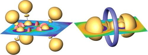
In Figure 3(a), the spherical isosurfaces of PUC = 4.25 marking the core regions of the carbon atoms can be observed. The corresponding core PUC basins enclose 2.09 electrons. This is a situation closely resembling the ELI-D results for the HF calculation of C₃H₆. The 4.25-localisation domains include the almost spherical isosurfaces around the hydrogen positions. Additionally, there are also isosurfaces located between the C and H isosurfaces along the C–H line. Each hydrogen PUC basin encloses 1.32 electrons, whereas the C–H basin is populated by 0.75 electrons. This is a situation very different from the one for ELI-D (respectively, ELF), which typically shows only a single hydrogen localisation domain with an ELI-D basin populated (in case of C₃H₆) by 2.03 electrons. A separate ELI-D domain between the C and H atoms is not present. Similarly, there are two localisation domains, displayed in Figure 3(a) as red coloured isosurfaces of PUC = 3.0, between the carbon atoms. In case of ELI-D, there is only single localisation domain (single attractor) representing the C–C bond. This behaviour can be easily explained by the inspection of the PUC and ELI-D topology for the free atoms. Whereas the positions of the minima (the atomic shell boundaries) are almost identical, the positions of the shell maxima for PUC (1.028 bohr) and ELI-D (1.488 bohr) are very different for the C atom. Taking as a first approximation for the C–C bond a simple overlap of the atomic PUC and ELI-D distributions shows that the PUC maxima are much closer to the nuclei than the C–C midpoint (1.414 bohr), whereas the ELI-D maxima are located slightly behind the C–C midpoint. This is a typical topological feature of PUC showing separate shell maxima and corresponding saddle point as the signature of bond. Interestingly, this allows in certain sense to define kind of bond polarity, because the bond is represented by two PUC basins related to separate participating atom. Of course, in case of the C–C bond, each of the C atoms yields the same contribution (0.88e) to the population of the bond (super)basin. Similarly, considering the combined hydrogen and CH PUC-basin (together populated by 2.07e) as a ‘split’ ELI-D hydrogen basin would yield 64% of the combined population to be located at the H atom and 36% attributed to the C atom. This seems to be far too polar for the C–H bond in the cyclopropane.

Figure 3. PUC localisation domains for the C₃H₆ and N₂ molecules. (a) HF calculation of C₃H₆ using the CCT basis. Red coloured: isosurfaces of PUC = 3.0. Yellow coloured: isosurfaces of PUC = 4.25. (b) HF calculation of N₂ using the CCT basis. Blue coloured: 1.77-localisation domain. Yellow coloured: isosurfaces of PUC=4.4. (c) CISD calculation of N₂ using the CCT basis. Yellow coloured: 4.4-localisation domains. (d) DFT calculation of N₂ using the TZP basis. Yellow coloured: 4.2-localisation domains.

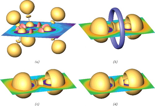
Figure 3(b) shows the PUC for the N₂ molecule computed with GAMESS at the HF level using the CCT basis set at the optimised distance of 2.017 bohr and evaluated on a grid of 0.025 bohr mesh size. Again, the core region can be nicely recognised by the two spherical 4.4-localisation domains. The correspond core basins are populated by 2.1 electrons. In the valence region, the two lone pair regions are visible by separate outwards pointing 4.4-localisation domains with the corresponding basins populated by 3.2 electrons. There is also a separate irreducible 4.4-localisation domain for the bond. Thus, for the HF wave function, there is only single PUC attractor at the bond line. The corresponding basin is populated by 2.9 electrons. Additionally, the blue coloured 1.77-localisation domain located around a ring attractor describes a second bond feature, with the basin populated by 0.4 electrons. Besides this ring attractor, the description of the nitrogen bond is similar to the one with ELI-D, also showing with 2.9e somewhat over-populated lone pair basins.

For the N₂ molecule, a configuration-interaction calculation was performed with single and double excitations (CISD) of 10 electrons (i.e. with inactive core electrons) into 58 orbitals using the CCT basis set (the optimised bond distance of 2.059 bohr was used). The PUC distribution shown in Figure 3(c) displays at first glance less features than the diagram for the HF calculation, because of the absence of the bonding ring localisation domain. Otherwise, the 4.4-localisation domains again mark the core regions and lone pair regions as well as the bonding region. The corresponding core, lone pair, and (combined) bond basins are populated by 2.1e, 3.8e, and 2.1e, respectively. This means that for the CISD wave function, the lone pair as represented by the PUC basin is even more over-populated than in case of the HF wave function. In contrast to the HF PUC topology, as already indicated above by the word ‘combined’, the bond basin for the CISD calculation is split into two basins, i.e. the 4.4-localisation domain in Figure 3(c) is reducible due to a shallow PUC saddle point at the bond midpoint.

For comparison, the DFT calculation of N₂ was performed with the ADF program [40–42] using the TZP basis set and the BLYP functional at the bond distance of 2.060 bohr. The PUC was computed on a grid of 0.025 bohr mesh size. Figure 3(d) with the 4.2-localisation domains shows the core and lone pair regions together with clearly separated localisation domains representing the bond. The populations of the corresponding basins is almost the same as the for the CISD calculation. The pronounced separation of the two bond PUC maxima results from changes in the electron density. The comparison between the electron density for the DFT and CISD calculation reveals slight decrease of the density in the bond and lone pair region accompanied by a density increase in the inter-shell regions. The density decrease around the bond midpoint changes the curvature of the electron density, thus, affecting the distribution of PUC.

4. Conclusion

The Shannon information entropy derived from the electron density describes the spread of the density. It can be seen as the mean value of the Shannon information density per particle $-log\rho \left(\mathit{r}\right)$, which is connected with the uncertainty in the prediction of the position of an electron. The position uncertainty can be inspected from the topological viewpoint by the analysis of its Laplacian. This defines the PUC = $-{\nabla }^{2}log\rho \left(\mathit{r}\right)$, that indicates whether the uncertainty is higher or lower than the average in the surrounding. PUC is able to resolve the atomic shell structure for almost all atoms from Li to Xe not only qualitatively but also to yield reasonable shell populations, similar to the one for ELI-D/ELF. The indicator PUC is applicable to molecules and crystals. It was demonstrated that localisation domains of PUC can be used as bonding descriptors representing core region, as well as lone pairs and bonds. Because the PUC atomic shell maxima are located closer to the corresponding nuclei, the bonds are usually characterised by two irreducible localisation domains and a PUC saddle point. The PUC is derived from the electron density and thus can be evaluated also from the experimental densities.

Disclosure statement

No potential conflict of interest was reported by the author.

References

- H. Weinstein, P. Politzer, and S. Srebenik, Theor. Chim. Acta 38, 159 (1975).
- A.M. Simas, R.P. Sagar, A.C.T. Ku, and V.H.J. Smith, Can. J. Phys. 66, 1923 (1988).
- G. Sperber, Int. J. Quantum Chem. 5, 189 (1971).
- W.P. Wang and R.G. Parr, Phys. Rew. A 16, 891 (1977).
- M. Hoffmann-Ostenhof and T. Hoffmann-Ostenhof, Phys. Rev. A 16, 1782 (1977).
- J.T. Waber and D.T. Cromer, J. Chem. Phys. 42, 4116 (1965).
- R.J. Boyd, Can. J. Phys. 56, 780 (1978).
- R.F.W. Bader, P.J. MacDougall, and C.D.H. Lau, J. Am. Chem. Soc. 106, 1594 (1984).
- R.F.W. Bader and H. Essén, J. Chem. Phys. 80, 1943 (1984).
- R.P. Sagar, A.C.T. Ku, V.H.J. Smith, and A.M. Simas, J. Chem. Phys. 88, 4367 (1988).
- Z. Shi and R.J. Boyd, J. Chem. Phys. 88, 4375 (1988).
- G. Hunter, Int. J. Quantum Chem. 29, 197 (1986).
- R.P. Sagar, A.C.T. Ku, and V.H.J. Smith, Can. J. Chem. 66, 1005 (1988).
- A.D. Becke and K.E. Edgecombe, J. Chem. Phys. 92, 5397 (1990).
- K.D. Sen, M. Slamet, and V. Sahni, Chem. Phys. Lett. 205, 313 (1993).
- M. Kohout, A. Savin, and H. Preuss, J. Chem. Phys. 95, 1928 (1991).
- M. Kohout and A. Savin, Int. J. Quantum Chem. 60, 875 (1996).
- K.D. Sen, T.V. Gayatri, and H. Toufar, J. Molec. Struct. (Theochem) 361, 1 (1996).
- P. Fuentealba, Int. J. Quantum Chem. 69, 559 (1998).
- M. Kohout, Int. J. Quantum Chem. 83, 324 (2001).
- H.J. Bohórquez and R.J. Boyd, Can. J. Phys. 56, 780 (1978).
- K. Wagner and M. Kohout, Theor. Chem. Acc. 128, 39 (2011).
- M. Kohout, Int. J. Quantum Chem. 97, 651 (2004).
- M. Kohout, Faraday Discuss. 135, 43 (2007).
- A. Martín Pendás, M. Kohout, M.A. Blanco, and E. Francisco, in Modern Charge-Density Analysis, edited by C. Gatti, and P. Macchi (Springer Dordrecht, Heidelberg, 2012).
- M. Kohout, K. Pernal, F.R. Wagner, and Y. Grin, Theor. Chem. Acc. 112, 453 (2004).
- M. Kohout, K. Pernal, F.R. Wagner, and Y. Grin, Theor. Chem. Acc. 113, 287 (2005).
- C.E. Shannon, Bell Syst. Tech. J. 27, 327 (1948).
- R.J. Yáñez, J.C. Angulo, and J.S. Dehesa, Int. J. Quantum Chem. 56, 489 (1995).
- A. Nagy and S. Liu, Phys. Lett. A 372, 1654 (2008).
- A.D. Gottlieb and N.J. Mauser, Phys. Rev. Lett. 95, 123003 (2005).
- A. Nagy, Int. J. Quantum Chem. 115, 1392 (2015).
- I. Białynicki-Birula and J. Mycielski, Commun. Math. Phys 44, 129 (1975).
- E.N. Lassettre, J. Chem. Phys. 83, 1709 (1985).
- M. Levy, J.P. Perdew, and V. Sahni, Phys. Rev. A 30, 2745 (1984).
- E. Clementi and C. Roetti, At. Data. Nucl. Data Tables 14, 218 (1974).
- M. Kohout, DGrid 5.0 Radebeul 2015.
- H. Schmider, R.P. Sagar, and V.H.J. Smith, Can. J. Chem. Phys. 70, 506 (1992).
- M.W. Schmidt, K.K. Baldridge, J.A. Boatz, S.T. Elbert, M.S. Gordon, J.H. Jensen, S. Koseki, N. Matsunaga, S. Koseki, N. Matsunaga, K.A. Nguyen, S.J. Su, T.L. Windus, M. Dupuis, and J.A. Montgomery, J. Comput. Chem. 14, 1347 (1993), GAMESS 2013.
- ADF2013, SCM, Theoretical Chemistry (Vrije Universiteit, Amsterdam). <http://www.scm.com>.
- G. te Velde, F.M. Bickelhaupt, S.J.A. van Gisbergen, C. Fonseca Guerra, E.J. Baerends, J.G. Snijders, and T. Ziegler, J. Comput. Chem. 22, 931 (2001).
- C. Fonseca Guerra, J.G. Snijders, G. te Velde, and E.J. Baerends, Theor. Chem. Acc. 99, 391 (1998).