All molecular surfaces are equal: demanding invariance of predictions in linear single-variable models

ABSTRACT

The molecular surface has been suggested to be a region of the molecule, where information of non-covalent intermolecular interactions is present. Many workers have pursued this idea by constructing models based on statistical parameters Φ extracted from the electrostatic potential on a particular molecular surface. We claim that a better approach is to define a family of equivalent molecular surfaces, each associated with a particular electron density ε. The demand that any model must give the same predictions on all such molecular surfaces yields a mathematical requirement restricting the space of permissible parameters. We prove that linear single-variable models of the form property = α Φ + β will only yield invariant predictions if the parameter values of Φ computed on equivalent surfaces are linearly related. This claim is not restricted to the use of the electrostatic potential, but holds for any parameter extracted from the surface of molecules. By using a set of 44 molecules, we also demonstrate that a frequently used aspect of the electrostatic potential, that of ‘imbalance’ of negative and positive values, fails to satisfy the linearity requirement. It is argued that multi-variable models should only include parameters that satisfy the single-variable requirement.

KEYWORDS:

• Molecular surface
• electrostatic potential
• electron density
• linear modelling
• density functional theory

1. Introduction

Several attempts to model chemical and physical properties have made use of the electrostatic potential , the electric potential felt by a unit charge at position r. Some of these efforts have been based on the assumption that non-covalent intermolecular interactions are, in principle, determined by the values of on the molecular surface [1]. For an isolated molecule, the electrostatic potential is uniquely determined from (1) its geometry, given by the nuclear coordinates R_i, and (2) its electron density n(r), the probability density to find an electron at r. Both R_i and n(r) are easily determined by quantum mechanical methods, and hence so is . In particular, we have the relation (1) where Z_i is the charge of nucleus i. An intriguing possibility is that, when restricted to the surface of an isolated molecule, one might quantify non-covalent interactions between identical molecules by analysing .

Bader et al. [2] proposed that the surface of molecules is well represented by surfaces of constant and small electron density n(r). They observed that n(r) values of 0.0010 a.u. and 0.0020 a.u. served the purpose well. Inspired by this work, others adopted one of these choices, usually the former [3–12]. It is vital to our work, however, that a particular surface is not selected. Rather, we define a family of molecular surfaces (2) and consider them all equivalent in terms of information content. By increasing ε, the surface will at some point invade the inner parts of the molecule, making it a poor representation of its surface. Similarly, as ε is decreased, electrons become increasingly rare, and eventually is far away from the nuclei. Consequently, we propose that there exists an interval [ε_min, ε_max] for which is an adequate representation of the molecular surface. The sudden boundaries are fictional, the true picture resembling one of gradual loss of information as the end-points are reached and surpassed. We assume that and are molecular surfaces. They are illustrated in Figure 1.

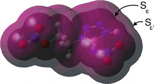
Figure 1. Surfaces of constant electron density for compound 1. The electron density on the outer surface is 0.0001 a.u., while it is 0.0040 a.u. on the inner. Both surfaces were computed with the B3LYP functional and a basis set of type 6-31G(d). The illustration was produced with the GaussView 4 software [13].

Given the assumption that a property is to some extent determined by non-covalent intermolecular interactions, workers have restricted to a particular surface , extracting statistical quantities deemed relevant for predicting said property. The properties modelled by this procedure include impact sensitivities [10,11], critical and boiling points [14], sublimation enthalpies and solvation free energies [1], solubilities [12,15], partition coefficients [16], crystal densities [5,8] and the potency of inhibitors as anti-HIV agents [17,18]. In general, it is assumed that there exists a function f, known as a general interaction properties function (GIPF) [4], such that (3) where the Φ⁽ⁱ⁾ are parameters extracted from restricted to the molecular surface. The objective of the developers of the GIPF procedure was to find means of making satisfactory predictions for properties of practical interest with a particular focus on molecular surfaces. In spite of the fact that it appears that a reasonable accuracy has been obtained in many cases, competing models f have often been left non-validated and judged solely by their ability to fit the data, regardless of complexity [4,9–11,14,16,17,19]. It is good practice to validate models, for instance by performing cross-validation or boot-strapping [20]. If validation is not possible, models of differing complexity are often compared by information criteria, which favour parsimonious models [21]. Given the fact that many of the GIPF models are very flexible (allowing several variables) and hence, vulnerable to overfitting, it is important that they are tested on unseen data-sets. Adopting the practice of validation will be beneficial to the further study of the effectiveness of these models.

Our work addresses a more general issue: if a model f is proposed whose parameters Φ⁽ⁱ⁾ are computed on the molecular surface , the choice of ε should be of minor or no importance, provided one stays within the as-yet unknown range [ε_min, ε_max] yielding adequate representations of the molecular surface. That is, if the parameters were computed on a different molecular surface, say , the predictions made by the model should not change. While others have remarked that the particular choice of electron density should be of minor importance [1,17,18], the mathematical consequences of this claim have not been investigated. Exploring these consequences is the subject of this paper.

In the special case of a linear single-variable model f, requiring that predictions remain the same on and is mathematically equivalent to demanding the existence of constants α, β, α′, β′, such that (4a) (4b)

In these equations, Φ_i(ε) is the parameter Φ computed on the surface of molecule i. Substituting Equation (4b(4b) ) into Equation (4a(4a) ), we find that (5) with and . We have discovered that if predictions are surface-invariant, then the parameter values of Φ computed on different surfaces must be linearly related to each other. Of particular interest is the contrapositive variant of this statement: if Equation (5(5) ) is false, then the predictions will differ on the two surfaces, i.e. Equations (4a(4a) ) and (4b(4b) ) cannot be true simultaneously. This means that parameters Φ which violate the linearity of Equation (5(5) ) should never be used in linear single-variable models. We will refer to the requirement that parameters satisfy Equation (5(5) ) as the principle of molecular surface invariance.

In order to illustrate the usefulness of the principle, we will study two aspects of : the variation of and the imbalance of positive and negative values of . It has been argued that variation is a measure of ‘local polarity’, thus being a prerequisite for intermolecular interactions [22], and that imbalance renders favourable interactions less probable [1,4,7]. We will study the following two parameters quantifying variation:¹ (6a) (6b)

Both Π and σ are measures of the spread about the mean. Here, N is the number of points on the discretised molecular surface, and is the average potential value on the surface. Since its introduction by Brinck et al. [22], Π has been used to model octanol/water partition coefficients [16], enzyme inhibition concentrations [17,18], crystal densities [5,7,8,23], impact sensitivities [4] and solute-induced frequency shifts [9]. As we wish to study aspects of in general, rather than investigating particular parameters, we consider σ as an analogue of the frequently used Π. Similarly, to quantify imbalance, we study the following parameters: (7a) (7b)

In Equation (7a(7a) ), σ²₋ and σ²₊ are variances of on the parts of the molecular surface for which is negative and positive, respectively. It should be noted that σ²₋ = σ₊² (signifying balance) implies ν = 0.25, while σ²₋ ≠ σ₊² (signifying imbalance) implies ν < 0.25. The imbalance parameter ν has been used to model crystal densities [7,8], enzyme inhibition concentrations [17,18], impact sensitivities [10], boiling and critical points [14] and solubilities [4]. We treat Θ as an analogue to ν. To understand the reasoning leading to Θ, consider the coefficient of skewness [24], (8) We claim that imbalance is adequately represented by the ‘absolute skewness about zero’. To obtain a measure of this, we first replaced by zero (denoting the resulting quantity by s′) and then took its absolute value (Θ = |s′|). In a recent paper, we studied the role of variation (σ, Π) and imbalance (ν, Θ) in the prediction of crystal densities [23].

Both Π and ν have been applied to model the impact sensitivity of a material, as given by h₅₀, the height at which 50 per cent of samples detonate, and I₅₀, the impact energy at which 50 per cent of samples detonate [4,10], (9) (10) It should be kept in mind that these models have multiple variables, and consequently that the linearity of Equation (5(5) ) is not strictly required for the invariance of predictions.

2. Procedure

A set of 44 compounds were considered, most of them comprised of carbon, hydrogen, nitrogen and oxygen, but some also contain chlorine, fluorine, phosphorous or sulphur. An overview of the studied molecules is given in Table 1.

Table 2. Tolerances applied to identify points on the studied molecular surfaces.

Surface
Tolerance [10^−4a.u.]	0.1	0.5	1	2	3

Table 1. Overview of studied compounds, their ν and Π values on the surfaces , and . The quantity Π is listed in units of Hartree, ν is dimensionless.

Formula	Nr.	CAS-ID	ν0.0001	ν0.0010	ν0.0040	Π0.0001	Π0.0010	Π0.0040
C3H5N7O5	1	1334230-65-7	0.25	0.24	0.20	0.018	0.026	0.036
C5H7N3O5S	2	1310420-43-9	0.23	0.25	0.23	0.027	0.036	0.044
C10H18O6	3	1310054-86-4	0.25	0.25	0.24	0.014	0.021	0.029
C3H6N6O3	4	1308657-70-6	0.24	0.24	0.22	0.022	0.031	0.040
C13H9ClN4O	5	1313411-75-4	0.25	0.24	0.25	0.011	0.015	0.021
C4H5N3O4S	6	1310420-42-8	0.25	0.23	0.21	0.027	0.036	0.044
C3HN7O8	7	1286279-08-0	0.13	0.11	0.09	0.016	0.023	0.033
C3H6N4O8	8	1255215-40-7	0.14	0.13	0.10	0.019	0.026	0.035
C4H4N8	9	1240554-70-4	0.22	0.24	0.25	0.016	0.023	0.032
C13H11Cl2N3	10	1224197-56-1	0.25	0.25	0.24	0.017	0.022	0.027
C5H9N5O8	11	1195678-79-5	0.22	0.19	0.15	0.016	0.025	0.034
C7H10N2O3S	12	1195693-61-8	0.25	0.24	0.22	0.025	0.032	0.041
C12H9Cl2NO3	13	50471-44-8	0.25	0.25	0.24	0.011	0.016	0.022
C8H3Cl2NO4	14	24564-72-5	0.16	0.22	0.25	0.010	0.015	0.022
C14H10N2O2	15	5585-14-8	0.14	0.19	0.24	0.011	0.015	0.020
C9H8N2	16	1126-00-7	0.20	0.23	0.25	0.010	0.015	0.021
C12H7N7O6	17	1198599-44-8	0.23	0.22	0.20	0.017	0.024	0.034
C4H6N12O4	18	1135076-68-4	0.22	0.20	0.18	0.019	0.027	0.037
C2H3N5O2	19	1163729-75-6	0.24	0.21	0.18	0.020	0.027	0.037
C10H8O	20	135-19-3	0.22	0.19	0.15	0.011	0.017	0.022
C3H3N9O2	21	212318-72-4	0.20	0.18	0.15	0.023	0.032	0.042
C6H2N2O8	22	479-22-1	0.19	0.15	0.10	0.021	0.030	0.041
C6H10N6O2	23	1135076-65-1	0.22	0.25	0.25	0.014	0.020	0.027
C12H16N2	24	1117789-09-9	0.14	0.16	0.20	0.019	0.025	0.031
C6H7N5O	25	1071952-90-3	0.20	0.22	0.25	0.022	0.030	0.037
C12H11NO3	26	86311-67-3	0.10	0.13	0.20	0.011	0.015	0.020
C12H18N4S	27	83277-80-9	0.22	0.21	0.24	0.011	0.015	0.019
C4H6N6O8	28	81360-42-1	0.11	0.10	0.08	0.017	0.026	0.036
C6H8NO3P	29	80241-43-6	0.25	0.25	0.24	0.015	0.023	0.031
C7H9NOS	30	77555-27-2	0.24	0.25	0.25	0.012	0.017	0.023
C13H9N	31	229-87-8	0.18	0.22	0.24	0.010	0.015	0.019
C8H6O4	32	121-91-5	0.25	0.24	0.23	0.012	0.018	0.024
C6H4N2O5	33	51-28-5	0.24	0.25	0.23	0.015	0.022	0.030
C10H16O5	34	1338212-46-6	0.17	0.20	0.24	0.014	0.020	0.028
C8H6O4	35	100-21-0	0.25	0.24	0.23	0.012	0.017	0.025
C15H16O2	36	80-05-7	0.21	0.19	0.18	0.010	0.015	0.021
C9H5N5O6	37	23309-22-0	0.23	0.21	0.19	0.017	0.026	0.036
C6H4N2O2	38	23296-57-3	0.22	0.25	0.25	0.013	0.018	0.025
C9H9NO3	39	19182-97-9	0.17	0.22	0.25	0.015	0.021	0.028
CH2N6O2	40	18588-16-4	0.23	0.19	0.16	0.021	0.031	0.041
C8H4N6O6	41	18373-83-6	0.18	0.18	0.15	0.017	0.025	0.035
C5H5ClN2O	42	17551-52-9	0.22	0.22	0.25	0.019	0.025	0.035
C5H6N2O2	43	17325-26-7	0.24	0.25	0.25	0.013	0.020	0.029
C4H2N4O2	44	17098-88-3	0.24	0.25	0.24	0.017	0.026	0.034

All computations were performed with the GAUSSIAN03 Revision E.01 software [25]. The molecular geometries were optimised with density functional theory (DFT), applying the B3LYP functional and basis sets of type 6-31G(d). Both n(r) and were computed on a 100 by 100 by 100 grid. The statistical quantities Π, σ, ν and Θ were obtained manually on the five molecular surfaces , , , and . Points were identified as being on the surface with tolerances producing 4000–10,000 points on each surface, depending on the size of the molecule, see Table 2.

3. Results and discussion

Having computed Φ = Π, σ, ν and Θ on five molecular surfaces, each parameter was compared with its value on the commonly used surface . The rate at which linearity deteriorates may, thus, be taken to indicate how far away from the conventional molecular surface one must stray before the models cease to yield consistent predictions. The results for the measures of spread and imbalance are given in Figures 2 and 3, respectively.

Figure 2. The parameter values of Π and σ on the isosurfaces , , , and . Both Π and σ are given in units of Hartree.

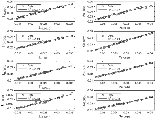
Figure 3. The parameter values of ν and Θ on the isosurfaces , , , and .

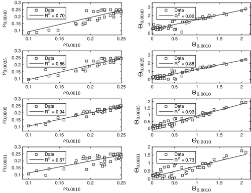
It is evident from these figures that imbalance (quantified by ν and Θ) does not satisfy the linearity in Equation (5(5) ). We conclude that imbalance should never be used in linear single-variable models, i.e. models of the form (11) We have, in fact, shown that such a model cannot make the same predictions on all molecular surfaces. Inconsistent predictions in single-variable models does not preclude the possibility of consistent predictions in multi-variable models, a particular example of which is given in Equation (10(10) ). For this to be true, it seems that some highly non-trivial cancellation is required between the many parameters. At the very least, our results serve as a warning against such models, since the imbalance does not give consistent predictions for even the simplest of cases, that of a single variable. One may rightly object that ν and Θ could be improper measures of imbalance. We note, however, that they are in fair agreement, see Figure 4. A symmetric distribution should imply Θ = 0 and ν = 0.25, while asymmetry should increase Θ and reduce ν. This is consistent with our findings.

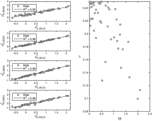
Figure 4. Left: the parameter values of s′ on the isosurfaces , , , and . Right: the imbalance quantities Θ and ν.

Having shown that measures of imbalance fail to satisfy surface-invariance, we proceed to ascertain the severity of the inconsistency, i.e. to analyse to what extent it is expected to cause different predictions on different surfaces. Observe that from the lower right plot of Figure 3 one readily identifies two compounds A and B for which, approximately, (12) Although these molecules have identical Θ values on , their values differ markedly on . The difference is significant, as is confirmed from the fact that Θ ∈ [0, 2] on . Thus, ΔΘ = 1 covers half the range of Θ values in the study, clearly causing inconsistent predictions for A and B in models of the form property = α Θ + γ. In terms of impact sensitivity, A and B will be of equal and small sensitivity according to , whereas A will be stable and B moderately sensitive on . We conclude that the use of imbalance parameters in linear models will result in significantly inconsistent predictions.

Interestingly, while measures of imbalance do not satisfy the linearity of Equation (5(5) ), the skewness s′ does, see Figure 4. The problem with imbalance is, thus, revealed to be that it treats left- and right-skewness on an equal footing. Both of them signify imbalance.

Whereas imbalance produces non-linearities, the measures of spread satisfy the linearity to a high degree (R² ≥ 0.97). The implication is that this aspect of is not inconsistent with its use in linear models. These results do not, however, imply that variation is relevant for predicting chemical or physical properties, only that applying it does not lead to any contradictions.

Considering the choice of electron density range, we note the similarity and proximity of and , see Figure 1. Moreover, the trends shown by the electrostatic potential suggest that the information contained in the parameters of variation (σ, Π) and skewness (s′) is preserved in the electron density range studied. Murray et al. have given a similar statement for the 0.0010 to 0.0050 a.u. range [26]. The appropriate values for ε_min and ε_max remain, however, an open question that will require more research to settle.

Earlier studies have considered the invariance of predictions on different molecular surfaces. Murray et al. [27] studied a model for the hydrogen-bond-acceptor parameter β. The molecular electrostatic spatial minima V_{S, min} and maxima V_{S, max} were used as parameters. By analysing their data (see tables 1 and 2 in [27]), we found that these parameters satisfy the principle of molecular surface invariance in Equation (5(5) ) on the three surfaces , and . Murray et al. [26] investigated the use of local ionisation energy as a tool for identifying reactive sites on defect-containing model graphene systems. The positions at which the local ionisation energy has a minimum were of particular interest since these sites are indicative of the locations of the least tightly bound, most reactive electrons. Considering their data (see table 4 in [26]), we found that the surface-minimum of the local ionisation energy fulfills the principle on , and .

Instead of focusing on particular models (with one or more parameters), our approach is to consider the parameters themselves and ask whether the predictions of any model using these parameters will be similar on different surfaces. The advantage of this approach is that it allows one to rigorously weed out parameters that should probably be avoided in all models. Constructing new models with parameters that satisfy molecular surface invariance is necessary for the predictions to remain the same on a range of surfaces.

4. Conclusions and summary

The arbitrary choice of the molecular surface has its pitfalls, especially in the context of modelling. While it is reasonable to define such a surface by regions of constant and small electron density, one is still left with having to choose a particular value. An essential question is how improbable the detection of an electron should be in order to be on the ‘surface’. We take the view that there must be many equivalent choices, all equally well suited to represent the surface.

An appealing idea is to study the electrostatic potential on the molecular surface. Perhaps information of intermolecular interactions may be extracted, perhaps this information is relevant for a range of physical and chemical properties. Pursuing this idea, several workers have suggested models of the form (13) where Φ(ε) is the value of Φ on the surface of electron density ε. (These models often have several parameters Φ, but this is not important in the present discussion.) These efforts have in common that the importance of the particular choice of electron density ε has been overlooked. Our main claim is that there exists a range of electron densities whose corresponding surfaces are all equivalent representations of the molecular surface. Consequently, no model should make different predictions on different surfaces.

We proved that if linear single-variable models are to make the same predictions on every molecular surface, Φ(ε) must be linearly related to Φ(ε′), where ε and ε′ are electron densities corresponding to valid molecular surfaces. If this linearity is violated, no model of the form of Equation (13(13) ) is able to yield the same predictions on the two surfaces.

To illustrate the use of this requirement, we have demonstrated that imbalance, i.e. the predominance of negative or positive electrostatic potential on the surface, violates the linearity requirement in the electron density range [0.0001 a.u., 0.0040 a.u.]. Thus, any linear single-variable model applying this aspect will not produce consistent results on surfaces within this range. Moreover, we have demonstrated that the differences in predictions will in many cases be significant, and hence, that the violation of linearity is not merely a mathematical nuance. We also argue that multi-variable models applying imbalance should be avoided, reasoning that consistent predictions in this case will require highly non-trivial cancellations between the parameters making up the model. In the literature, linear models applying imbalance have been proposed to predict enzyme inhibition concentrations [18], impact energies [10], potencies of anti-HIV agents [17] and solubilities [4]. Our work indicates that none of these models should be used, since their predictions are expected to become inconsistent with slight changes in the molecular surface. This in turn suggests that the observed trends in the aforementioned studies might be coincidental. In another study, we have shown that this appears to be the case in the prediction of crystal densities [23].

In our consideration of imbalance and variation parameters, we have implicitly assumed that the range of electron densities [0.0001 a.u., 0.0040 a.u.] adequately represents the molecular surface. This appears to be a valid assumption, given that the information contained in the variation parameters (Π, σ) and the skewness parameter (s′) is preserved throughout the range of electron densities.

We recommend that all molecular surface-based parameters should be checked for linearity, in the sense of Equation (5(5) ), before being considered as a relevant quantity in linear modelling of physical and chemical properties. In these modelling efforts, better predictive power may be obtained by using model parameters that are invariant to the change of molecular surface. As a final remark, we emphasise that these considerations are not restricted to the use of the electrostatic potential, but remain valid for any parameter obtained from the surface of molecules.

Disclosure statement

No potential conflict of interest was reported by the authors.

Notes

1. We used the unbiased estimator for σ in our calculations, dividing by N − 1 instead of N. Since N > 4000 in all calculations, this makes no difference. We wrote N for readability.

References

- P. Politzer and J.S. Murray, Theor. Chem. Acc. 108 (3), 134–142 (2002).
- R.F.W. Bader, M.T. Carroll, J.R. Cheeseman, and C. Chang, J. Am. Chem. Soc. 109 (26), 7968–7979 (1987).
- A.F. Jalbout, Z.Y. Zhou, X. Li, M. Solimannejad, and Y. Ma, Comput. Theor. Chem. 664–665, 15 (2003).
- J.S. Murray, T. Brinck, P. Lane, K. Paulsen, and P. Politzer, Comput. Theor. Chem. 307, 55 (1994).
- P. Politzer, J. Martinez, J.S. Murray, M.C. Concha, and A. Toro-Labbé, Mol. Phys. 107 (19), 2095–2101 (2009).
- B.M. Rice, J.J. Hare, and E.F.C. Byrd, J. Phys. Chem. A 111 (42), 10874–10879 (2007).
- P. Politzer, J. Martinez, J.S. Murray, and M.C. Concha, Mol. Phys. 108 (10): 1391–1396 (2010).
- B.M. Rice and E.F.C. Byrd, J. Comput. Chem. 34 (25), 2146–2151 (2013).
- H. Hagelin, J.S. Murray, P. Politzer, T. Brinck, and M. Berthelot, Can. J. Chem. 73 (4), 483–488 (1995).
- J.S. Murray, M.C. Concha, and P. Politzer, Mol. Phys. 107 (1), 89–97 (2009).
- J.S. Murray, P. Lane, and P. Politzer, Mol. Phys. 93 (2), 187–194 (1998).
- P. Politzer, J.S. Murray, P. Lane, and T. Brinck, J. Phys. Chem. 97 (3), 729–732 (1993).
- R. Dennington II, T. Keith, and J. Millam, GaussView Version 4.1 (Semichem, Inc. Shawnee Mission, KS, 2007).
- J.S. Murray, P. Lane, T. Brinck, K. Paulsen, M.E. Grice, and P. Politzer, J. Phys. Chem. 97 (37), 9369–9373 (1993).
- P. Politzer, P. Lane, J.S. Murray, and T. Brinck, J. Phys. Chem. 96 (20), 7938–7943 (1992).
- T. Brinck, J.S. Murray, and P. Politzer, J. Org. Chem. 58 (25), 7070–7073 (1993a).
- P. Politzer, J.S. Murray, and Z. Peralta-Inga, Int. J. Quantum Chem. 85 (6), 676–684 (2001).
- T. Brinck, P. Jin, Y. Ma, J.S. Murray, and P. Politzer, J. Mol. Model. 9 (2), 77–83 (2003).
- T. Brinck, J.S. Murray, and P. Politzer, Int. J. Quantum Chem. 48 (2), 73–88 (1993).
- R. Wehrens, Chemometrics with R: Multivariate Data Analysis in the Natural Sciences and Life Sciences (Springer, Heidelberg, 2011).
- K.P. Burnham and D.R. Anderson, Sociol. Methods Res. 33 (2), 261–304 (2004).
- T. Brinck, J.S. Murray, and P. Politzer, Mol. Phys. 76 (3), 609–617 (1992).
- E.F. Kjønstad, J.F. Moxnes, T.L. Jensen, and E. Unneberg, Mol. Phys., (2016) (submitted).
- G.A. Korn and T.M. Korn, Mathematical Handbook for Scientists and Engineers: Definitions, Theorems, and Formulas for Reference and Review (Dover Publications, New York, NY, 2000).
- M.J. Frisch, G.W. Trucks, H.B. Schlegel, G.E. Scuseria, M.A. Robb, J.R. Cheeseman, J.A. Montgomery, Jr., T. Vreven, K.N. Kudin, J.C. Burant, J.M. Millam, S.S. Iyengar, J. Tomasi, V. Barone, B. Mennucci, M. Cossi, G. Scalmani, N. Rega, G.A. Petersson, H. Nakatsuji, M. Hada, M. Ehara, K. Toyota, R. Fukuda, J. Hasegawa, M. Ishida, T. Nakajima, Y. Honda, O. Kitao, H. Nakai, M. Klene, X. Li, J.E. Knox, H.P. Hratchian, J.B. Cross, V. Bakken, C. Adamo, J. Jaramillo, R. Gomperts, R.E. Stratmann, O. Yazyev, A.J. Austin, R. Cammi, C. Pomelli, J.W. Ochterski, P.Y. Ayala, K. Morokuma, G.A. Voth, P. Salvador, J.J. Dannenberg, V.G. Zakrzewski, S. Dapprich, A.D. Daniels, M.C. Strain, O. Farkas, D.K. Malick, A.D. Rabuck, K. Raghavachari, J.B. Foresman, J.V. Ortiz, Q. Cui, A.G. Baboul, S. Clifford, J. Cioslowski, B.B. Stefanov, G. Liu, A. Liashenko, P. Piskorz, I. Komaromi, R.L. Martin, D.J. Fox, T. Keith, M.A. Al-Laham, C.Y. Peng, A. Nanayakkara, M. Challacombe, P.M.W. Gill, B. Johnson, W. Chen, M.W. Wong, C. Gonzalez, and J.A. Pople, Gaussian 03, Revision E.01 (Gaussian, Inc., Wallingford, CT, 2007).
- J.S. Murray, Z.P. Shields, P. Lane, L. Macaveiu, and F.A. Bulat, J. Mol. Model. 19 (7), 2825–2833 (2013).
- J.S. Murray, T. Brinck, M.E. Grice, and P. Politzer, J. Mol. Struct. THEOCHEM 256, 29 (1992).