A reduced basis approach for calculation of the Bethe–Salpeter excitation energies by using low-rank tensor factorisations^*

* Dedicated to Prof. Andreas Savin on occasion of his 65th birthday.

ABSTRACT

The Bethe–Salpeter equation (BSE) is a reliable model for estimating the absorption spectra in molecules and solids on the basis of accurate calculation of the excited states from first principles. Direct diagonalisation of the BSE matrix is practically intractable due to O(N⁶) complexity scaling in the size of the atomic orbital basis set, N. In this paper, we introduce and analyse a reduced basis approach to computation of the Bethe–Salpeter excitation energies which can lead to a relaxation of the numerical costs down to O(N³). The BSE operator is specified in terms of the two-electron integrals in the Hartree–Fock molecular orbital basis and the respective energies, calculated by the tensor-based solver described in previous works. The reduced basis method includes two steps. First, the diagonal plus low-rank approximation to fully populated blocks in the BSE matrix is calculated, enabling an easier partial eigenvalue solver for a large auxiliary system relying only on matrix–vector multiplications with rank-structured matrices. Second, a small subset of eigenvectors from the auxiliary eigenvalue problem is selected to build a projection of the exact BSE system onto this reduced basis set. Numerical tests demonstrate the ϵ-rank bounds for the blocks of the BSE matrix on examples of some compact molecules. The accuracy of the reduced basis approach vs. the effective matrix rank is illustrated.

GRAPHICAL ABSTRACT

KEYWORDS:

• Bethe–Salpeter equation
• Hartree–Fock equation
• two-electron integrals
• low-rank tensor decompositions
• model reduction
• reduced basis
• truncated Cholesky factorisation

AMS Subject Classification:

• 65F30
• 65F50
• 65N35
• 65F10

1. Introduction

In modern material science, there is a growing interest to ab initio computation of the absorption spectra for molecules or surfaces of solids. This computational problem can be treated either by using the time-dependent density functional theory (TD-DFT) [1–6] or by solving the Bethe–Salpeter equation (BSE) [7,8] based on the Green's function formalism and many-body perturbation theory [9–13]. A specific choice of the approximate computational model may depend on many physical and implementation aspects, see [9] for the detailed discussion. In particular, the BSE approach leads to the challenging numerical task concerning the solution of large eigenvalue problem for a dense matrix that, in general, is non-symmetric.

In the present paper, we consider the computational aspects of the large-scale algebraic BSE spectral problem when using the data-sparse matrix structures. We follow the particular formulation of the BSE problem based on the non-interacting Green's function via representation in terms of the Hartree–Fock (HF) molecular orbitals (MOs) [14,15], where it was applied to H₂ molecule in the minimal basis of two Slater functions.¹In the framework of this specific BSE formulation, we focus on the algebraic aspects of solving the computationally extensive spectral problems arising in the case of larger molecular systems. It is demonstrated that this scheme becomes practically applicable to moderate-size molecules when using tensor-structured HF calculations [16–19], accomplished by efficient representation of the two-electron integrals (TEI) in the MO basis in the form of a low-rank Cholesky factorisation [17,20]. In this way, the low-rank representation of the TEI tensor stipulates the beneficial structure of the BSE matrix blocks, thus enabling numerical algorithms of reduced complexity.

It is worth to note that the size of the BSE matrix scales quadratically with the size of the atomic orbital (AO) basis set, O(N²_b), used in ab initio HF calculations. The direct diagonalisation is limited by the O(N⁶_b) complexity, making the problem computationally expensive already for moderately sized molecules with a basis size N_b ≈ 100. Hence, a procedure that relies entirely on multiplication of the governing BSE matrix, or its approximation, with vectors (in the framework of some iterative procedure) is the only viable approach. In turn, fast matrix computations can be based on the use of low-rank representations since such data structures allow efficient storage and fast algebraic operations with linear complexity scaling in the matrix size.

Methods for solving partial eigenvalue problems for matrices with the special structure as in the BSE eigenvalue problem have been intensively studied in the literature. These structures are related to the so-called Hamiltonian matrices, exposing a particular block structure. Papers and books treating Hamiltonian eigenvalue problems include [21–25]; see also the recent survey [26] and the references therein. Special cases of the BSE and other eigenvalue problems related to HF approximations lead to anti-block-diagonal Hamiltonian eigenproblems that can be solved by special techniques based on minimisation principles [27,28]. The algebraic structure of the BSE matrix is not that of a Hamiltonian matrix in the general case, but yields a so-called complex J-symmetric matrix. Theory and numerical solution of such eigenvalue problems are discussed in [29–33], where the particular instance of the BSE matrix is considered in [33]. Other partial eigensolvers tailored for electronic structure calculations are discussed in [34,35]. The reduced basis method for large-scale systems is described in [36].

In this paper, we study a reduced basis approach to the approximate numerical solution of the BSE eigenvalue problem based on model reduction via projection onto a reduced basis, which is constructed by using the eigenvectors of a simplified system matrix obeying a simpler data-sparse structure. The reduced basis method includes two steps. First, the diagonal plus low-rank approximation to the fully populated blocks in the BSE matrix is calculated, enabling an easier partial eigenvalue solver for a large auxiliary system relying only on matrix–vector multiplications with rank-structured matrices. Second, a small subset of eigenvectors from the auxiliary eigenvalue problem is selected to build the projection of the exact BSE system onto this reduced basis set.

The approximation error incurred by the reduced basis approach depending on the rank truncation parameters is investigated. Theoretical and numerical analysis on the existence of the low-rank approximation and the respective rank bounds for matrix blocks in the BSE system matrix are presented. One of the favourable features of the approach is the quadratic convergence rate in approximate excitation energies compared with the accuracy of the reduced basis set thresholded by a rank truncation parameter ϵ > 0 (see Remark 3.3).

The reduced basis approach applies to the BSE system with matrix blocks of size N_oN_v × N_oN_v, where N_o and N_v denote the number of occupied and virtual HF orbitals, respectively, such that N_b = N_o + N_v. Since in general, N_oN_v = O(N²_b), the direct numerical calculation of the matrix elements, based on the precomputed TEI tensor in the HF MO basis, has a storage and numerical cost of the order of O(N⁴_b).

The construction of the reduced basis and the preceding low-rank decomposition of matrix blocks in the Bethe–Salpeter kernel are motivated by the use of truncated Cholesky factorisation of the TEI matrix [17,20]. To that end, the BSE matrix blocks are represented in terms of the precomputed Cholesky factors in the HF MO basis. Along with the diagonal energy matrix, this constitutes the structured representations of the dielectric and response functions, as well as the static screened interaction matrix. Taking into account the rank decomposition of TEI, the above quantities tolerate the low-rank approximation up to a chosen threshold.²This yields the construction of a so-called simplified BSE matrix with a diagonal plus low-rank structure in the matrix blocks, thus admitting efficient storage and matrix–vector products. The reduced basis is obtained by calculating several of the lowest eigenvectors of the auxiliary eigenvalue problem for the simplified matrix. A projection of the exact BSE matrix onto the reduced basis set and diagonalisation of the arising small-size matrix completes the reduced basis scheme.

Numerical tests for single molecules and finite chains of hydrogen atoms indicate the convergence in the senior excitation energies by the increase of the separation ranks.

The rest of the paper is organised as follows. Section 2 recalls the truncated Cholesky decomposition scheme for low-rank factorisation of the TEI tensor in the HF MO basis, that is the building block in the construction of the BSE matrix. Section 3 describes the algebraic computational scheme for evaluation of the entries in the BSE matrix, analyses the low-rank structure in different matrix blocks and describes the reduced basis approach. Section 4 presents numerical tests for several compact and extended molecules demonstrating the computational features of the reduced basis method applied to the full BSE system as well as to simplified model by the so-called Tamm–Dancoff approximation (TDA).

2. Low-rank approximation of the two-electron integrals in Hartree–Fock calculus

2.1. Cholesky decomposition of the TEI matrix

The numerical treatment of the TEI tensor (also known as the electron repulsion integrals) is one of the bottlenecks in the numerical solution of the HF equation and in density function theory (DFT) calculations for large molecules [37].

Given the AO basis set ${\left\{g_{\mu }\right\}}_{1\le \mu \le N_b}$, $g_{\mu }\in H^1\left({\mathbb{R}}^3\right)$, the associated TEI tensor B = [b_μνλσ] [38] is defined entrywise by (2.1) $$\begin{array}{ccc}\hfill b_{\mu \nu \lambda \sigma }& =& {\int }_{{\mathbb{R}}^3}{\int }_{{\mathbb{R}}^3}\frac{g_{\mu }\left(x\right)g_{\nu }\left(x\right)g_{\lambda }\left(y\right)g_{\sigma }\left(y\right)}{\parallel x-y\parallel }dxdy,\hfill \\ & & \mu ,\nu ,\lambda ,\sigma \in \{1,...,N_b\}=:{\mathcal{I}}_b.\hfill \end{array}$$(2.1) The corresponding N²_b × N_b² TEI matrix over the large index set $\mathcal{I}\times \mathcal{J}$, $\mathcal{I}=\mathcal{J}={\mathcal{I}}_b\otimes {\mathcal{I}}_b$, with ${\mathcal{I}}_b:=\{1,...,N_b\}$, $$B=\mathrm{mat}\left(\mathbf{B}\right)=\left[b_{\mu \nu ;\lambda \sigma }\right]\in {\mathbb{R}}^{N_b^2\times N_b^2},$$is obtained by matrix unfolding of the tensor B = [b_μνλσ]. The matrix B is proven to be symmetric and positive definite ensuring application of the incomplete Cholesky decomposition [37,39–41]. The tensor-based HF solver [16,19] employs the efficient calculation of the Cholesky factors [17,20] in (2.2) $$B\approx L{L}^T,L\in {\mathbb{R}}^{N_b^2\times R_B},R_B=O\left(N_b\right),$$(2.2) where the adaptively chosen column vectors in B are calculated in an efficient way. This allows the partial decoupling of the index sets {μν} and {λσ}.

Notice that the Cholesky factorisation (2.2(2.2) $$B\approx L{L}^T,L\in {\mathbb{R}}^{N_b^2\times R_B},R_B=O\left(N_b\right),$$(2.2) ) can be written in the following index form: (2.3) $$b_{\mu \nu ;\lambda \sigma }\approx \sum _{k=1}^{R_B}{L}_k(\mu ;\nu )L_k(\sigma ;\lambda ),$$(2.3) where the second factor corresponds to the transposed matrix L^T_k. Here L_k = L_k(μ; ν), k = 1, …, R_B, denotes the N_b × N_b matrix unfolding of the column vector L(:, k) from the Cholesky factor $L\in {\mathbb{R}}^{N_b^2\times R_B}$.

Numerical experiments indicate that the truncated Cholesky decomposition with the separation rank O(N_b) ensures a satisfactory numerical precision ϵ > 0 of order 10⁻⁵ to 10⁻⁶. The refined rank estimate O(N_b|log ϵ|) was observed for every molecular system considered so far [17,20].

In the standard quantum chemical implementations in the Gaussian-type AO basis, the numerically confirmed rank bound, $\mathrm{rank}\left(B\right)\le C_B{N}_b$ (C_B is of order 1–10), allows to reduce the complexity of building up the Fock matrix F to O(N³_b), which is by far dominated by the computational cost for the exchange term K(D) (see Section 2.2 ).

2.2. Rank bounds for the TEI matrix V

The 2N_o-electron HF equation for N_o pairwise L²-orthogonal occupied electronic orbitals, ${\psi }_i:{\mathbb{R}}^3\to \mathbb{R}$, ${\psi }_i\in H^1\left({\mathbb{R}}^3\right)$, reads as [38] (2.4) $$\begin{array}{ccc}\hfill \mathcal{F}{\psi }_i\left(x\right)& :=& \left[-\frac{1}{2}\Delta +V_c\left(x\right)+V_H\left(x\right)+\mathcal{K}\right]{\psi }_i\left(x\right)\hfill \\ & =& {ϵ}_i{\psi }_i\left(x\right),{\int }_{{\mathbb{R}}^3}{\psi }_i{\psi }_{j}dx={\delta }_{ij},\hfill \end{array}$$(2.4) i, j = 1, …, N_o, where the nonlinear Fock operator $\mathcal{F}$ on the left-hand side includes the nuclear and Hartree potentials V_c(x) and V_H(x) as well as the integral exchange operator $\mathcal{K}$.

In HF calculations, the full HF operator $\mathcal{F}$ is represented in the basis set ${\left\{g_{\mu }\right\}}_{1\le \mu \le N_b}$, $g_{\mu }\in H^1\left({\mathbb{R}}^3\right)$, of Gaussian-type AOs. We consider the complete set of HF MOs $\{C_p\in {\mathbb{R}}^{N_b}\}$, i.e. the pth column vectors in the coefficients matrix $C\in {\mathbb{R}}^{N_b\times N_b}$, and the corresponding energies {ϵp}, p = 1, 2, …, Nb. The occupied MOs ψi are represented (approximately) by the coefficient matrix $C_o=\left[C_{\mu i}\right]\in {\mathbb{R}}^{N_b\times N_o}$ (submatrix of C) as ψi = ∑Nbμ = 1Cμigμ, i = 1, …, No.

The coefficients matrix $C\in {\mathbb{R}}^{N_b\times N_b}$ solves the nonlinear eigenvalue problem (2.5) $$\begin{array}{ccc}\hfill [H+J(D)+K(D\left)\right]C& =& SC\mathcal{E},\mathcal{E}=\mathrm{diag}({ϵ}_1,...,{ϵ}_{N_b}),\hfill \\ \hfill C^{T}SC& =& I_{N_b},\hfill \end{array}$$(2.5) where H is the core Hamiltonian matrix, S is the mass matrix and (2.6) $$\begin{array}{ccc}\hfill J{\left(D\right)}_{\mu \nu }& =& \sum _{\kappa ,\lambda =1}^{N_b}{b}_{\mu \nu ,\kappa \lambda }{D}_{\kappa \lambda },\hfill \\ \hfill K{\left(D\right)}_{\mu \nu }& =& -\frac{1}{2}\sum _{\kappa ,\lambda =1}^{N_b}{b}_{\mu \lambda ,\nu \kappa }{D}_{\kappa \lambda },\hfill \end{array}$$(2.6) with $D=2C_o{C}_o^T\in {\mathbb{R}}^{N_b\times N_b}$ denoting the rank-N_o symmetric density matrix.

In BSE calculations, the TEI tensor B = [b_μνλσ], corresponding to the AO basis set, is represented in the MO basis: (2.7) $$\begin{array}{ccc}\hfill \mathbf{B}\mapsto \mathbf{V}=\left[v_{iajb}\right]:& & v_{iajb}=\sum _{\mu ,\nu ,\lambda ,\sigma =1}^{N_b}{C}_{\mu i}{C}_{\nu a}{C}_{\lambda j}{C}_{\sigma b}{b}_{\mu \nu ,\lambda \sigma },\hfill \\ & & a,b,i,j\in \{1,...,N_b\}.\hfill \end{array}$$(2.7) The BSE calculations utilise the two subtensors of V specified by the index sets ${\mathcal{I}}_o:=\{1,...,N_o\}$ and ${\mathcal{I}}_v:=\{N_o+1,...,N_b\}$, with N_o denoting the number of occupied orbitals. The first subtensor is defined as in the MP2 calculations [17]: (2.8) $$\mathbf{V}=\left[v_{iajb}\right]:a,b\in {\mathcal{I}}_v,i,j\in {\mathcal{I}}_o,$$(2.8) while the second one lives on the extended index set: (2.9) $$\widehat{\mathbf{V}}=\left[{\widehat{v}}_{turs}\right]:r,s\in {\mathcal{I}}_v,t,u\in {\mathcal{I}}_o.$$(2.9)

In the following, {C_i} and {C_a} denote the sets of occupied and virtual orbitals, respectively. We shall also use the notation N_v = N_b − N_o, N_ov = N_oN_v.

Denote the associated matrix by $V=\left[v_{ia,jb}\right]\in {\mathbb{R}}^{N_{ov}\times N_{ov}}$ in case (2.8(2.8) $$\mathbf{V}=\left[v_{iajb}\right]:a,b\in {\mathcal{I}}_v,i,j\in {\mathcal{I}}_o,$$(2.8) ), and similar by $\widehat{V}=\left[{\widehat{v}}_{tu,rs}\right]\in {\mathbb{R}}^{N_o^2\times N_v^2}$ in case (2.9(2.9) $$\widehat{\mathbf{V}}=\left[{\widehat{v}}_{turs}\right]:r,s\in {\mathcal{I}}_v,t,u\in {\mathcal{I}}_o.$$(2.9) ). The straightforward computation of the matrix V by the above representations accounts for the dominating impact on the overall numerical cost of order O(N⁵_b) in the evaluation of the block entries in the BSE matrix. A method of complexity O(N⁴_b) based on the low-rank tensor decomposition of the matrix V on the full index set was described in [17].

It can be shown that the rank R_B = O(N_b) approximation to matrix B ≈ LL^T with the N × R_B Cholesky factor, L, allows to introduce the low-rank representation of the tensor V, and then to reduce the asymptotic complexity of calculations to O(N⁴_b) (see [17]). Indeed, let C_m be the mth column of the coefficient matrix $C=\left\{C_{\mu i}\right\}\in {\mathbb{R}}^{N_b\times N_b}$. Then, inserting (2.3(2.3) $$b_{\mu \nu ;\lambda \sigma }\approx \sum _{k=1}^{R_B}{L}_k(\mu ;\nu )L_k(\sigma ;\lambda ),$$(2.3) ) in (2.7(2.7) $$\begin{array}{ccc}\hfill \mathbf{B}\mapsto \mathbf{V}=\left[v_{iajb}\right]:& & v_{iajb}=\sum _{\mu ,\nu ,\lambda ,\sigma =1}^{N_b}{C}_{\mu i}{C}_{\nu a}{C}_{\lambda j}{C}_{\sigma b}{b}_{\mu \nu ,\lambda \sigma },\hfill \\ & & a,b,i,j\in \{1,...,N_b\}.\hfill \end{array}$$(2.7) ) in the case of (2.8(2.8) $$\mathbf{V}=\left[v_{iajb}\right]:a,b\in {\mathcal{I}}_v,i,j\in {\mathcal{I}}_o,$$(2.8) ) leads to (2.10) $$\begin{array}{ccc}\hfill v_{iajb}& =& \sum _{k=1}^{R_B}\sum _{\mu ,\nu ,\lambda ,\sigma =1}^{N_b}{C}_{\mu i}{C}_{\nu a}{C}_{\lambda j}{C}_{\sigma b}{L}_k(\mu ;\nu )L_k(\sigma ;\lambda )\hfill \\ & =& \sum _{k=1}^{R_B}\left(\sum _{\mu ,\nu =1}^{N_b}{C}_{\mu i}{C}_{\nu a}{L}_k(\mu ;\nu )\right)\left(\sum _{\lambda ,\sigma =1}^{N_b}{C}_{\lambda j}{C}_{\sigma b}{L}_k(\sigma ;\lambda )\right)\hfill \\ & =& \sum _{k=1}^{R_B}\left(C_i^T{L}_k{C}_a\right)\left(C_b^T{L}_k^T{C}_j\right)=\sum _{k=1}^{R_B}\left(C_i^T{L}_k{C}_a\right){\left(C_j^T{L}_k{C}_b\right)}^T.\hfill \end{array}$$(2.10) A similar factorisation can be derived in the case of (2.9(2.9) $$\widehat{\mathbf{V}}=\left[{\widehat{v}}_{turs}\right]:r,s\in {\mathcal{I}}_v,t,u\in {\mathcal{I}}_o.$$(2.9) ). The precise formulation is given by the following lemma [17], which will be used in further considerations.

Lemma 2.1:

Let the rank-R_B Cholesky decomposition of the matrix B be given by (2.2(2.2) $$B\approx L{L}^T,L\in {\mathbb{R}}^{N_b^2\times R_B},R_B=O\left(N_b\right),$$(2.2) ), then the matrix unfolding V = [v_{ia; jb}] corresponding to (2.8(2.8) $$\mathbf{V}=\left[v_{iajb}\right]:a,b\in {\mathcal{I}}_v,i,j\in {\mathcal{I}}_o,$$(2.8) ) allows a rank decomposition with $\mathrm{rank}\left(V\right)\le R_B$. The R_B-term representation of the matrix V = [v_{ia; jb}] takes the following form: $$V=L_V{L}_V^T,L_V\in {\mathbb{R}}^{N_{ov}\times R_B},$$where the columns of L_V are given by $$\begin{array}{c}\hfill L_V((i-1)N_{vir}+a-N_{orb};k)=C_i^T{L}_k{C}_a,\\ \hfill k=1,...,R_B,a\in {\mathcal{I}}_v,i\in {\mathcal{I}}_o.\end{array}$$On the index set (2.9(2.9) $$\widehat{\mathbf{V}}=\left[{\widehat{v}}_{turs}\right]:r,s\in {\mathcal{I}}_v,t,u\in {\mathcal{I}}_o.$$(2.9) ), we have $\widehat{V}=U_{\widehat{V}}{W}_{\widehat{V}}^T\in {\mathbb{R}}^{N_o^2\times N_v^2}$ with $U_{\widehat{V}}\in {\mathbb{R}}^{N_o^2\times R_B}$, $W_{\widehat{V}}\in {\mathbb{R}}^{N_v^2\times R_B}$.

The numerical cost is determined by the computation complexity and storage size for the factors L_V, $U_{\widehat{V}}$ and $W_{\widehat{V}}$ in the above rank-structured factorisations.

Lemma 2.1 provides the upper bounds on $\mathrm{rank}\left(V\right)$ in the representation (2.10(2.10) $$\begin{array}{ccc}\hfill v_{iajb}& =& \sum _{k=1}^{R_B}\sum _{\mu ,\nu ,\lambda ,\sigma =1}^{N_b}{C}_{\mu i}{C}_{\nu a}{C}_{\lambda j}{C}_{\sigma b}{L}_k(\mu ;\nu )L_k(\sigma ;\lambda )\hfill \\ & =& \sum _{k=1}^{R_B}\left(\sum _{\mu ,\nu =1}^{N_b}{C}_{\mu i}{C}_{\nu a}{L}_k(\mu ;\nu )\right)\left(\sum _{\lambda ,\sigma =1}^{N_b}{C}_{\lambda j}{C}_{\sigma b}{L}_k(\sigma ;\lambda )\right)\hfill \\ & =& \sum _{k=1}^{R_B}\left(C_i^T{L}_k{C}_a\right)\left(C_b^T{L}_k^T{C}_j\right)=\sum _{k=1}^{R_B}\left(C_i^T{L}_k{C}_a\right){\left(C_j^T{L}_k{C}_b\right)}^T.\hfill \end{array}$$(2.10) ) which might be reduced by the ϵ-rank truncation. It can be shown that the ϵ-rank of the matrix V remains of the same magnitude as that for the TEI matrix B obtained by its ϵ-rank truncated Cholesky factorisation (see the numerical illustration in Section 3.2).

Numerical tests in [17] indicate that the singular values of the TEI matrix B decay exponentially as (2.11) $${\sigma }_k\le C{e}^{-\frac{z}{N_b}k},$$(2.11) where the constant z > 0 depends weakly on the molecule configuration. If we define R_B(ϵ) as the minimal number satisfying the condition (2.12) $$\sum _{k=R_B\left(ϵ\right)+1}^{R_B}{\sigma }_k^2\le {ϵ}^2,$$(2.12) then the estimate (2.11(2.11) $${\sigma }_k\le C{e}^{-\frac{z}{N_b}k},$$(2.11) ) leads to the ϵ-rank bound R_B(ϵ) ≤ CN_b|log ϵ|, which will be postulated in the following discussion.

Our goal is to justify that R_V(ϵ) increases only logarithmically in ϵ, similar to the bound for R_B(ϵ). To that end, we introduce the singular value decomposition (SVD) decomposition of the matrix B, $$B=U{D}_B{U}^T,U\in {\mathbb{R}}^{N_b^2\times R_B},D_B\in {\mathbb{R}}^{R_B\times R_B},$$which can be written in the following index form: (2.13) $$b_{\mu \nu ;\lambda \sigma }=\sum _{k=1}^{R_B}{\sigma }_k{U}_k(\mu ;\nu )U_k(\sigma ;\lambda ),$$(2.13) with $U_k=\left[U_k(\mu ;\nu )\right]\in {\mathbb{R}}^{N_b\times N_b}$ and ‖U_k‖_F = 1, k = 1, …, R_B.

Lemma 2.2:

For given ϵ > 0, there exists a rank-r approximation V_r to the matrix V, and a constant C > 0 not depending on ϵ, such that r ≤ R_B(ϵ) and $$\parallel V_r-V\parallel \le C{N}_bϵ|logϵ|.$$

Proof.

We estimate the RB(ϵ)-term truncation error by using the representation (2.13(2.13) $$b_{\mu \nu ;\lambda \sigma }=\sum _{k=1}^{R_B}{\sigma }_k{U}_k(\mu ;\nu )U_k(\sigma ;\lambda ),$$(2.13) ), (2.14) $$\begin{array}{ccc}\hfill v_{iajb}& =& \sum _{k=1}^{R_B}{\sigma }_k\sum _{\mu ,\nu ,\lambda ,\sigma =1}^{N_b}{C}_{\mu i}{C}_{\nu a}{C}_{\lambda j}{C}_{\sigma b}{U}_k(\mu ;\nu )U_k(\sigma ;\lambda )\hfill \\ & =& \sum _{k=1}^{R_B}{\sigma }_k\left(\sum _{\mu ,\nu =1}^{N_b}{C}_{\mu i}{C}_{\nu a}{U}_k(\mu ;\nu )\right)\hfill \\ & & \times \left(\sum _{\lambda ,\sigma =1}^{N_b}{C}_{\lambda j}{C}_{\sigma b}{U}_k(\sigma ;\lambda )\right)\hfill \\ & =& \sum _{k=1}^{R_B}{\sigma }_k\left(C_i^T{U}_k{C}_a\right)\left(C_b^T{U}_k^T{C}_j\right)\hfill \\ & =& \sum _{k=1}^{R_B}{\sigma }_k\left(C_i^T{U}_k{C}_a\right){\left(C_j^T{U}_k{C}_b\right)}^T,\hfill \end{array}$$(2.14) which can be presented in the matrix form V = ∑RBk = 1σkVkVTk, where Vk(i; a) = CTiUkCa. By definition of RB(ϵ), we have (2.12(2.12) $$\sum _{k=R_B\left(ϵ\right)+1}^{R_B}{\sigma }_k^2\le {ϵ}^2,$$(2.12) ). Hence, the error of the rank-RB(ϵ) approximation defined by Vr = ∑RB(ϵ)k = 1σkVkVTk, can be bounded by (2.15) $$\begin{array}{ccc}\hfill ∥\sum _{k=R_B\left(ϵ\right)+1}^{R_B}{\sigma }_k{V}_k{V}_k^T∥& \le & {\left(\sum _{k=R_B\left(ϵ\right)+1}^{R_B}{\sigma }_k^2\right)}^{1/2}{\left(\sum _{k=R_B\left(ϵ\right)+1}^{R_B}{\parallel V_k\parallel }^4\right)}^{1/2}\hfill \\ & \le & ϵ{\left(\sum _{k=R_B\left(ϵ\right)+1}^{R_B}{\parallel V_k\parallel }^4\right)}^{1/2}\hfill \\ & \le & ϵ(R_B-R_B\left(ϵ\right)){\parallel C\parallel }_{{\mathcal{I}}_o}^2{\parallel C\parallel }_{{\mathcal{I}}_v}^2,\hfill \end{array}$$(2.15) taking into account that ‖Uk‖ = 1, k = 1, …, RB, and the Frobenius norm estimate $$\begin{array}{ccc}\hfill \parallel V_k{\parallel }^2& =& \parallel V_k{(i;a)\parallel }_F^2=\parallel C_i^T{U}_k{C}_a{\parallel }_F^2\le \parallel U_k{\parallel }^2\sum _{i,a}\parallel C_i{\parallel }^2{\parallel C_a\parallel }^2\hfill \\ & \le & \sum _{i\in {\mathcal{I}}_o}\parallel C_i{\parallel }^2\sum _{a\in {\mathcal{I}}_v}{\parallel C_a\parallel }^2\hfill \end{array}$$holds. We suppose that RB = O(Nb|log ϵ|), then the multiple of ϵ|log ϵ| in (2.15(2.15) $$\begin{array}{ccc}\hfill ∥\sum _{k=R_B\left(ϵ\right)+1}^{R_B}{\sigma }_k{V}_k{V}_k^T∥& \le & {\left(\sum _{k=R_B\left(ϵ\right)+1}^{R_B}{\sigma }_k^2\right)}^{1/2}{\left(\sum _{k=R_B\left(ϵ\right)+1}^{R_B}{\parallel V_k\parallel }^4\right)}^{1/2}\hfill \\ & \le & ϵ{\left(\sum _{k=R_B\left(ϵ\right)+1}^{R_B}{\parallel V_k\parallel }^4\right)}^{1/2}\hfill \\ & \le & ϵ(R_B-R_B\left(ϵ\right)){\parallel C\parallel }_{{\mathcal{I}}_o}^2{\parallel C\parallel }_{{\mathcal{I}}_v}^2,\hfill \end{array}$$(2.15) ) does not depend on ϵ, which proves our lemma.

The storage cost of these decompositions restricted to the active index set ${\mathcal{I}}_v\times {\mathcal{I}}_o$ amounts to R_V(ϵ)N_vN_o.

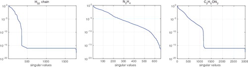
Figure 1 represents the singular values of the matrix V for H₃₂ chain, N₂H₄ and C₂H₅NO₂ (Glycine amino acid) molecules with the size of the basis set (N_b, N_o) equal to (128, 16), (82, 9) and (170, 20), respectively. They indicate that R_V(ϵ) is linearly proportional to |log ϵ|. Moreover, it is of the same order of magnitude as R_B(ϵ) (see [20]).

Figure 1. Decay of singular values of the matrix V for H₃₂-chain (1792 × 1792), N₂H₄ (657 × 657), and C₂H₅NO₂ (3000 × 3000) molecules. Size of V is given in brackets.

The calculation of V_r is based on the reduced truncated SVD algorithm applied to the initial rank-R_B Cholesky decomposition of the matrix V inherited from that for the TEI matrix B (see Lemma 2.1). Complexity of this straightforward computation on the active index set can be estimated by O(R²_BN_ov) = O(N²_bN_ov).

3. Tensor factorisation of the BSE matrix blocks

Here we discuss the main ingredients for calculation of blocks in the BSE matrix and their reduced rank approximate representation. We compose the 2N_ov × 2N_ov BSE matrix by Equations (46a) and (46b) in [14], though the construction of static screened interaction matrix w(ij, ab) in Equation (3.4(3.4) $$a_{ia,jb}:=\Delta {ϵ}_{ia,jb}+v_{ia,jb}-{\widehat{w}}_{ij,ab},$$(3.4) ) may slightly differ.

3.1. Tensor representations using TEI matrix in MTO basis

Construction of the BSE matrix includes computation of several auxiliary quantities. First, introduce a fourth-order diagonal ‘energy’ matrix by $$\Delta ϵ=\left[\Delta {ϵ}_{ia,jb}\right]\in {\mathbb{R}}^{N_{ov}\times N_{ov}}:\Delta {ϵ}_{ia,jb}=({ϵ}_a-{ϵ}_i){\delta }_{ij}{\delta }_{ab},$$that can be represented in the Kronecker product form $$\Delta ϵ=I_o\otimes \text{diag}\{{ϵ}_a:a\in {\mathcal{I}}_v\}-\text{diag}\{{ϵ}_i:i\in {\mathcal{I}}_o\}\otimes I_v,$$where I_o and I_v are the identity matrices on respective index sets. It is worth noting that if the so-called homo–lumo gap of the system is positive, i.e. $${ϵ}_a-{ϵ}_i>\delta >0,a\in {\mathcal{I}}_v,i\in {\mathcal{I}}_o,$$then the matrix $\Delta ϵ$ is invertible.

Using the matrix $\Delta ϵ$ and the N_ov × N_ov TEI matrix V = [v_{ia, jb}] represented in the MO basis as in (2.7(2.7) $$\begin{array}{ccc}\hfill \mathbf{B}\mapsto \mathbf{V}=\left[v_{iajb}\right]:& & v_{iajb}=\sum _{\mu ,\nu ,\lambda ,\sigma =1}^{N_b}{C}_{\mu i}{C}_{\nu a}{C}_{\lambda j}{C}_{\sigma b}{b}_{\mu \nu ,\lambda \sigma },\hfill \\ & & a,b,i,j\in \{1,...,N_b\}.\hfill \end{array}$$(2.7) ), the dielectric function (N_ov × N_ov matrix) Z = [z_{pq, rs}] is defined by $$z_{pq,rs}:={\delta }_{pr}{\delta }_{qs}-v_{pq,rs}{\left[{\chi }_0(\omega =0)\right]}_{rs,rs},$$with ${\chi }_0\left(\omega \right)$ being the matrix form of the so-called Lehmann representation to the response function. In turn, the matrix representation of the inverse of ${\chi }_0\left(\omega \right)$ is known to have the following form: $${\chi }_0^{-1}\left(\omega \right)=-\left(\begin{array}{cc}\hfill \Delta ϵ& \hfill \mathbf{0}\\ \hfill \mathbf{0}& \hfill \Delta ϵ\end{array}\right)+\omega \left(\begin{array}{cc}\hfill \mathbf{1}& \hfill \mathbf{0}\\ \hfill \mathbf{0}& \hfill -\mathbf{1}\end{array}\right),$$implying $${\chi }_0\left(0\right)=-\left(\begin{array}{cc}\hfill \Delta {ϵ}^{-1}& \hfill \mathbf{0}\\ \hfill \mathbf{0}& \hfill \Delta {ϵ}^{-1}\end{array}\right).$$

Let $\mathbf{1}\in {\mathbb{R}}^{N_{ov}}$ and ${\mathbf{d}}_{ϵ}=\text{diag}\left\{\Delta {ϵ}^{-1}\right\}\in {\mathbb{R}}^{N_{ov}}$ be the all-ones and diagonal vectors of $\Delta {ϵ}^{-1}$, respectively, specifying the rank-1 matrix 1⊗d_ϵ. In this notation, the matrix Z = [z_{pq, rs}] takes a compact form (3.1) $$Z=I_o\otimes I_v+V\odot \left(\mathbf{1}·{\mathbf{d}}_{ϵ}^T\right),$$(3.1) where ⊙ denotes the Hadamard product of matrices. Introducing the inverse matrix Z⁻¹, we finally define the so-called static screened interaction matrix (tensor) by (3.2) $$W=\left[w_{pq,rs}\right]:w_{pq,rs}:=\sum _{t\in {\mathcal{I}}_v,u\in {\mathcal{I}}_o}{z}_{pq,tu}^{-1}{v}_{tu,rs}.$$(3.2) In the forthcoming calculations, this equation should be considered on the conventional and extended index sets $\{p,s\in {\mathcal{I}}_o\}\times \{q,r\in {\mathcal{I}}_v\}$ and $\{p,q\in {\mathcal{I}}_o\}\times \{r,s\in {\mathcal{I}}_v\}$, respectively, such that v_{tu, rs} corresponds either to subtensor in (2.8(2.8) $$\mathbf{V}=\left[v_{iajb}\right]:a,b\in {\mathcal{I}}_v,i,j\in {\mathcal{I}}_o,$$(2.8) ) or in (2.9(2.9) $$\widehat{\mathbf{V}}=\left[{\widehat{v}}_{turs}\right]:r,s\in {\mathcal{I}}_v,t,u\in {\mathcal{I}}_o.$$(2.9) ).

Hence, on the conventional index set, we obtain the following matrix factorisation of W := [w_{ia, jb}]: $$W=Z^{-1}V\text{provided}\text{that}a,b\in {\mathcal{I}}_v,i,j\in {\mathcal{I}}_o,$$where V is calculated by (2.8(2.8) $$\mathbf{V}=\left[v_{iajb}\right]:a,b\in {\mathcal{I}}_v,i,j\in {\mathcal{I}}_o,$$(2.8) ). Lemma 2.1 suggests the existence of a low-rank factorisation for the matrix W defined above.

Lemma 3.1:

Let the matrix Z defined by (3.1(3.1) $$Z=I_o\otimes I_v+V\odot \left(\mathbf{1}·{\mathbf{d}}_{ϵ}^T\right),$$(3.1) ) over the index set $a,b\in {\mathcal{I}}_v,i,j\in {\mathcal{I}}_o$ be invertible. Then the rank of the respective matrix W = Z⁻¹V is bounded by $$rank\left(W\right)\le rank\left(V\right)\le R_B.$$

Proof.

Lemma 2.1 proves the representation $V=L_V{L}_V^T,L_V\in {\mathbb{R}}^{N_{ov}\times R_B}$, which ensures the rank-R_B factorisation $$W=Z^{-1}V=\left(Z^{-1}{L}_V\right)L_V^T,$$which can be calculated by solving linear system with structured data (see Section 3.2).

Furthermore, Equation (46a) in [14] includes matrix entries w_{ij, ab} for $a,b\in {\mathcal{I}}_v,i,j\in {\mathcal{I}}_o$. To this end, the modified matrix $\widehat{W}=\left[{\widehat{w}}_{pq,rs}\right]$ is computed by (3.2(3.2) $$W=\left[w_{pq,rs}\right]:w_{pq,rs}:=\sum _{t\in {\mathcal{I}}_v,u\in {\mathcal{I}}_o}{z}_{pq,tu}^{-1}{v}_{tu,rs}.$$(3.2) ) on the index set $\{p,q\in {\mathcal{I}}_o\}\times \{r,s\in {\mathcal{I}}_v\}$ by using entries ${\widehat{v}}_{ij,ab}$ in the matrix unfolding of the tensor $\widehat{\mathbf{V}}$ in (2.9(2.9) $$\widehat{\mathbf{V}}=\left[{\widehat{v}}_{turs}\right]:r,s\in {\mathcal{I}}_v,t,u\in {\mathcal{I}}_o.$$(2.9) ) multiplied from the left with the N²_o × N_o² submatrix of Z⁻¹.

Now the matrix representation of the BSE in the (ov, vo) subspace reads as the following eigenvalue problem determining the excitation energies ω_n: (3.3) $$F\left(\begin{array}{c}{\mathbf{x}}_n\\ {\mathbf{y}}_n\end{array}\right)\equiv \left(\begin{array}{cc}\hfill A& \hfill B\\ \hfill B^{*}& \hfill A^{*}\end{array}\right)\left(\begin{array}{c}{\mathbf{x}}_n\\ {\mathbf{y}}_n\end{array}\right)={\omega }_n\left(\begin{array}{cc}\hfill I& \hfill 0\\ \hfill 0& \hfill -I\end{array}\right)\left(\begin{array}{c}{\mathbf{x}}_n\\ {\mathbf{y}}_n\end{array}\right),$$(3.3) where the matrix blocks are defined in the index notation by (see (46a) and (46b) in [14] for more details): (3.4) $$a_{ia,jb}:=\Delta {ϵ}_{ia,jb}+v_{ia,jb}-{\widehat{w}}_{ij,ab},$$(3.4) (3.5) $$b_{ia,jb}:=v_{ia,bj}-w_{ib,aj},a,b\in {\mathcal{I}}_v,i,j\in {\mathcal{I}}_o.$$(3.5) In the matrix form, we obtain $$A=\Delta ϵ+V-\bar{W},$$where the matrix elements in $\bar{W}=\left[{\bar{w}}_{ia,jb}\right]$ are defined by ${\bar{w}}_{ia,jb}={\widehat{w}}_{ij,ab}$, computed by (3.2(3.2) $$W=\left[w_{pq,rs}\right]:w_{pq,rs}:=\sum _{t\in {\mathcal{I}}_v,u\in {\mathcal{I}}_o}{z}_{pq,tu}^{-1}{v}_{tu,rs}.$$(3.2) ) and (2.9(2.9) $$\widehat{\mathbf{V}}=\left[{\widehat{v}}_{turs}\right]:r,s\in {\mathcal{I}}_v,t,u\in {\mathcal{I}}_o.$$(2.9) ) as described above. Here the diagonal plus low-rank sparsity structure in $\Delta ϵ+V$ can be recognised in view of Lemma 2.1. For the matrix block B, we have $$B=\tilde{V}-\tilde{W}=V-\tilde{W},$$where the matrix $\tilde{V}$, corresponding to the partly transposed tensor, is defined entrywise by $$\tilde{\mathbf{V}}=\left[{\tilde{v}}_{iajb}\right]:=\left[v_{iabj}\right]=\left[v_{iajb}\right],$$thus coinciding with V in (2.8(2.8) $$\mathbf{V}=\left[v_{iajb}\right]:a,b\in {\mathcal{I}}_v,i,j\in {\mathcal{I}}_o,$$(2.8) ) due to the symmetry properties. Here $\tilde{W}$ is defined by permutation, $\tilde{W}=\left[{\tilde{w}}_{ia,jb}\right]=\left[w_{ib,aj}\right]$. In the following, we investigate the ϵ-rank structure in the matrix blocks A and B resulting from the corresponding factorisations of V.

Solutions of Equation (3.3(3.3) $$F\left(\begin{array}{c}{\mathbf{x}}_n\\ {\mathbf{y}}_n\end{array}\right)\equiv \left(\begin{array}{cc}\hfill A& \hfill B\\ \hfill B^{*}& \hfill A^{*}\end{array}\right)\left(\begin{array}{c}{\mathbf{x}}_n\\ {\mathbf{y}}_n\end{array}\right)={\omega }_n\left(\begin{array}{cc}\hfill I& \hfill 0\\ \hfill 0& \hfill -I\end{array}\right)\left(\begin{array}{c}{\mathbf{x}}_n\\ {\mathbf{y}}_n\end{array}\right),$$(3.3) ) come in pairs: excitation energies ω_n with eigenvectors (x_n, y_n), and de-excitation energies −ω_n with eigenvectors (x*_n, y_n*).

The block structure in the matrices A and B is inherited from the symmetry of the TEI matrix V, v_{ia, jb} = v*_{ai, bj} and the matrix W, w_{ia, jb} = w*_{bj, ai}. In particular, it is known from the literature that the matrix A is Hermitian and the matrix B is (complex) symmetric (since v_{ia, bj} = v_{jb, ai} and w_{ib, aj} = w_{ja, bi}), which we control in the matrix construction (see also [33] for implications on the algebraic properties of the BSE matrix).

In the following, we confine ourselves to the case of real spin orbitals, i.e. the matrices A and B remain real. It is known that for the real spin orbitals and if A + B and A − B are positive definite, the problem can be transformed into a half-size symmetric eigenvalue equation [3]. Indeed, in this case for every eigenpair, we have $$A\mathbf{x}+B\mathbf{y}=\omega \mathbf{x},B\mathbf{x}+A\mathbf{y}=-\omega \mathbf{y},$$implying $$\begin{array}{ccc}\hfill (A+B)(\mathbf{x}+\mathbf{y})& =& \omega (\mathbf{x}-\mathbf{y}),\hfill \\ \hfill (A-B)(\mathbf{x}-\mathbf{y})& =& \omega (\mathbf{x}+\mathbf{y}).\hfill \end{array}$$Now, if A + B and A − B are both positive definite, then the previous equations transform to (3.6) $$\begin{array}{c}\hfill M\mathbf{z}={\omega }^2\mathbf{z}\text{with}M={(A-B)}^{1/2}(A+B){(A-B)}^{1/2},\end{array}$$(3.6) with respect to the normalised eigenvectors $\mathbf{z}=\sqrt{\omega }{(A-B)}^{1/2}(\mathbf{x}+\mathbf{y})$. However, in this case the computation of the large fully populated matrix (A − B)^1/2 may become the bottleneck.

The dimension of the matrix in (3.3(3.3) $$F\left(\begin{array}{c}{\mathbf{x}}_n\\ {\mathbf{y}}_n\end{array}\right)\equiv \left(\begin{array}{cc}\hfill A& \hfill B\\ \hfill B^{*}& \hfill A^{*}\end{array}\right)\left(\begin{array}{c}{\mathbf{x}}_n\\ {\mathbf{y}}_n\end{array}\right)={\omega }_n\left(\begin{array}{cc}\hfill I& \hfill 0\\ \hfill 0& \hfill -I\end{array}\right)\left(\begin{array}{c}{\mathbf{x}}_n\\ {\mathbf{y}}_n\end{array}\right),$$(3.3) ) is 2N_oN_v × 2N_oN_v, where N_o and N_v denote the number of occupied and virtual orbitals, respectively. In general, N_oN_v is asymptotically of the size O(N²_b), i.e. the spectral problem (3.3(3.3) $$F\left(\begin{array}{c}{\mathbf{x}}_n\\ {\mathbf{y}}_n\end{array}\right)\equiv \left(\begin{array}{cc}\hfill A& \hfill B\\ \hfill B^{*}& \hfill A^{*}\end{array}\right)\left(\begin{array}{c}{\mathbf{x}}_n\\ {\mathbf{y}}_n\end{array}\right)={\omega }_n\left(\begin{array}{cc}\hfill I& \hfill 0\\ \hfill 0& \hfill -I\end{array}\right)\left(\begin{array}{c}{\mathbf{x}}_n\\ {\mathbf{y}}_n\end{array}\right),$$(3.3) ) may be computationally extensive. Indeed, the direct eigenvalue solver for (3.3(3.3) $$F\left(\begin{array}{c}{\mathbf{x}}_n\\ {\mathbf{y}}_n\end{array}\right)\equiv \left(\begin{array}{cc}\hfill A& \hfill B\\ \hfill B^{*}& \hfill A^{*}\end{array}\right)\left(\begin{array}{c}{\mathbf{x}}_n\\ {\mathbf{y}}_n\end{array}\right)={\omega }_n\left(\begin{array}{cc}\hfill I& \hfill 0\\ \hfill 0& \hfill -I\end{array}\right)\left(\begin{array}{c}{\mathbf{x}}_n\\ {\mathbf{y}}_n\end{array}\right),$$(3.3) ) (diagonalisation) becomes infeasible due to O(N⁶_b) complexity scaling. Furthermore, the numerical cost for calculation of the matrix elements based on the precomputed TEI integrals from the HF equation scales as O(N³_b)–O(N⁴_b), depending on how to compute the matrix W. Here, the low-rank structure in the matrix V can be adapted.

The challenging computational tasks arise in the case of lattice-structured compounds, where the number of basis functions increases proportionally to the lattice size L × L × L, i.e. N_b ∼ n₀L³, that quickly leads to intractable problems even for small lattices.

3.2. The reduced basis approach using low-rank approximations

The large matrix size in Equation (3.3(3.3) $$F\left(\begin{array}{c}{\mathbf{x}}_n\\ {\mathbf{y}}_n\end{array}\right)\equiv \left(\begin{array}{cc}\hfill A& \hfill B\\ \hfill B^{*}& \hfill A^{*}\end{array}\right)\left(\begin{array}{c}{\mathbf{x}}_n\\ {\mathbf{y}}_n\end{array}\right)={\omega }_n\left(\begin{array}{cc}\hfill I& \hfill 0\\ \hfill 0& \hfill -I\end{array}\right)\left(\begin{array}{c}{\mathbf{x}}_n\\ {\mathbf{y}}_n\end{array}\right),$$(3.3) ) makes the solution of the full eigenvalue problem computationally intractable even for moderate-size molecules, not to speak of lattice-structured compounds. Hence, in realistic quantum chemical simulations of excitation energies, the calculation of several (tens of) eigenpairs may be sufficient.

In the following, we show that the part $\Delta ϵ+V$ in the matrix block A has diagonal plus low-rank (DPLR) structure, while the submatrix $\tilde{V}$ in the block B exhibits low-rank approximability. Taking into account these structures, we propose a special partial eigenvalue problem solver based on the use of a reduced basis obtained from the eigenvectors of the reduced matrix that picks up only the essential part of the initial BSE matrix with the DPLR structure. The iterative solver is based on fast matrix–vector multiplication and efficient storage of all data involved in the computational scheme. Using the reduced basis approach, we then approximate the initial problem by its projection onto a reduced basis of moderate size.

We begin with the low-rank decomposition of the matrix V, $$V\approx L_V{L}_V^T,L_V\in {\mathbb{R}}^{N_{ov}\times R_V},R_V\le R_B,$$where the rank parameter R_V = R_V(ϵ) = O(N_b|log ϵ|) can be optimised depending on the truncation error ϵ > 0 (see [17] and Section 2.2).

First, we represent all matrix blocks and intermediate matrices included in the representation of the BSE matrix by using the above decomposition and diagonal matrices as follows. The properties of the Hadamard product imply that the matrix Z exhibits the representation $$Z=I_o\otimes I_v+L_V{L}_V^T\odot \left(\mathbf{1}·{\mathbf{d}}_{ϵ}^T\right)=I_{N_{ov}}+L_V{(L_V\odot {\mathbf{d}}_{ϵ})}^T,$$where the rank of the second summand does not exceed R_V. Hence, the linear system solver W = Z⁻¹V can be implemented by algorithms tailored to the DPLR structure by adapting the Sherman–Morrison formula.

The computational cost for setting up the full BSE matrix F in (3.3(3.3) $$F\left(\begin{array}{c}{\mathbf{x}}_n\\ {\mathbf{y}}_n\end{array}\right)\equiv \left(\begin{array}{cc}\hfill A& \hfill B\\ \hfill B^{*}& \hfill A^{*}\end{array}\right)\left(\begin{array}{c}{\mathbf{x}}_n\\ {\mathbf{y}}_n\end{array}\right)={\omega }_n\left(\begin{array}{cc}\hfill I& \hfill 0\\ \hfill 0& \hfill -I\end{array}\right)\left(\begin{array}{c}{\mathbf{x}}_n\\ {\mathbf{y}}_n\end{array}\right),$$(3.3) ) can be estimated by O(N²_ov), which includes the cost O(N_ovR_B) for generation the matrix V and the dominating cost O(N²_ov) for setting up $\bar{W}$.

In the following, we rewrite the spectral problem (3.3(3.3) $$F\left(\begin{array}{c}{\mathbf{x}}_n\\ {\mathbf{y}}_n\end{array}\right)\equiv \left(\begin{array}{cc}\hfill A& \hfill B\\ \hfill B^{*}& \hfill A^{*}\end{array}\right)\left(\begin{array}{c}{\mathbf{x}}_n\\ {\mathbf{y}}_n\end{array}\right)={\omega }_n\left(\begin{array}{cc}\hfill I& \hfill 0\\ \hfill 0& \hfill -I\end{array}\right)\left(\begin{array}{c}{\mathbf{x}}_n\\ {\mathbf{y}}_n\end{array}\right),$$(3.3) ) in the following equivalent form: (3.7) $$F_1\left(\begin{array}{c}{\mathbf{x}}_n\\ {\mathbf{y}}_n\end{array}\right)\equiv \left(\begin{array}{cc}\hfill A& \hfill B\\ \hfill -B^{*}& \hfill -A^{*}\end{array}\right)\left(\begin{array}{c}{\mathbf{x}}_n\\ {\mathbf{y}}_n\end{array}\right)={\omega }_n\left(\begin{array}{c}{\mathbf{x}}_n\\ {\mathbf{y}}_n\end{array}\right).$$(3.7)

The main idea of the reduced basis approach proposed in this paper is as follows. Instead of solving the partial eigenvalue problem for finding of, say, m₀ eigenpairs satisfying Equation (3.7(3.7) $$F_1\left(\begin{array}{c}{\mathbf{x}}_n\\ {\mathbf{y}}_n\end{array}\right)\equiv \left(\begin{array}{cc}\hfill A& \hfill B\\ \hfill -B^{*}& \hfill -A^{*}\end{array}\right)\left(\begin{array}{c}{\mathbf{x}}_n\\ {\mathbf{y}}_n\end{array}\right)={\omega }_n\left(\begin{array}{c}{\mathbf{x}}_n\\ {\mathbf{y}}_n\end{array}\right).$$(3.7) ), we first solve the slightly simplified auxiliary spectral problem with a modified matrix F₀. The approximation F₀ is obtained from F₁ by using low-rank approximations of the parts $\bar{W}$ and $\tilde{W}$ of the matrix blocks A and B, respectively, i.e. A and B are replaced by (3.8) $$A_0:=\Delta ϵ+V-{\bar{W}}_r\text{and}{B}_0:=V-{\tilde{W}}_r,$$(3.8) respectively. Here we assume that the matrix V is already represented in the low-rank format inherited from the Cholesky decomposition of the TEI matrix B.

The modified auxiliary problem reads (3.9) $$F_0\left(\begin{array}{c}{\mathbf{u}}_n\\ {\mathbf{v}}_n\end{array}\right)\equiv \left(\begin{array}{cc}\hfill A_0& \hfill B_0\\ \hfill -B_0^{*}& \hfill -A_0^{*}\end{array}\right)\left(\begin{array}{c}{\mathbf{u}}_n\\ {\mathbf{v}}_n\end{array}\right)={\lambda }_n\left(\begin{array}{c}{\mathbf{u}}_n\\ {\mathbf{v}}_n\end{array}\right).$$(3.9) This eigenvalue problem is much simpler than that in (3.3(3.3) $$F\left(\begin{array}{c}{\mathbf{x}}_n\\ {\mathbf{y}}_n\end{array}\right)\equiv \left(\begin{array}{cc}\hfill A& \hfill B\\ \hfill B^{*}& \hfill A^{*}\end{array}\right)\left(\begin{array}{c}{\mathbf{x}}_n\\ {\mathbf{y}}_n\end{array}\right)={\omega }_n\left(\begin{array}{cc}\hfill I& \hfill 0\\ \hfill 0& \hfill -I\end{array}\right)\left(\begin{array}{c}{\mathbf{x}}_n\\ {\mathbf{y}}_n\end{array}\right),$$(3.3) ), since now the matrix blocks A₀ and B₀, defined in (3.8(3.8) $$A_0:=\Delta ϵ+V-{\bar{W}}_r\text{and}{B}_0:=V-{\tilde{W}}_r,$$(3.8) ), are composed of diagonal and low-rank matrices.

Having at hand the set of m₀ eigenpairs computed for the modified (reduced model) problem (3.9(3.9) $$F_0\left(\begin{array}{c}{\mathbf{u}}_n\\ {\mathbf{v}}_n\end{array}\right)\equiv \left(\begin{array}{cc}\hfill A_0& \hfill B_0\\ \hfill -B_0^{*}& \hfill -A_0^{*}\end{array}\right)\left(\begin{array}{c}{\mathbf{u}}_n\\ {\mathbf{v}}_n\end{array}\right)={\lambda }_n\left(\begin{array}{c}{\mathbf{u}}_n\\ {\mathbf{v}}_n\end{array}\right).$$(3.9) ), {(λ_n, ψ_n) = (λ_n, (u_n, v_n)^T)}, we solve the full eigenvalue problem for the reduced matrix obtained by projection of the initial equation onto the problem adapted small basis set {ψ_n} of size m₀.

Define a matrix $G_1={\psi }_n(:,1:m_0)\in {\mathbb{R}}^{2N_{ov}\times m_0}$ whose columns present the spanning vectors of the reduced basis, compute the stiffness and mass matrices by projection onto the reduced basis specified by the columns in G₁, $$M_1=G_1^T{F}_1{G}_1,S_1=G_1^T{G}_1\in {\mathbb{R}}^{m_0\times m_0},$$and then solve the projected generalised eigenvalue problem of small size m₀ × m₀, (3.10) $$M_{1}Y={\gamma }_n{S}_{1}Y,Y\in {\mathbb{R}}^{m_0}.$$(3.10) The portion of small eigenvalues γ_n, n = 1, …, m₀, is thought to be very close to the corresponding excitation energies ω_n, (n = 1, …, m₀) in the initial spectral problem (3.3(3.3) $$F\left(\begin{array}{c}{\mathbf{x}}_n\\ {\mathbf{y}}_n\end{array}\right)\equiv \left(\begin{array}{cc}\hfill A& \hfill B\\ \hfill B^{*}& \hfill A^{*}\end{array}\right)\left(\begin{array}{c}{\mathbf{x}}_n\\ {\mathbf{y}}_n\end{array}\right)={\omega }_n\left(\begin{array}{cc}\hfill I& \hfill 0\\ \hfill 0& \hfill -I\end{array}\right)\left(\begin{array}{c}{\mathbf{x}}_n\\ {\mathbf{y}}_n\end{array}\right),$$(3.3) ). Table 1 illustrates that the larger the size m₀ of the reduced basis is, the better is the accuracy of the lowest excitation energy γ₁, as to be expected.

Table 1. The error |γ₁ − ω₁| vs. the size of reduced basis, m₀.

m0	5	10	20	30	40	50
H2O	0.025	0.025	0.014	0.01	0.01	0.005
N2H4	0.02	0.02	0.015	0.015	0.015	0.005

Remark 3.2:

Notice that the matrix $\bar{W}$ might have rather large ϵ-rank for small values of ϵ, which increases the cost of high-accuracy solutions. Numerical tests show (see Table 3) that the ϵ-rank approximation to the matrix $\bar{W}$ with a moderate rank parameter allows for a numerical error in the excitation energies of the order of few percents. For this reason, we study another approximation strategy in which the rank approximation of the matrix $\bar{W}$ remains fixed, while the matrices V and $\tilde{W}$ are substituted by their adaptive ϵ-rank approximations (see Table 3).

Matrix blocks in the auxiliary equation (3.9(3.9) $$F_0\left(\begin{array}{c}{\mathbf{u}}_n\\ {\mathbf{v}}_n\end{array}\right)\equiv \left(\begin{array}{cc}\hfill A_0& \hfill B_0\\ \hfill -B_0^{*}& \hfill -A_0^{*}\end{array}\right)\left(\begin{array}{c}{\mathbf{u}}_n\\ {\mathbf{v}}_n\end{array}\right)={\lambda }_n\left(\begin{array}{c}{\mathbf{u}}_n\\ {\mathbf{v}}_n\end{array}\right).$$(3.9) ) are obtained by rather rough ϵ-rank approximation to the initial system matrix. However, we observe much smaller approximations error γ_n − ω_n for the solution of the projected reduced basis system (3.10(3.10) $$M_{1}Y={\gamma }_n{S}_{1}Y,Y\in {\mathbb{R}}^{m_0}.$$(3.10) ) compared with that for auxiliary equation (3.9(3.9) $$F_0\left(\begin{array}{c}{\mathbf{u}}_n\\ {\mathbf{v}}_n\end{array}\right)\equiv \left(\begin{array}{cc}\hfill A_0& \hfill B_0\\ \hfill -B_0^{*}& \hfill -A_0^{*}\end{array}\right)\left(\begin{array}{c}{\mathbf{u}}_n\\ {\mathbf{v}}_n\end{array}\right)={\lambda }_n\left(\begin{array}{c}{\mathbf{u}}_n\\ {\mathbf{v}}_n\end{array}\right).$$(3.9) ). Numerical tests indicate that the difference γ_n−ω_n behaves merely quadratically in the rank truncation parameter ϵ.

Remark 3.3:

In the case of a symmetric matrix, the above-mentioned effect of ‘quadratic’ convergence rate can be justified by a well-known property of the quadratic error behaviour in the approximate eigenvalue, computed by the Rayleigh quotient with respect to the perturbed eigenvector (vectors of the reduced basis ψ_n in our construction), compared with the perturbation error in the eigenvector, which is of order O(ϵ). This beneficial property may explain the efficiency of the proposed reduced basis approach.

In the particular BSE formulation based on the HF MO basis, we may have a slight perturbation of the symmetry in the matrix block $\bar{W}$, i.e. the above argument does not apply directly. However, we observe the same quadratic error decay in all numerical experiments implemented so far.

It is also worth to note that due to the symmetry features of the eigenproblem, the approximation computed by the reduced basis approach is always an upper bound of the true excitation energies obtained from the full BSE model. Again, this is a simple consequence of the variational properties of the Ritz values being upper bounds on the smaller eigenvalues for symmetric matrices. The ‘upper bound’ character is also clearly visible in the figures in Section 4.

4. Numerical tests for the reduced basis method

In this section, we present numerical illustrations of the reduced basis approach applied to the BSE problem for single molecules and finite chains of hydrogen atoms. The TEI tensor and MOs are obtained from ab initio HF calculations using tensor-structured solver [16–19] implemented in MATLAB®.

Both the core Hamiltonian and two-electron (repulsion) integrals are computed by rank-structured algorithms using the discrete representation of the AO basis functions on fine n × n × n three-dimensional (3D) Cartesian grids [17,20]. In TEI calculations for molecules, the basis functions and convolution kernels involved are represented on fine 3D grids of size up to 131, 726, ³ which guaranties the sufficient accuracy of numerical quadratures. The TEI matrix is precomputed in the form of low-rank Cholesky factorisation by tensor-based algorithm incorporating 1D density fitting [20].

4.1. Reduced basis method for the BSE system

The numerical examples below demonstrate that a small reduced basis set, obtained by separable approximation of the BSE matrix blocks with rank parameters of about several tens, allows to reveal several of the lowest excitation energies. Accuracy is controlled by the rank truncation threshold. Examples below utilise the grid representation of the Gaussian basis sets of type cc-pDVZ (see e.g. [42,43]).

Table 2 presents the size of GTO basis set, N_b, and the number of MOs, N_o, in the numerical examples considered.

Table 2. The number of Gaussian type orbital (GTO) basis functions, N_b, and molecular orbitals, N_o.

	H2O	H2O2	N2H4	C2H5OH	C2H5NO2
No, Nb	5, 41	9, 68	9, 82	13, 123	20, 170

Table 3 shows numerics for H₂O (360 × 360), N₂H₄ (1314 × 1314) and C₂H₅OH (2860 × 2860), where the numbers in brackets specify the BSE matrix size. It demonstrates the quadratic decay of the error |γ₁ − ω₁| in the lowest excitation energy with respect to the approximation error |λ₁ − ω₁| for the modified auxiliary BSE problem (3.9(3.9) $$F_0\left(\begin{array}{c}{\mathbf{u}}_n\\ {\mathbf{v}}_n\end{array}\right)\equiv \left(\begin{array}{cc}\hfill A_0& \hfill B_0\\ \hfill -B_0^{*}& \hfill -A_0^{*}\end{array}\right)\left(\begin{array}{c}{\mathbf{u}}_n\\ {\mathbf{v}}_n\end{array}\right)={\lambda }_n\left(\begin{array}{c}{\mathbf{u}}_n\\ {\mathbf{v}}_n\end{array}\right).$$(3.9) ). Errors for eigenvalues are given in eV. The numerical error is controlled by a tolerance ϵ in the rank truncation procedure applied to the BSE submatrices V, $\bar{W}$ and $\tilde{W}$. The resulting ϵ-ranks for the corresponding matrices are presented.

Table 3. Accuracy (in eV) for the first eigenvalue, |γ₁ − ω₁|, and norms of the differences between the exact and reduced-rank matrices, ‖F₁ − F₀‖, vs. ϵ-rank for V, $\bar{W}$ and $\tilde{W}$.

	ϵ	4 × 10^−1	2 × 10^−1	10^−1	10^−2
H2O	|γ1 − ω1|	0.27	0.27	0.21	2.1 × 10^−4
	|λ1 − ω1|	9.4	9.4	8.3	1.2 × 10^−2
	‖F1 − F0‖	1.17	1.17	8 × 10^−1	2 × 10^−2
	Ranks V,$\bar{W}$,$\tilde{W}$	6, 9, 6	13, 13, 10	25, 72, 36	60, 180, 92
N2H4	|γ1 − ω1|	0.38	0.38	0.27	1.6 × 10^−4
	|λ1 − ω1|	6.7	6.7	6.7	7.6 × 10^−3
	‖F1 − F0‖	1.8	1.0	6 × 10^−1	1.4 × 10^−2
	Ranks V,$\bar{W}$,$\tilde{W}$	11, 17, 11	26, 25, 15	49, 144, 54	117, 657, 196
C2H5OH	|γ1 − ω1|	0.81	0.81	0.4	1.6 × 10^−4
	|λ1 − ω1|	7.8	7.8	7.2	8.1 × 10^−3
	‖F1 − F0‖	3.0	1.5	7 × 10^−1	1.4 × 10^−2
	Ranks V,$\bar{W}$,$\tilde{W}$	16, 17, 14	39, 29, 20	71, 105, 74	171, 1430, 296

Notice that the rank decomposition of the matrix V can be derived from the respective Cholesky factorisation of the TEI matrix B accomplished by the simple rank reduction. The rank approximation for the symmetric matrices $\bar{W}$ and $\tilde{W}$ can be calculated by pivoted Cholesky factorisation. Table 2 demonstrates that the approximation error in the reduced basis, |γ₁ − ω₁|, is at least one order of magnitude smaller than that for auxiliary problem, |λ₁ − ω₁|, i.e. $$|{\gamma }_n-{\omega }_n|\ll |{\lambda }_n-{\omega }_n|,$$which justifies the use of the reduced basis equation (3.10(3.10) $$M_{1}Y={\gamma }_n{S}_{1}Y,Y\in {\mathbb{R}}^{m_0}.$$(3.10) ).

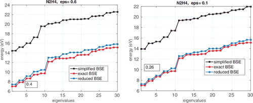
This effect can be also seen in Figure 2 for N₂H₄ molecule demonstrating the convergence γ_n → ω_n and λ_n → ω_n with respect to the increasing rank parameter determining the auxiliary problem (the size of the reduced basis set is m₀ = 30). The left and right figures correspond to the rank truncation thresholds, ϵ = 0.6 and ϵ = 0.1, respectively. The quantities λ_n, γ_n and ω_n are marked by black, blue and red colours, respectively.

Figure 2. Comparison of m₀ = 30 lower eigenvalues for the reduced and exact BSE systems vs. ϵ in the case of N₂H₄ molecule. The number in a text box indicates the error in the first eigenvalue |γ₁ − ω₁|.

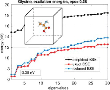
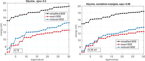
Figure 3 represents similar results for amino acid glycine, C₂H₅NO₂, with the BSE matrix size 6000 × 6000. In this case, the truncation thresholds ϵ = 0.2 leads to the rank parameters R_V = 54 , $R_{\bar{W}}=50$, $R_{\tilde{W}}=50$ and the error for the minimal eigenvalue, ω₁ = 0.72 eV. For ϵ = 0.08, we have the rank parameters R_V = 100 , $R_{\bar{W}}=215$, $R_{\tilde{W}}=129$ and the error for the minimal eigenvalue equals to 0.38 eV.

Figure 3. Comparison of m₀ = 30 lower eigenvalues for the reduced and exact BSE systems vs. ϵ in the case of Glycine amino acid The number in a text box indicates the error in the first eigenvalue |γ₁ − ω₁|.

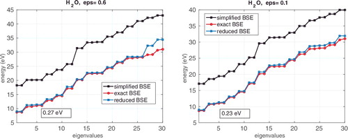
The lowest values of the BSE excitation energy for H₂O molecule computed by solving our exact system is 8.72 eV which agrees with the value 8.7 eV for ice water presented in [44]. The reduced basis method using the rank truncation threshold ϵ = 10⁻¹ provides the value 8.95 eV.

Figure 4, left and right, illustrates the BSE energy spectrum of the H₂O molecule for the lowest N_red = 30 eigenvalues vs. the rank truncation parameters ϵ = 0.6 and 0.1, where the ranks of V and the BSE matrix block $\tilde{W}$ are equal to 4, 5 and 28, 30, respectively, while the block $\bar{W}$ remains unchanged. For the choice ϵ = 0.6 and ϵ = 0.1, the error in the first (lowest) eigenvalue for the solution of the problem using the reduced basis is about 0.11 and 0.025 eV, respectively.

Figure 4. Comparison of m₀ = 30 lower eigenvalues for the reduced and exact BSE systems for H₂O molecule: ϵ = 0.6, left; ϵ = 0.1, right. The error in the first eigenvalue |γ₁ − ω₁| is shown in a text box.

Next, we present BSE calculations for chains of 16 and 32 hydrogen atoms placed in a 3D bounding box with the size 64³ bohr.³ The interatomic interval equals to 1.39 bohr. The HF calculations were performed with 64 and 128 Gaussian-type basis functions using grids of size 32, 768³ and 16, 384³, for computation of the core Hamiltonian and TEI, respectively. Cholesky factors of TEI matrix are of size 4096 × 175 and 16, 384 × 348 for the chains with 16 and 32 hydrogen atoms.

Table 4 demonstrates the decay of the error in the lowest eigenvalues |γ₁ − ω₁| with respect to the tolerance ϵ in the rank approximation of the BSE matrix for the chains of hydrogen atoms, H₁₆ (896 × 896) and H₃₂ (3584 × 3584), where the numbers in brackets specify the BSE matrix size. We observe linear scaling of the corresponding ranks of V,$\bar{W}$ and $\tilde{W}$ with respect to the size of the system as expected. Since the rank of $\bar{W}$ decays slowly, we studied the case, with fixed rank($\bar{W}$) = max {rank(V), rank$\tilde{W}\}$ (usually it coincides with rank(V)). The improved accuracy of the resulting spectrum is achieved even for rather large ϵ = 2 × 10⁻¹.

Table 4. Accuracy (in eV) for the first eigenvalue, |γ₁ − ω₁| vs. ϵ-rank for V, $\bar{W}$ and $\tilde{W}$ for chains of 16 and 32 hydrogen atoms.

	ϵ	4 × 10^−1	2 × 10^−1	10^−1	10^−2
H16	Ranks V,$\bar{W}$,$\tilde{W}$	16, 77, 1	30, 178, 3	43, 305, 19	70, 421, 65
	|γ1 − ω1|	0.2	0.15	5.4 × 10^−4	8 × 10^−4
	rank($\bar{W}$)=rank(V)	16, 16, 1	30, 30, 3	43, 43, 19	70, 70, 65
	|γ1 − ω1|	0.54	0.32	0.16	0.18
H32	Ranks V,$\bar{W}$,$\tilde{W}$	31, 159, 1	60, 391, 4	85, 757, 37	141, 1792, 132
	|γ1 − ω1|	0.15	0.13	6.2 × 10^−3	2.2 × 10^−3
	rank($\bar{W}$)=rank(V)	31, 31, 1	60, 60, 4	85, 85, 37	141, 141, 132
	|γ1 − ω1|	0.54	0.32	0.14	0.14

Table 5. The model error |μ₁ − ω₁| in TDA approximation for different molecules.

	H2O	H2O2	N2H4	C2H5OH	Glycine
err(eV)	0.083	0.13	0.06	0.064	0.045

4.2. Reduced basis approach to the Tamm–Dancoff model

It is interesting to apply the reduced basis approach described above to the so-called TDA [3], which corresponds to setting the matrix B = 0 in Equation (3.3(3.3) $$F\left(\begin{array}{c}{\mathbf{x}}_n\\ {\mathbf{y}}_n\end{array}\right)\equiv \left(\begin{array}{cc}\hfill A& \hfill B\\ \hfill B^{*}& \hfill A^{*}\end{array}\right)\left(\begin{array}{c}{\mathbf{x}}_n\\ {\mathbf{y}}_n\end{array}\right)={\omega }_n\left(\begin{array}{cc}\hfill I& \hfill 0\\ \hfill 0& \hfill -I\end{array}\right)\left(\begin{array}{c}{\mathbf{x}}_n\\ {\mathbf{y}}_n\end{array}\right),$$(3.3) ). It also allows to estimate the difference between the excitation energies from the full BSE model and those obtained by the TDA, which introduces an additional small model error.

The TDA model simplifies Equation (3.3(3.3) $$F\left(\begin{array}{c}{\mathbf{x}}_n\\ {\mathbf{y}}_n\end{array}\right)\equiv \left(\begin{array}{cc}\hfill A& \hfill B\\ \hfill B^{*}& \hfill A^{*}\end{array}\right)\left(\begin{array}{c}{\mathbf{x}}_n\\ {\mathbf{y}}_n\end{array}\right)={\omega }_n\left(\begin{array}{cc}\hfill I& \hfill 0\\ \hfill 0& \hfill -I\end{array}\right)\left(\begin{array}{c}{\mathbf{x}}_n\\ {\mathbf{y}}_n\end{array}\right),$$(3.3) ) to a standard Hermitian eigenvalue problem (4.1) $$A{\mathbf{x}}_n={\mu }_n{\mathbf{x}}_n,{\mathbf{x}}_n\in {\mathbb{R}}^{N_{ov}}A\in {\mathbb{R}}^{N_{ov}\times N_{ov}}$$(4.1) with the factor-two smaller matrix size N_ov. The reduced basis approach via low-rank approximation described in Section 3.2 can be applied directly to the TDA equation.

Below we present numerical tests indicating that the approximation error introduced by the TDA compared with the initial BSE system (3.3(3.3) $$F\left(\begin{array}{c}{\mathbf{x}}_n\\ {\mathbf{y}}_n\end{array}\right)\equiv \left(\begin{array}{cc}\hfill A& \hfill B\\ \hfill B^{*}& \hfill A^{*}\end{array}\right)\left(\begin{array}{c}{\mathbf{x}}_n\\ {\mathbf{y}}_n\end{array}\right)={\omega }_n\left(\begin{array}{cc}\hfill I& \hfill 0\\ \hfill 0& \hfill -I\end{array}\right)\left(\begin{array}{c}{\mathbf{x}}_n\\ {\mathbf{y}}_n\end{array}\right),$$(3.3) ) remains on the level of 0.003 Hartree for several compact molecules (see Table 5). This table indicates a tendency to decrease the TDA model error for larger molecules, say 0.0017 Hartree (0.045 eV) for glycine amino acid.

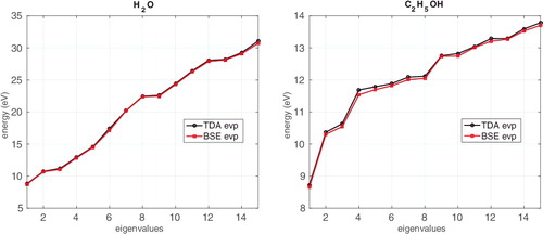
Figure 5 displays the error of TDA approximation in comparison with the full BSE system for the first m₀ = 15 lower eigenvalues on the examples of H₂O and C₂H₅OH molecules.

Figure 5. Comparison between m₀ = 15 lower eigenvalues μ_n and ω_n for the TDA and full BSE models, respectively, on the examples of H₂O and C₂H₅OH molecules.

5. Conclusions

This paper introduces and analyses the reduced basis method for computation of several lowest eigenvalues in the BSE, based on the solution of an auxiliary, simplified eigenvalue problem via diagonal plus low-rank approximations to the BSE matrix blocks. The reduced spectral problem of small size is derived via projection of the full BSE matrix onto the reduced basis set, composed of several dominant eigenvectors of the simplified problem. The ϵ-rank bounds for the requested subtensors of the TEI tensor represented in the basis set of HF MOs are proved in Lemmas 2.1 and 2.2. Asymptotic estimates on storage demands are provided. Numerical tests confirm merely quadratic error behaviour in the excitation energies with respect to the accuracy of the rank approximation. The particular construction of the BSE matrix is based on the BSE-GW approximation with non-interacting HF Green's function (we follow the construction considered in [14]).

The main goal of the present paper is the development and numerical verification of the reduced basis method applied to large-scale BSE eigenvalue problems. Potential efficiency of the approach is illustrated numerically on the examples of single molecules and finite hydrogen chains. The numerical studies demonstrate that eigenvalues of the reduced spectral problem provide a sufficient approximation to the lowest excitation energies of the exact BSE system. For all the examples considered so far, the accuracy of the order of 0.15 − 0.3 eV was achieved³by the reduced basis method with rather moderate ranks as indicated in Tables 3 and 4. The behaviour of the approximation error vs. rank parameters remains similar for compact molecules and for finite chains of atoms.

Future work will be focused on application and development of efficient linear algebra algorithms for fast and accurate solution of the arising large eigenvalue problems taking into account data-sparse block structures. In particular, the complementary structural representations to the matrix $\bar{W}$ may enhance the accuracy of the reduced basis method. These issues will be considered in a forthcoming paper.

Another possible research direction is concerned with the quantised tensor train (QTT) approximation [45] of the long vectors and large matrices involved, in order to perform the fast matrix–vector calculations in the QTT tensor arithmetics with ϵ-rank truncation, see [46].

Acknowledgments

The authors would like to thank A. Savin (UPMC, Paris) and J. Toulouse (UPMC, Paris) for valuable comments on the problem setting for the BSE model and for providing useful references. Furthermore, we acknowledge helpful remarks by C. Yang (LBL, Berkeley) on the initial draft of the manuscript.

Disclosure statement

No potential conflict of interest was reported by the authors.

Notes

* Dedicated to Prof. Andreas Savin on occasion of his 65th birthday.

1. In [14], it was demonstrated that in the case of small interatomic distance this model remains in a good agreement with the reference data for full configuration–interaction calculations though it does not describe the dissociation case. The BSE model was shown to provide satisfactory results in the latter case when using the exact Green's function.

2. Though one can notice that the static-screened interaction matrix, responsible for the exchange interaction of electrons, does not allow the high-accuracy low-rank approximation, as it is already known about the HF exchange.

3. For example, paper [11] assumes the BSE model errors in the range of 0.1–0.3 eV as the acceptable precision.

References

- E. Runge and E. Gross, Phys. Rev. Lett. 52 (12), 997–1000 (1984).
- E. Gross and W. Kohn, Adv. Quantum Chem. 21 (255), 287–323 (1990).
- M.E. Casida, in Recent Advances in Density Functional Methods, Part I, edited by D.P. Chong (World Scientific, Singapore, 1995), Vol. 155, pp. 1207–1216.
- R.E. Stratmann, G.E. Scuseria, and M.J. Frisch, J. Chem. Phys. 109, 8218 (1998).
- C. Cramer and D. Truhlar, Phys. Chem. Chem. Phys. 11 (46), 10757–10816 (2009).
- L. Reining, V. Olevano, A. Rubio, and G. Onida, Phys. Rev. Lett. 88, 066404 (2002).
- E.E. Salpeter and H.A. Bethe, Phys. Rev. 82 (2), 309–310 (1951).
- L. Hedin, Phys. Rev. 139, A796 (1965).
- G. Onida, L. Reining, and A. Rubio, Rev. Mod. Phys. 74, 601 (2002).
- W.G. Schmidt, S. Glutsch, P.H. Hahn, and F. Bechstedt, Phys. Rev. B 67, 085307 (2003).
- S. Körbel, P. Boulanger, I. Duchemin, X. Blase, M. AL Marques, and S. Botti, J. Chem. Theory Comput. 10 (9), 3934–3943 (2014).
- E. Rebolini, J. Toulouse, A.M. Teale, T. Helgaker, and A. Savin, Phys. Rev. A 91, 032519 (2015).
- J. Deslippe, G. Samsonidze, D.A. Strubbe, M. Jain, M.L. Cohen, and S. Louie, Comp. Phys. Commun. 183, 1269 (2012).
- E. Rebolini, J. Toulouse, and A. Savin, in Concepts and Methods in Modern Theoretical Chemistry, edited by S. Ghosh and P. Chattaraj, Vol 1, Electronic Structure and Reactivity, (CPC Press, Boca Raton, 2013), p. 367.
- E. Rebolini, J. Toulouse, and A. Savin, Mol. Phys. 111, 1219 (2013).
- V. Khoromskaia, Comp. Methods Appl. Math. 14, 89 (2014).
- V. Khoromskaia and B.N. Khoromskij, Comp. Phys. Commun. 185 (1), 2–10 (2014).
- B. N. Khoromskij, Chemometr. Intell. Lab. Syst. 110 (1), 1–19 (2012).
- V. Khoromskaia and B.N. Khoromskij, Phys. Chem. Chem. Phys. 17, 31491 (2015).
- V. Khoromskaia, B.N. Khoromskij, and R. Schneider, SIAM J. Sci. Comput. 35 (2), A987–A1010 (2013).
- P. Benner and H. Faßbender, Linear Algebra Appl. 263, 75 (1997).
- P. Benner, V. Mehrmann, and H. Xu, Numer. Math. 78 (3), 329–358 (1998).
- D. Kressner, Numerical Methods for General and Structured Eigenvalue Problems, Vol. 46, Lecture Notes in Computational Science and Engineering (Springer, Berlin/Heidelberg, 2005).
- H. Faßbender and D. Kressner, GAMM Mitteilungen 29 (2), 297–318 (2006).
- M. Shao, F.H. da Jornada, C. Yang, J. Deslippe, and S. Louie, Linear Algebra Appl. 488, 148 (2016).
- A. Bunse-Gerstner and H. Faßbender, in Numerical Algebra, Matrix Theory, Differential-Algebraic Equations and Control Theory, edited by P. Benner, M. Bollhöfer, D. Kressner, C. Mehl, and T. Stykel (Springer International Publishing, Heidelberg, 2015), pp. 3–23.
- Z. Bai and R.-C. Li, SIAM J. Matrix Anal. Appl. 33 (4), 10751100 (2012).
- Z. Bai and R.-C. Li, SIAM J. Matrix Anal. Appl. 34 (2), 392–416 (2013).
- A. Bunse-Gerstner, R. Byers, and V. Mehrmann, SIAM J. Matrix Anal. Appl. 13 (2), 419–453 (1992).
- D. Mackey, N. Mackey, and F. Tisseur, Electron. J. Linear Algebra 10, 106 (2003).
- D. Mackey, N. Mackey, C. Mehl, and V. Mehrmann, SIAM J. Matrix Anal. Appl. 28 (4), 1029–1051 (2006).
- C. Mehl, SIAM J. Matrix Anal. Appl. 30, 291 (2008).
- P. Benner, H. Faßbender, and C. Yang, Some remarks on the complex J-symmetric eigenproblem. Max Planck Institute Magdeburg, Preprint MPIMD/15-12 (July 2015).
- E. Napoli, E. Polizzi, and Y.Y. Saad, Efficient estimation of eigenvalue counts in an interval. arXiv:1308.4275v2, 2014.
- L. Lin, Y. Saad, and C. Yang, Approximating spectral densities of large matrices. arXiv:1308.5467.v2., 2015.
- P. Benner, V. Mehrmann, and D. Sorensen, editors, Dimension Reduction of Large-Scale Systems, Vol. 45, Lecture Notes in Computational Science and Engineering (Springer, Berlin, 2005).
- S. Reine, T. Helgaker, and R. Lindh, WIREs Comput. Mol. Sci. 2 (2), 290–303 (2012).
- T. Helgaker, P. Jørgensen, and J. Olsen, Molecular Electronic-Structure Theory (Wiley, Chichester, 1999).
- N. Beebe and J. Linderberg, Int. J. Quantum Chem. 12 (4), 683–705 (1977).
- S. Wilson, Comput. Phys. Commun. 58, 71 (1990).
- N. Higham, in Reliable Numerical Computations, edited by M.G. Cox and S.J. Hammarling (Oxford University Press, Oxford, 1990), pp. 161–185.
- T.H.J. Dunning, J. Chem. Phys. 90, 1007 (1989).
- H.-J. Werner, P.J. Knowles, G. Knizia, F.R. Manby, and M. Schütz, Wiley Interdiscip. Rev. Comput. Mol. Sci. 2 (2), 242–253 (2011).
- A. Hermann, W.G. Schmidt, and P. Schwerdfeger, Phys. Rev. Lett. 100, 207403 (2008).
- B.N. Khoromskij, J. Constr. Approx. 34 (2), 257–289 (2011).
- S. Dolgov, B. Khoromskij, D. Savostyanov, and I. Oseledets, Comp. Phys. Commun. 185 (4), 1207–1216 (2014).