Development of intermolecular potential models for electrolyte solutions using an electrolyte SAFT-VR Mie equation of state

ABSTRACT

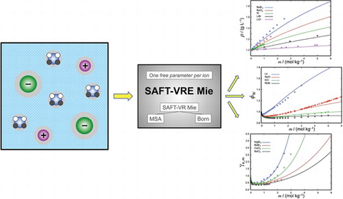
We present a theoretical framework and parameterisation of intermolecular potentials for aqueous electrolyte solutions using the statistical associating fluid theory based on the Mie interaction potential (SAFT-VR Mie), coupled with the primitive, non-restricted mean-spherical approximation (MSA) for electrolytes. In common with other SAFT approaches, water is modelled as a spherical molecule with four off-centre association sites to represent the hydrogen-bonding interactions; the repulsive and dispersive interactions between the molecular cores are represented with a potential of the Mie (generalised Lennard-Jones) form. The ionic species are modelled as fully dissociated, and each ion is treated as spherical: Coulombic ion–ion interactions are included at the centre of a Mie core; the ion–water interactions are also modelled with a Mie potential without an explicit treatment of ion–dipole interaction. A Born contribution to the Helmholtz free energy of the system is included to account for the process of charging the ions in the aqueous dielectric medium. The parameterisation of the ion potential models is simplified by representing the ion–ion dispersive interaction energies with a modified version of the London theory for the unlike attractions. By combining the Shannon estimates of the size of the ionic species with the Born cavity size reported by Rashin and Honig, the parameterisation of the model is reduced to the determination of a single ion–solvent attractive interaction parameter. The resulting SAFT-VRE Mie parameter sets allow one to accurately reproduce the densities, vapour pressures, and osmotic coefficients for a broad variety of aqueous electrolyte solutions; the activity coefficients of the ions, which are not used in the parameterisation of the models, are also found to be in good agreement with the experimental data. The models are shown to be reliable beyond the molality range considered during parameter estimation. The inclusion of the Born free-energy contribution, together with appropriate estimates for the size of the ionic cavity, allows for accurate predictions of the Gibbs free energy of solvation of the ionic species considered. The solubility limits are also predicted for a number of salts; in cases where reliable reference data are available the predictions are in good agreement with experiment.

KEYWORDS:

• Electrolytes
• equation of state
• parameter estimation
• SAFT
• phase equilibrium

1. Introduction

Aqueous electrolyte solutions are liquid mixtures containing charged species, typically stemming from the dissociation equilibrium of the constituent ions of salts in water. The ubiquitous nature of electrolytes makes them relevant in many scientific and industrial applications. Examples of applications requiring a thermodynamic description of electrolyte solutions include the sequestration of carbon dioxide, the clean-up of process chemicals from nuclear waste, hydrate formation, scaling in pipelines, advanced process chemistry, corrosion processes, and flue-gas cleaning. Electrolyte solutions are also prevalent in geochemical and biological environments and the development of molecular models to describe their properties remains of great interest.

The presence of charged species (ionic components) in solution drastically alters the bulk thermodynamic properties of the mixture, usually leading to a lowering of the vapour pressure (with a corresponding increase in the boiling temperature), an increase in density, and changes in the viscosity and surface tension of the system. The theoretical description of thermodynamic properties of electrolyte solutions has proved a challenging task, and the body of work in this area has been less extensive than for non-electrolyte systems. The development of a successful theory of electrolyte solutions relies on both the availability of accurate inter-particle potentials for all of the species in the system and the ability to resolve the statistical–mechanical relations that lead to the bulk properties of interest. Much of the difficulty can be ascribed to the range of the electrostatic forces, and the corresponding paucity of analytic theories that can be used to describe the relevant many-body effects. Available theories predominantly incorporate the Coulombic nature of the ionic interactions with a much simplified representation of the neutral solvent molecules, which are often polar and, as in the case of water, can exhibit hydrogen-bonding interactions. The intricacy of the solvent–solvent, solvent–solute and solute–solute interactions and their corresponding interplay makes this a challenging area of research.

A so-called primitive formulation is proposed in the classical approach of Debye and Hückel (DH) [1], whereby the solvent is represented as a continuum dielectric medium and the Poisson–Boltzmann equation [2,3] is solved in linear form. Waisman and Lebowitz [4] and Blum and Hoye [5,6] later solved an equivalent primitive model using integral equation theory within the mean-spherical approximation (MSA). A formulation of the MSA allowing for an explicit representation of the solvent was then developed by Wei and Blum [7], among others. In the late 1990s, molecular-based equations of state (EOSs), specifically the statistical associating fluid theory (SAFT) [8,9] and the cubic plus association (CPA) EOS [10], were combined with the classical approaches for charged species [1,5,6] and shown to provide an accurate description of the properties of strong electrolyte solutions [11–13], extending the range of applicability to more-concentrated solutions. The increasing accuracy in the description of the properties of the solvent and fidelity of the representation of the solvent–ion interactions has been exploited in subsequent work [14–22].

For applications where the partitioning of the charged species in different phases is of interest, further consideration of the electrostatic contribution that arises from the interactions of the ionic species with the medium is required. In the case of non-primitive models, where the polarity of the solvent is treated explicitly by including dipolar interactions, such a contribution arises naturally [23,24]. The solvent is treated explicitly only in terms of its non-electrostatic nature for most studies with the SAFT or cubic EOS electrolyte framework and, as a consequence, an additional contribution is necessary for an accurate representation of the thermodynamics (in particular, the chemical potential) of the ionic species due to the dielectric nature of the real medium. A simple treatment to account for the introduction of a charged species in a dielectric medium was provided by Born [25]. The Born contribution has now been incorporated within cubic and CPA EOSs [26,27], and, more recently, within the ePPC-SAFT [20] and SAFT-VRE [21] approaches. A non-primitive treatment that incorporates a polar solvent within a SAFT formalism has also been presented [17,28–30]. These studies highlight the importance of accurately predicting the dielectric constant of the system, as well as the impact of taking into account ion-pairing phenomena. The work of Maribo-Mogensen and co-workers [22,31,32] is also particularly relevant in this context, where the focus is on improving the description of the static permitivity, a key property of electrolyte solutions and which is commonly incorporated empirically from a knowledge of the experimental value.

The SAFT-VRE [13] approach has recently been revised [21] to acknowledge the specific importance of incorporating the Born [25] contribution to the free energy of the system, thus accounting for the charging process of the ionic species in the solvent medium. A robust set of models for strong electrolytes was presented, providing an accurate description of a broad range of properties, including the Gibbs free energy of solvation, with the aid of the Born treatment. The model and theory proposed in [21] are based on an underlying square–well interaction potential following the original SAFT-VR framework [33,34]. The SAFT-VR EOS has now been reformulated for the more versatile and realistic Mie [35] potential form together with an improvement in the underlying statistical–mechanical theory, now taken to third order in the high-temperature perturbation expansion [36]. The novel SAFT-VR Mie EOS has brought a new level of reliability in the development of an accurate platform for the thermodynamic properties of complex fluids and fluid mixtures [36–38]. The approach has also been cast as a group-contribution methodology (SAFT-γ) [39,40], where the molecules are represented in terms of the underlying chemical functional groups, providing an enhanced predictive capability. Importantly, the improved theoretical framework provides models that reflect more accurately the physics of the systems they describe, reducing the reliance on re-adjusting the values of the intermolecular parameters to capture given thermodynamic properties of interest (although, of course, the estimation of the key parameters is still necessary). These advances have not yet been extended to include a description of electrolyte solutions. The purpose of our current work is to redress this: as will be shown, the introduction of a more rigourous physical description in the resulting SAFT-VRE Mie EOS allows for a reduction in the number of adjustable parameters, as compared with the previous SAFT-VRE formulation [21]. In addition, we develop electrolyte model parameters to represent the thermodynamic properties of a broad range of aqueous solutions of strong electrolytes including monovalent and divalent ions, and assess the performance of the models by making appropriate comparisons with available experimental data.

Our paper is set out as follows: in the following section, we describe the underlying SAFT-VRE Mie theory; in Section 3, the technique for the development of our model intermolecular parameters is discussed in detail; in Section 4, we present the models developed, which comprise group-I metal cations, from lithium to rubidium, selected group-II (divalent) metallic cations, the hydronium cation, the halide anions from fluoride to iodide, and the hydroxide anion; our models and theory are applied in Section 5 for the description of thermodynamic properties, including the mean-ionic activity coefficients, the osmotic coefficients, the vapour pressure, the density, and the solvation energies of the ions for aqueous solutions containing these species; we present our conclusions in Section 6.

2. Methodology

2.1. Thermodynamic system

At a specified temperature and total volume, we consider fluid mixtures consisting of water (the solvent) and a salt which is fully dissociated into its constituent ions following an equilibrium reaction. For a salt MX, the equilibrium can be described as (1) where the salt dissociates into the metal ion M of valency Z₊ and the counterion X of valency Z₋ in the stoichiometry ν₊: ν₋. The dissociation reaction is fully shifted towards the products, i.e. no neutral salt is present in the mixture. Here we consider only the dissociated ions present in the solvent as solutes.

2.2. SAFT-VRE Mie Helmholtz free energy

In broad strokes, the theory as outlined in the present paper follows the approach developed in previous work [21], as applied to the SAFT-VR Mie formalism [36] in conjunction with the Wertheim [41–46] TPT1 treatment of the association in water [37] (based on the Lennard-Jones form of the association kernel). We refer to the resulting theory as SAFT-VRE Mie. A short overview of the main expressions is given here for completeness; for further details, the reader is referred to the original publications.

The Helmholtz free energy A of the system is written as a sum of terms, arising from a perturbation approach, each of which corresponds to a specific physical contribution in addition to the usual ideal contribution represented as A^ideal: (2) where the non-electrostatic and electrostatic contributions are treated separately. The residual non-electrostatic terms A^monomer, A^chain, and A^association describe the common SAFT contributions: the effect of introducing monomeric spherical segments interacting through Mie potentials; the effect of bonding the monomeric spherical segments into molecular chains; and the effect of molecular association through short-ranged directional forces, such as those arising in hydrogen bonding. Collectively, these terms correspond to the non-electrolyte SAFT-VR Mie EOS [36]. The electrostatic terms comprise A^ion and A^Born, both represented within the primitive model formalism, where the solvent is described by a dielectric medium (it is important to note, however, that the solvent is treated explicitly in the non-electrostatic part of the free energy). The change in free energy associated with the process of charging the ions in the solvent is incorporated in A^Born following the Born [25] model, and the effect of electrostatic interactions between charged species is described with A^ion using the primitive non-restricted MSA [5,6] model.

2.2.1. Non-electrostatic contributions

The non-electrostatic contributions are modelled following the SAFT-VR Mie EOS [36], in place of the SAFT-VR SW EOS applied in previous work [21]. In the SAFT-VR Mie formalism, molecules are modelled as chains comprising m_seg bonded spherical segments of diameter σ, interacting through a spherically symmetric Mie potential [35,36] characterised by a repulsive exponent λ_r, an attractive exponent λ_a, and a dispersive interaction energy ϵ. The Mie pair potential for the interaction between two unlike spherical segments labelled i and j can be expressed as (3) where r_ij is the distance between the centres of segments i and j. Additional off-centre, short-ranged square–well potential sites can be assigned to segments of particular species to mediate hydrogen-bonding associative interactions.

The ideal Helmholtz free-energy term of the mixture is given by [47] (4) where k_B is the Boltzmann constant, N is the number of molecules, n_c is the number of species (recalling that in our work, we assume the salts to be fully dissociated so that the anion and cation are treated as separate species), ρ_i = N_i/V is the number density of component i at volume V, where N_i is the number of molecules of component i, x_i = N_i/N is the mole fraction of component i, and Λ³_i is the de Broglie volume for component i which includes all the relevant translational, vibrational and rotational contributions to the kinetic energy.

The monomer contribution of the Helmholtz free energy for the mixture of spherical segments interacting via Mie potentials is obtained as a third-order perturbation expansion following the high-temperature perturbation scheme of Barker and Henderson [36,48]: (5) where the reference hard-sphere term A_HS is represented with the expression of Boublík and Mansoori [49,50] for mixtures of hard spheres. An analytical expression for the first-order mean-attractive energy A₁ is obtained through the use of the mean value theorem and a mapping of packing fractions, following the original SAFT-VR [33] approach, as applied for Mie fluids within a range of exponents of 5 ≤ λ ≤ 100 [36]. The second-order fluctuation term A₂ is calculated using the improved macroscopic compressibility approximation (MCA) of Zhang [51] with the modification proposed by Paricaud [52]. An empirical expression is used for the third-order perturbation term A₃, with coefficients obtained to reproduce the critical point and fluid-phase equilibrium of Mie fluids [36].

Although not relevant in the case of the molecules considered in our current work, for completeness and to provide a general framework, it is useful to mention briefly the contribution to the free energy due to the formation of chains of bonded Mie segments. This contribution, as in other SAFT approaches, is obtained through the TPT1 formalism of Wertheim [46,53], which is expressed in terms of the radial distribution function (RDF) of the monomer fluid, evaluated at contact distance of the segments. In the case of a mixture, the expression is given as (6) where is the RDF of the monomeric Mie fluid system at contact σ_ii. Note that in our current work, the number of segments per chain is m_{seg, i} = 1 for all of the species i considered and, as a result, A^chain is equal to zero.

The association contribution of the Helmholtz free energy is also derived from the formalism presented by Wertheim [41,42], which can be written as [45,46] (7) for the case of a mixture of n_c species, and where the second summation is over the types of sites of species i; n_{sites, i} is the number of site types on a molecule and n_{a, i} is the number of sites of type a on component i. The variable X_{a, i} represents the fraction of molecules not bonded at a given site type a on species i and is obtained as the solution of a set of mass action equations for each bonding interaction: (8) In this expression, indices i and j represent the components, indices a and b represent the sites, and Δ_ab,ij is the integrated association strength between site type a on molecule i and site type b on molecule j. The integrated association strength can be expressed [37] as a product of the association kernel I, the Mayer function F_ab of the bonding interaction of strength ϵ^HB_{ab, ij}, and the bonding volume K_ab: (9) The association kernel I has been parameterised as a polynomial in the dimensionless temperature T^* = k_BT/ϵ, dimensionless density ρ^* = Nσ³/V, and the repulsive exponent λ_r, as reported in [37,38]; note that in our current work, we employ the Lennard-Jones (12-6) form of the association kernel.

2.2.2. Electrostatic contributions

The Coulombic interactions pertaining to the charged species are represented following an unrestricted primitive model where each of the ionic species is considered to be spherical with a central point charge; the diameters of the ions are not restricted to be all identical. In this approach, the explicit representation of the polarity of the solvent molecules is replaced by a dielectric medium, of relative static permittivity D. Such a treatment of the solvent simplifies the inherently complex model for the Coulomb potential of the charged ions [54], while retaining the main feature of electrolytes. The other ion–ion and ion–solvent non-electrostatic interactions (repulsion, dispersion and, if needed, hydrogen bonding) of the ionic species are taken into account using the SAFT-VR Mie expressions as outlined in Section 2.2.1.

The change in the free energy due to the insertion of all of the ions in the dielectric medium is accounted for by the free energy of solvation. In our work, the process of solvation is described with the Born approach [25] which, though simplistic, captures the basic thermodynamic features. In the Born model, a spherical cavity is created, of a size suitable for each of the individual ions. A point charge of magnitude and sign commensurate with that particular ion is then embedded, and an expression for the free-energy change associated with this process is obtained through the Born cycle, which is illustrated in Figure 1: the system is first discharged to represent a corresponding system of non-interacting hard spheres in a vacuum; the dielectric medium is then switched on; finally, a non-interactive recharging of the ions is carried out. The premise of the Born model is that a spherical cavity of diameter is created in the dielectric medium for each ion i, independent of any others, leading to the following contribution to the Helmholtz free energy: (10) Here, the index i runs over all n_ion charged species, e = 1.602 × 10⁻¹⁹ C is the elementary charge, ε₀ = 8.854 × 10⁻¹² C² J⁻¹m⁻¹ is the static permittivity of the medium in vacuum, D is the relative static permittivity of the medium, and Z_i is the valency of ion i.

Figure 1. Schematic representation of the Born cycle. (1) The system consists of hard spheres and non-interacting charged hard spheres in vacuum; (2) the charged hard spheres are discharged in vacuum; (3) the system consists of (uncharged) hard spheres in a dielectric medium represented by the dotted background; (4) the system consists of hard spheres and non-interacting charged hard spheres in a dielectric medium.

A particular challenge of implementing the Born model is the interpretation and parameterisation of the cavity diameter. The primitive model, in which the Born model is expressed, does not represent a convenient 1:1 mapping to the intermolecular potential parameters utilised in the explicit solvent representation of the system. It is common, however, to take the cavity diameter of the Born model as that represented by the diameter σ_ii of the intermolecular potential of the ion itself.

Ion–ion interactions are represented with the Coulomb potential in a dielectric medium, i.e. (11) where r_ij is the centre–centre distance between charges i and j. In the case of the primitive model, one of two classical theories is typically used to resolve the corresponding residual free energy: either the Debye–Hückel theory [1] or the mean spherical approximation (MSA) [6,55]. As shown by Maribo-Mogensen et al. [56], both approaches lead to a similar representation of the macroscopic thermodynamic properties of electrolyte solutions; the material difference between the two is the parametrisation procedure for the corresponding models. In our current paper, the MSA theory is applied following the formulation of Blum [5,6], as laid out in previous work [21]. The change in the Helmholtz free energy due to the electrostatic interactions between charged species within the MSA formalism can be expressed as (12) Here, U^MSA is the MSA contribution to the internal energy U, and Γ is the screening length of the electrostatic forces. The MSA internal energy is given by (13) Δ represents the packing fraction of the ions as a function of their diameter σ_ii: (14) The functions P_n and Ω are coupling parameters, where P_n couples to the charge of the ions, whereas Ω relates to the packing fraction of the ions. Both are functions of the ionic parameters, as well as the screening length of the ions: (15) (16) Finally, the screening length Γ is a function of the relative static permittivity and the effective charge Q_i(Γ) of the ions, leading to an implicit formulation through Q_i: (17) where the effective charge is related to the electric charge of the individual species and the P_n coupling parameter: (18)

The implicit nature of the MSA formulation requires an iterative procedure to establish Γ. In the present implementation, a successive substitution procedure is followed with an initial guess, Γ₀, for the screening length obtained from the Debye–Hückel estimate for the screening length, (19) where κ is the inverse Debye–Hückel length. The addition of the Born term and the MSA term to the SAFT-VR Mie theory, detailed in Section 2.2.1, constitutes the SAFT-VRE Mie theory developed in our current work.

2.2.3. Auxiliary model: the relative static permittivity

The relative static permittivity D is calculated with a Harvey–Prausnitz model [57] as outlined in a previous paper [21]. This correlative model depends on the solvent composition, density, and temperature, and thereby exhibits an implicit dependence on the ion concentration. The value of D in the case of a pure solvent j is characterised by a volume parameter d_V,j and by a temperature parameter d_T,J. A combined static permittivity parameter d_j is calculated for a given temperature following the relation (20) The relative static permittivity is then obtained as (21) where ρ_j = N_j/V is the number density of the solvent.

2.3. Thermodynamic properties of electrolyte solutions

The concentration of a given salt MX is often quantified in terms of the molality, denoted here by m_MX, and defined as the molar amount (mol) of salt per kilogram of solvent j. The mole fraction of a given ion i can be calculated from the molality as (22) where ν_i is the stoichiometric coefficient of ion , and MW_j denotes the molecular weight of the solvent in units of kg mol⁻¹.

In addition to the common thermodynamic properties of equilibrium fluids, the activity coefficients γ_i of the ions and the osmotic coefficient Φ of the solution are key properties often reported for electrolyte solutions. The generic activity coefficient of component i, denoted here by γ_{i, x}, is related to the chemical potential μ_i of component i through the following expression: (23) the product c_iγ_{i, x} yields the activity a_i of component i. In Equation (23(23) ), is a reference term, N is the composition vector, c_i is a measure of concentration, and the subscript x denotes that γ_{i, x} is expressed in units commensurate with those of c_i. Depending on the nature of the system in question, it may however be convenient to express the activity coefficient in one of a variety of ways. For the standard symmetrical activity coefficient, the concentration is measured in terms of the mole fraction x_i of component i: (24) where the reference term is identical to that of the chemical potential of pure component i at the system temperature and pressure, i.e. , and the activity can be calculated as a_i(T, p, N) = x_iγ_{i, x}(T, p, N). As ions cannot be related meaningfully to the pure system, the appropriate reference for the activity coefficients is the rational asymmetric scale, for which the activity coefficient of ion i, γ_{i, *}, has a value of one in the limit of infinite dilution of ion i. In practice, the calculation of γ_{i, *} is carried out through the fugacity coefficient ϕ_i: (25) where N* is the composition vector at infinite dilution of ion i.

The fugacity coefficient is obtained from the residual chemical potential μ^Res = μ − μ^ideal, taking into account the ideal state conversion for properties expressed at a given pressure, obtained from an EOS expressed with volume as the independent variable. In this case, the fugacity coefficient is obtained as (26) Here, V_p denotes the volume corresponding to the specified pressure and Z = pV_p/(Nk_BT) denotes the thermodynamic compressibility factor.

It is the usual convention to report properties of ions in terms of the molality, whereby the activity coefficients are presented in the molal-based scale, γ_{i, m}. This scale employs a convention of a hypothetical ideal solution at unit molality such that ∑_im_i → 0 ⇒ γ_{i, m} → 1. The conversion between the rational asymmetric scale and the molal-based scale follows as [58] (27) with a corresponding change in the reference term utilised in the calculation of the chemical potential based on γ_{i, m}, and where x_j denotes the mole fraction of the solvent.

The electrolytic properties of the solution can be collated in the mean ionic activity coefficient (MIAC), γ_{±, m}, calculated as an average of cationic and anionic contributions: (28) The contribution of the solvent j to the thermodynamics of the system can be characterised through the osmotic coefficient Φ. The osmotic coefficient provides a convenient re-scaling of the activity of the solvent, in order to accentuate its variation at low solute concentrations: (29) The properties of solutes and solvents are not independent, and must fulfil the Gibbs–Duhem relation [59]. The MIAC and the osmotic coefficient Φ are related through the following relationship: (30)

Finally, Φ and γ_{±, m} can be related to the change in the Gibbs energy of solvation ΔG_{solv, i} of ion i through the fugacity coefficient: (31) where ϕ_i is the fugacity coefficient of component i at infinite dilution in solvent j, p_ref is the pressure of the reference state for the change in the Gibbs free energy, and m° is the standard state molality of 1 mol kg^{− 1}.

2.4. Phase equilibrium

The conditions which enforce phase equilibrium of electrolyte solutions are similar to those of non-electrolyte systems, with additional constraints related to the charge balances and the necessary charge neutrality of a given phase. First, the thermal and mechanical equilibrium conditions must be satisfied, i.e. (32) (33) Here, the index N_phases accounts for all of the phases, denoted as superscript Greek letters. In addition, a relationship in each equilibrium phase is required for the chemical potentials of each species in the mixture. As a consequence of treating electrolyte solutes as fully ionised in solution, the additional constraints required to characterise phase equilibrium will depend on the nature of the phases considered.

2.4.1. Fluid-phase equilibria

In the consideration of equilibrium between two (or more) fluid phases, equality of chemical potentials is required for each neutral species. Here it is assumed the solvent is pure and the only neutral species present so that: (34) while for each pair of charged species i and i′, a constant relative difference of chemical potentials across electro-neutral phases is satisfied [60]: (35) (36)

The solution to the equilibrium conditions is obtained with a Levenberg–Marquardt [61,62] algorithm, allowing for the presence of salts in all fluid phases, including the gas phase. The volume dependence of the relative static permittivity and the inclusion of the Born free energy term in the underlying theory deliver a model where the ions naturally partition predominantly into the denser liquid phase, with only trace amounts in the gaseous phase, in agreement with experimental observation.

2.4.2. Solid–liquid phase equilibria

The description of phase equilibrium between solid and liquid phases containing electrolytes is linked to the chemical equilibrium governing the dissociation of the solvated electrolyte leading to the formation of charged species in solution. The solid phase consists of the pure unsolvated crystalline salt MX in equilibrium with a liquid phase saturated in salt. Assuming complete dissociation of the dissolved salt, the phase and chemical equilibria require that the chemical potential of the crystalline salt in the solid phase is equal to the sum of the chemical potentials of the solvated ions , with i =M,X: (37) where M represents the cation and X the anion. The molal composition vector of the saturated aqueous phase is represented by m^sat, and the molality of solvated ion i is related to the salt molality through (38) where m_MX^sat is the solubility limit of salt MX.

The chemical potential of the solid salt is obtained from (39) where μ⁰_MX is the reference chemical potential of the pure solid salt and a_MX is the activity of the pure salt, taken to be unity; the reference chemical potential of a pure compound is also its molar Gibbs free energy of formation .

The chemical potential of solvated ion i is expressed on a molality basis as (40) where the reference chemical potential μ°_i(T, p, m°) of ion i refers to a hypothetical ideal solution of unit molality (m^○ = 1 mol kg⁻¹), and γ_{i, m} is the molal-based activity coefficient given by Equation (27(27) ). The chemical potential of ion i at the reference state of unit molality corresponds to the molar Gibbs free energy of formation of 1 mol kg⁻¹ of the solvated ion.

Using Equation (38(38) ) and the expressions for the chemical potential of the solid salt and solvated ions, the solid–liquid equilibrium condition for fully dissociated salts given by Equation (37(37) ) can be rewritten to obtain a solubility equation for the salt as (41) In this expression, K_sp is the solubility product of the salt given by (42)

3. Model development

We consider aqueous solutions of strong electrolytes focusing particularly on the halide salts of alkali metals and alkaline earth metals, as well as aqueous strong acids and bases. These solutions are modelled as ternary mixtures composed of water, anions, and cations, under the assumption of a fully dissociated solute. The electrolyte solutes are therefore modelled via the constituent monovalent and divalent atomic ions in the case of salts, while molecular ions are also considered for the acid and base solutions.

In our current work, the ions are modelled as spherical, consisting of a single segment m_seg, i = 1) of diameter σ_ii, and carrying a single point charge q_i = Z_ie. All ions experience dispersion interactions, represented with Mie potentials of variable range, both with the solvent and with the other ions. A full description of the intermolecular potential requires the like energetic parameters as well as the cross-interaction parameters. The like parameters include the diameter σ_ii, the interaction energy ϵ_ii, and the repulsive and attractive exponents of the Mie potential, λ_r,ii and λ_a,ii, respectively. Similarly, the cross-interaction parameters include the unlike diameter σ_ij, the unlike interaction energy ϵ_ij, and the corresponding repulsive and attractive Mie exponents, λ_r,ij and λ_a,ij.

We also consider associating molecular ions which interact with the solvent via hydrogen bonding, and which are therefore characterised by additional association parameters: the number of sites of type a on ion i (n_{a, i}), the unlike bonding energy ϵ^HB_{ab, ij}, and the corresponding bonding volume K_ab,ij between site a on ion i and site b on solvent j. For the development of molecular ions, we propose that the model of the molecular ion should be physically consistent with the model of the smallest neutral parent molecule giving rise to the ion. The SAFT-VR Mie model of the neutral parent molecule is used as a reference for the molecular ion and consequently the parameters of the two species, including the association parameters, will be related.

The parameterisation of the intermolecular potentials for the solvent and solute species dictate the fidelity of the proposed model. However, the complexity of our model demands the determination of a significant number of parameters, both for pure species and for unlike binary interactions. This results in a large parameter space which is known to be degenerate, yielding significant variability in the description of individual species. For charged species, the model development of electrolytes with equations of state is further complicated by the underlying premise that the ionic species can only be assessed in solution. In order to simplify the parameter estimation problem, we seek to limit the number of free parameters by assigning reasonable estimates to those parameters for which it is possible to use physical relationships to determine their value in the model. In our work, depending on the type of species i and j, the cross-interaction parameters are obtained either via combining rules or by parameter estimation, while pure-component parameters are assigned a priori values whenever possible.

3.1. Solvent model and static permittivity

We consider only aqueous electrolyte solutions and treat the solvent using the Mie model for water based on the Lennard-Jones association kernel developed in earlier work [37,40]. In this model, the water molecule comprises a single segment with four off-centre association sites, two of which are of the hydrogen type ‘H’ (n_H, j = 2) and two of the electron lone-pair type ‘e’ (n_e, j = 2), which mediate hydrogen bonding interactions. For completeness, the molecular potential parameters for this model of water are given in Table 1, together with the parameters required for the correlation of the dielectric constant (cf. Section 2.2.3).

Table 1. SAFT-VR Mie intermolecular potential parameters for the model of water (described with the effective LJ association kernel) used in our current work, taken from [37], and parameters for the dielectric constant correlation, taken from [21].

	m	σ/Å	λr	λa	(ϵ/kB)/K	nH	ne	(ϵ^HBab/kB)/K	Kab/ (Å^3)	dV/(dm^3 mol^−1)	dT/K
H2O	1.0000	3.0063	17.020	6.0000	266.68	2	2	1985.4	101.69	0.3777	1403.0

3.2. Ion–ion interactions

We consider first the physical geometry of the ions, addressing the diameters required to treat the ions in our model: σ_ii and σ^Born_ii. The segment diameters of the ion models in previous work with SAFT-VRE were determined either by assigning the values of experimentally determined sizes for the bare ions [13,14,63], or were estimated from experimental data of the thermodynamic properties of salt solutions [21]. In view of the number of parameters characterising the models, we choose the former approach and assign values for σ_ii based on experimentally reported values of the ionic sizes. With these values in hand, a standard arithmetic combining rule is used for the unlike diameter: (43)

The Born cavity diameter is commonly taken to be equal to the ionic diameter, here represented as σ_ii, or less commonly, taken as a free parameter adjusted to provide best agreement between calculated and experimental data of the electrolyte solution. Here, we follow the work of Rashin and Honig [64] who define the value of the Born cavity diameter σ^Born_ii such that the ion cavity experiences a minimum contribution from the electrons of the surrounding dielectric medium. By analysing the electron-density maps of crystals of alkali fluoride salts, Rashin and Honig proposed a 7% increase in the cavity diameter to correct for the non-sphericity of the actual ion cavity, providing physically consistent values for the Born diameters. The ion Born cavity diameters needed for the models developed in our current work are taken directly for their original paper [64].

The dispersion energy ϵ_ii between two identical ions or ϵ_ij between any two unlike is obtained by analogy to the work of Hudson and McCoubrey [21,65,66]. In order to obtain the dispersion energy between two ions, we relate the London [67] dispersion interaction potential to the Mie intermolecular potential model given by Equation (3(3) ). The London interaction potential can be expressed as a function of ionisation potentials as [66] (44) where α₀ is the electronic polarisability, and I is the ionisation potential of each species. In order to obtain a physical relation for the dispersive interaction energy, the London and the Mie potentials must be related. For reasons of practicality, it is easier to operate with the van der Waals integrated form of each potential ψ_ij: (45) For the London interaction, this leads to the expression (46) while following the same procedure for the Mie potential, we obtain (47) with (48) Equating and rearranging the expressions for the integrated potentials leads to a relation for the interaction energy parameter ϵ_ij, which can be used to estimate the value of this cross interaction for any pair of ions: (49) In this instance, the unlike attractive and repulsive Mie exponents are obtained using the combining rules derived from applying the geometric-mean criterion on the van der Waals attractive energy [36]: (50) Equation (50(50) ) requires knowledge of the like-ion Mie exponents, which are set a priori depending on the nature of the ion. For the atomic ions, we apply the Lennard-Jones (12-6) [68] potential (which is a special case of the Mie potential with λ_r = 12 and λ_a = 6), while for the molecular ions, we adopt the form of the potential of their reference parent molecule.

3.3. Ion–solvent interactions

We consider two types of attractive interactions between the ionic and solvent species: the dispersive ion–solvent interaction which is applicable to all ions; and the hydrogen-bonding interaction between the solvent and the molecular ions possessing association sites. For the molecular ions considered here, H₃O⁺ and OH⁻, the smallest parent molecule is water. Consistency between these three inter-related species is achieved in part by relating their association parameters. Specifically, the ion–water association parameters are determined by scaling the association energy and bonding volume to those of the pure water–water interaction. To achieve this, the ion–water bonding volume is scaled by the corresponding unlike ion–water diameter (obtained from Equation (43(43) )), (51) and subsequently the ion–water association energy is scaled by the resulting bonding volume, (52) At this point, the ion–solvent attractive dispersion interactions remain to be determined. The exponents of the unlike Mie interaction potential are obtained using the combining rule given in Equation (50(50) ), while the unlike dispersion energy between water and each ion i is treated as an adjustable parameter optimised by comparison to appropriate thermodynamic experimental data.

3.3.1. Parameter estimation

As outlined in the previous section, our proposed model development procedure requires only one adjustable parameter per ion in the case of single-solvent solutions. The estimation approach to determine the parameters makes use of experimental data for aqueous single-solute solutions, which are modelled as ternary mixtures consisting of water and the solvated ions arising from the complete dissociation of the electrolyte solute. The assumption of complete dissociation is commonly adopted in the modelling of electrolytes using EOSs; nevertheless, the physical reality of the system under consideration is known to deviate from this assumption to varying degrees [69], especially at higher salt concentrations. Furthermore, as the concentration of ions in solution increases, the treatment of the solvent as a continuous dielectric medium is less appropriate. In previous work [21], an upper salinity limit for the approximation of a dielectric continuum was taken as 10 molal for 1:1 electrolytes.

In order to maintain the integrity of the two aforementioned assumptions in the theory, here we choose to consider experimental data only at moderate concentrations in the estimation of the ion–water interaction energy. The consideration of experimental data for solute molalities up to 3 molal allows one to avoid biasing the ion models towards either extreme of salinity, whilst simultaneously providing a good description of the non-ideal solution behaviour at low concentrations. Aside from the careful selection of the molality range of the data sets, the temperature range considered is also restricted to a range between 278 and 473 K, so as to steer clear of the density anomaly of water close to its freezing temperature and the region close to the critical temperature of water.

The properties considered in the optimisation procedure are limited to the saturated vapour pressure p, the liquid and saturated liquid densities ρ, and the osmotic coefficient Φ of aqueous single-salt solution mixtures. We find that the use of these properties leads to robust, physically sound models for the ionic species in solution, and that other thermodynamic properties, such as the mean ionic activity coefficients of the salts, can be determined in a fully predictive manner with the resulting models. In previous work within SAFT-VRE framework [21], data for the MIAC of the salts were included in the parameter estimation procedure of the ion models instead of the osmotic coefficient. Our current choice of experimental data reflects the fact that the osmotic coefficient has been studied experimentally much more extensively than the MIAC, with the latter often determined indirectly via measurements of the former using the relationship given by Equation (30(30) ).

The values of the parameters are estimated by minimising an objective function consisting of the relative difference between the experimental and calculated values of the selected properties. A least-squares objective function is used following the Levenberg–Marquardt method [61,62]: (53) where n_{p, o} is the number of data points j for a property of type o, ω_o is the weight given to property o (here we use ω_o = 1 for all properties), and X^exp_{o, j} and X^calc_{o, j} are the experimental and calculated values of the property, respectively.

4. SAFT-VR Mie electrolyte models

The potential models of the ions developed here include nine cations and five anions, all of which can be used as constituent ions to describe multiple aqueous electrolyte solutions. We present models for five monovalent cations (Li⁺, Na⁺, K⁺, Rb⁺, H₃O⁺), five monovalent anions (F⁻, Cl⁻, Br⁻, I⁻, and OH⁻), and four divalent cations (Ba^{2 +}, Ca^{2 +}, Mg^{2 +}, and Sr^{2 +}).

The polarisabilities α_{0, i} and ionisation potentials I_i required for the determination of the dispersion interactions between these ions i are readily available [70–74]. For the diameters σ_ii of the atomic ions i, we select the experimentally derived ionic diameters presented by Shannon [75] corresponding to ions with a coordination number of 6 in a crystal lattice. Shannon reported a number of values of the crystal ionic diameters for a range of coordination numbers; of these, a coordination number of 6 was reported for all of the ions of interest in our current work. The choice of σ_ii is freed from any considerations relating to the solvent environment as a direct consequence of introducing a distinct Born diameter; the latter implicitly accounts for the structure of solvent molecules around the ions. We therefore assign the size of the ions to be that of the experimentally derived crystal ionic diameter, rather than the effective ionic diameter of the solvated ion in water, as the former is expected to better represent the real size of the ions in the absence of any influence from the solvent.

In the case of the molecular hydronium cation H₃O⁺, we refer to the SAFT-VR model of water as the closest neutral parent molecule in order to characterise its size. The protonation of water is assumed not to lead to a significant change in the size of the molecule, and hence we assign the diameter of the H₃O⁺ ion to be that of H₂O. This is considered to be a reasonable assumption given that H₃O⁺ occurs only in aqueous solution as a solvated ion. By contrast, the hydroxyl cation OH⁻ also exists in crystalline form so, for consistency with the choice of diameters of other ions, we also assign the ionic diameter reported for OH⁻ in the work of Shannon [75]. It is gratifying to find that this choice leads to a diameter value which is commensurate with the diameter of water in our SAFT-VR Mie model.

The Born cavity diameter σ^Born_ii of the atomic ions is obtained from the work of Rashin and Honig [64], as discussed in Section 3.2. For the molecular ions, however, we again refer to the neutral molecule and assume that the Born diameter of both H₃O⁺ and OH⁻ is well represented by the value for the diameter of the model of H₂O, which is estimated from the bulk fluid properties of water. Rashin and Honig do not report an optimised Born diameter for H₃O⁺, but the value they report for OH⁻ is very similar to that of our SAFT-VR Mie model of H₂O, which supports our choice of approach for characterising this parameter. Helgeson and Kirkham [76] have shown that there is a linear correlation between the enthalpy of solvation of ions and the inverse of the effective ionic radius, while Marcus [77] has also demonstrated a correlation between the Gibbs free energy of solvation and the ionic radius. In Figure 2, we apply these observations to assess our choice of Born cavity diameters for the ions and find that they correlate linearly with the experimental Gibbs free energies of solvation [77–79]. This lends confidence to the values of σ^Born_ii chosen for the ions, particularly in the case of the H₃O⁺ ion. The linear correlation of σ^Born_ii with ΔG_{solv, i} can be used to estimate the cavity diameter of ions as an alternative to the approach of Rashin and Honig.

Figure 2. The values of the Born cavity diameters σ^Born_ii, denoted by symbols, are shown to correlate linearly with the experimentally measured Gibbs free energy of solvation reported in [77–79] for 298 K and 1.01 bar. This provides a means of validating the values assigned to σ^Born_ii in the SAFT-VR Mie models of the ions. (The dashed lines are provided as guides for the eye.)

The like ϵ_ii and unlike ϵ_ij ion–ion dispersion attractive energies are calculated using Equation (49(49) ) with the polarisabilities and ionisation potentials shown in Tables 2 and 3. The ionisation potential of anions is taken to be (minus) the electron affinity of the parent species, and that of the atomic cations is taken as the higher-order ionisation potential of the parent species. These values are obtained from [70] for the atomic ions, and from [71–74] for the molecular ions. The resulting values for ϵ_ii and ϵ_ij, reported in Tables 4 and 5, respectively, follow physically reasonable trends relative to the size and charge of the ions. For atomic ions of a given charge, ϵ_ii becomes larger with increasing ionic size. Furthermore, within a given period, the ϵ_ii of the divalent cation is larger than that of the monovalent cation but smaller than that of the monovalent anion. The ion–ion dispersion energy is strongly dependent not only on the size of the ions but also on the form of the intermolecular potential. As well as following the correct trends, the ion–ion dispersion interactions are of a reasonable order of magnitude. This substantiates both the choice of using the Lennard-Jones potential for the atomic ions and the application of the Mie potential of the water model to represent the H₃O⁺ and OH⁻ molecular ions.

Table 2. Values for the polarisabilities α_{0, i} and ionisation potentials I_i of the cations i, taken from [70–72].

i	Li^+	Na^+	K^+	Rb^+	H3O^+	Mg^2 +	Ca^2 +	Sr^2 +	Ba^2 +
α0, i/(10^−24cm^3)	0.0290	0.1790	0.8300	1.4000	0.9330	0.0940	0.4700	0.8600	1.5500
Ii / eV	75.6400	47.2864	31.6300	27.2895	14.2300	80.1483	50.9131	42.8900	35.8400

Table 3. Values for the polarisabilities α_{0, i} and ionisation potentials I_i of the anions i, taken from [70,73,74].

i	F^−	Cl^−	Br^−	I^−	OH^−
α0, i/(10^−24cm^3)	1.0400	3.6600	4.7700	7.1000	2.2520
Ii/eV	3.4012	3.6127	3.3636	3.0590	1.8300

Table 4. SAFT-VR Mie intermolecular potential parameters for the models of the solvated ions: the ion diameters σ_ii and Born cavity diameters σ^Born_ii are obtained from the literature [64,75]; the like ion dispersion attractive energies ϵ_ii are calculated using Equation (49(49) ); and the ion-water unlike dispersion attractive energies are estimated using the experimental electrolyte solution data summarized in Table A1. For associating ions, the number of each site type, n_{H, i} and n_{e, i}, the association energy with water and the corresponding bonding volume are determined by considering the parent molecule (see section 3.3 for further details).

Ion, i	σii/Å	σ^Bornii/Å	λr, i	λa, i	(ϵii/kB)/K	/K	nH, i	ne, i	()/K	/Å^3
Li^+	1.8000	2.6320	12.000	6.0000	6.1039	1023.1	–	–	–	–
Na^+	2.2300	3.3600	12.000	6.0000	31.711	539.68	–	–	–	–
H3O^+	3.0063	3.0063	17.020	6.0000	68.190	391.04	3	–	1985.4	101.69
K^+	3.0400	4.3440	12.000	6.0000	90.097	376.25	–	–	–	–
Rb^+	3.3200	4.6220	12.000	6.0000	130.35	354.23	–	–	–	–
Mg^2 +	1.7200	2.9100	12.000	6.0000	89.264	2235.1	–	–	–	–
Ca^2 +	2.2800	3.7240	12.000	6.0000	261.28	1460.8	–	–	–	–
Sr^2 +	2.6400	4.1080	12.000	6.0000	305.79	1047.0	–	–	–	–
Ba^2 +	2.9800	4.2380	12.000	6.0000	401.26	840.44	–	–	–	–
F^−	2.3800	2.8460	12.000	6.0000	66.059	30.571	–	–	–	–
OH^−	2.4600	3.0063	17.020	6.0000	170.24	134.41	–	3	1492.0	76.411
Cl^−	3.3400	3.8740	12.000	6.0000	113.77	95.406	–	–	–	–
Br^−	3.6400	4.1740	12.000	6.0000	107.38	112.01	–	–	–	–
I^−	4.1200	4.6860	12.000	6.0000	102.90	142.66	–	–	–	–

Table 5. Dispersion attractive energies (ϵ_ij/k_B)/K between unlike ions, calculated using Equation (49(49) ).

	F^−	Cl^−	Br^−	I^−	OH^−
Li^+	7.6879	8.2904	7.1802	5.8749	9.1482
Na^+	22.891	27.938	24.990	21.383	27.898
K^+	43.681	61.010	56.592	50.963	54.733
Rb^+	53.634	78.254	73.489	67.344	67.944
H3O^+	51.100	70.552	65.806	59.657	66.439
Mg^2 +	28.051	29.600	25.498	20.708	33.269
Ca^2 +	63.572	76.936	68.645	58.536	77.245
Sr^2 +	73.570	95.805	87.132	76.321	80.711
Ba^2 +	88.214	122.051	112.837	101.148	97.975

The ion–water dispersion energy is estimated according to the procedure discussed in Section 3.3.1. The ranges of the experimental data considered are summarised in Table A1, and the sources are listed in Table A3. The estimation procedure is carried out in stages, starting first by considering all the monovalent atomic cations and anions simultaneously, using experimental solution data for 15 1:1 salts. This is followed by simultaneous estimation for all divalent atomic cations, with experimental data for 12 1:2 salts. The molecular ions are parameterised individually, using data for KOH and HBr to determine the OH⁻–water and H₃O⁺–water dispersion energies, respectively.

The optimal unlike parameters are shown in Table 4, and are seen to follow physically meaningful trends relative to the size and charge of the ions. The dispersion interactions between the atomic cations and water molecules increase in strength as the cations become smaller, due to the higher charge density and therefore greater polarising effect on the water molecules. The ion–water interaction of each divalent cation is also larger than that of a monovalent cation in the same period, correctly reflecting the stronger polarising effect of the smaller, higher-charge-density, divalent ions on the water molecules. For the interactions of atomic anions with water, a larger dispersion energy is obtained with increasing ionic size, as the ion becomes more polarisable.

The parameters of the molecular ions also adopt physically reasonable values, although a direct evaluation relative to the atomic ions is not possible as they differ in the range of the Mie potential and, more importantly, OH⁻ and H₃O⁺ are modelled as associating ions. The hydronium ion is assigned three H-type sites, following the findings of MD simulations of the hydration shell of H₃O⁺ in water by Markovitch and Agmon [80]. The hydroxide ion is modelled with three e-type association sites, in line with the spectroscopic evaluation of the OH⁻ hydration shells presented by Robertson et al. [81]. In aqueous solution, OH⁻ and H₃O⁺ form hydrogen bonds with water molecules. The association parameters of these interactions are determined by scaling the hydrogen-bonding energy and bonding volume to those of pure water using Equations (51(51) ) and (52(52) ), based on the sizes of the molecular cores. The H₃O⁺–water association parameters obtained with our approach are therefore the same as for pure water since the ion diameter is equal to that of water in this case.

5. Results

The adequacy of the models presented in Table 4 is assessed by comparing the SAFT-VRE Mie predictions with experimental data for the saturated vapour pressure, density, osmotic coefficient, and mean ionic activity coefficient of 32 aqueous electrolyte solutions, as well as with the experimental Gibbs energy of solvation of the ions. The quality of the SAFT-VRE Mie description for these thermodynamic properties is quantified by the percentage average absolute deviation (%AAD) of each property with respect to the experimental data for that property: (54)

5.1. Description of key thermodynamic properties

Our SAFT-VRE Mie methodology provides a good description of the thermodynamic properties used in the development of the ion models within the range of thermodynamic conditions of the experimental data points used for parameter estimation. The %AAD values corresponding to the experimental dataset of Table A1 are shown in Table 6. For comparison, in Table 7, we present %AAD values of the properties of the aqueous electrolyte solutions calculated with SAFT-VRE Mie from experimental data across a wide range of conditions, well beyond those considered in the model development. The expanded dataset, summarised in Table A2, includes higher salt concentrations up to 10 mol kg⁻¹, as well as data for acid and base solutions not included in the parameter estimation procedure. The sources of these data are listed in Table A3. The high-quality performance of the SAFT-VRE Mie models is exemplified here by calculating the osmotic coefficients and densities at ambient conditions (298 K and 1.01 bar), and the vapour pressures at a range of temperatures.

Table 6. The percentage average absolute deviation %AAD of the saturated vapour pressure p, liquid density ρ, and osmotic coefficient Φ of aqueous salt solutions calculated with the SAFT-VRE Mie approach for the experimental solution data used in the parameter estimation procedure (cf. Table A1). (The dashes indicate that experimental data for the comparison are unavailable.)

Salt	p	ρ	Φ
LiCl	1.32	0.75	2.41
LiBr	1.82	0.85	2.53
LiI	1.56	1.25	1.81
NaF	1.16	0.41	0.80
NaCl	1.23	3.09	1.69
NaBr	1.48	2.18	4.99
NaI	2.17	0.57	5.42
KF	5.78	2.13	1.64
KCl	1.65	3.70	2.94
KBr	0.92	3.16	0.48
KI	0.70	0.82	1.25
KOH	1.69	2.87	0.41
RbF	2.19	0.23	1.20
RbCl	1.26	1.74	2.25
RbBr	2.11	2.12	0.48
RbI	2.20	0.22	0.89
HBr	1.04	1.05	0.88
MgBr2	1.23	0.61	3.82
MgCl2	1.29	1.42	5.09
MgI2	–	–	5.12
CaBr2	1.13	1.83	5.11
CaCl2	3.79	2.01	4.31
CaI2	4.25	–	–
SrBr2	1.42	1.51	2.11
SrCl2	3.54	–	2.04
SrI2	1.10	–	2.41
BaBr2	0.81	2.92	2.83
BaCl2	1.24	2.02	2.81
BaI2	–	–	2.11

Table 7. The percentage average absolute deviation %AAD of the vapour pressure p, liquid density ρ, osmotic coefficient Φ, and mean ionic activity coefficient (MIAC) γ_{±, m} of aqueous salt solutions calculated with the SAFT-VRE Mie approach for experimental data across a wide range of temperature and pressure conditions, subject the availability of data (cf. Table A2). (The dashes indicate that experimental data for the comparison are unavailable.)

Salt	p	ρ	Φ	γ±, m
LiCl	2.22	1.85	2.47	16.79
LiBr	4.45	1.09	1.49	14.22
LiI	6.20	2.18	2.02	10.98
NaF	1.40	1.02	2.21	8.40
NaCl	1.71	5.07	3.04	20.43
NaBr	1.98	4.36	4.24	7.92
NaI	4.91	10.10	10.71	5.01
NaOH	3.96	2.44	3.51	17.34
KF	4.56	1.69	1.59	8.02
KCl	3.29	7.03	1.40	11.60
KBr	1.65	2.91	8.42	1.73
KI	3.71	3.02	17.34	11.73
KOH	7.48	3.28	4.61	5.33
RbF	4.84	7.11	1.99	4.74
RbCl	2.23	0.76	4.18	1.03
RbBr	3.20	4.56	5.72	7.68
RbI	3.60	3.07	14.36	26.51
HCl	15.29	2.12	5.96	21.89
HBr	3.94	1.05	4.75	8.53
HI	–	1.21	4.88	8.12
MgBr2	1.87	0.74	5.33	8.52
MgCl2	2.95	2.50	7.44	16.49
MgI2	–	–	6.07	18.21
CaBr2	3.67	1.98	7.27	11.43
CaCl2	4.24	2.59	5.10	8.31
CaI2	4.25	–	–	21.34
SrBr2	2.20	1.51	2.11	7.95
SrCl2	7.02	–	3.42	5.87
SrI2	3.15	–	2.41	6.57
BaBr2	1.03	2.92	3.03	5.60
BaCl2	1.24	2.02	2.81	10.61
BaI2	–	–	2.11	7.62

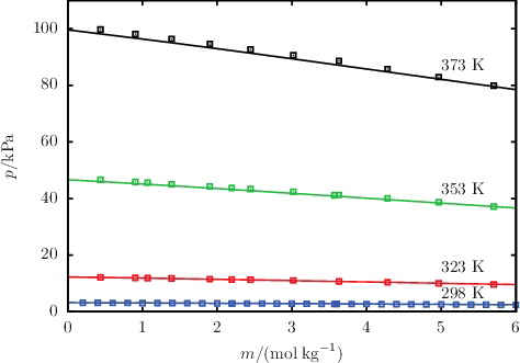
The description of osmotic coefficients of a range of 1:1 and 1:2 salts solutions, respectively, is illustrated in Figures 3 and 4, while the osmotic coefficients of acid and base solutions are shown in Figure 5. The SAFT-VR Mie calculations can be seen to follow the trends of the experimental data, with particularly good quantitative agreement in the highly non-ideal low-molality region. Liquid-phase densities at 298 and 323 K at 1.01 bar are shown in Figure 6 for a selection of aqueous salt solutions. The SAFT-VR Mie representation of the density allows us to assess the methodology for the choice of diameters used to describe the ions, since this property is heavily dependent on the sizes of the species in the mixture. We specifically assess the lithium salts because Li⁺ is the smallest ion considered in our work, and the assumptions made regarding the ion sizes are expected to have a greater impact for the smaller ions. Given the fair agreement between the calculated densities and experimental data, we conclude that the selected crystal ionic diameters can provide a reasonable estimate of the ion size. The calculated vapour pressures of aqueous NaCl for a range of temperatures are depicted in Figure 7, exemplifying the capability of the proposed model to reproduce the temperature dependence of the vapour pressure to a high level of accuracy. The results presented for these three key thermodynamic properties validate our implementation of the SAFT-VRE Mie approach for electrolytes, together with the ion models developed in our current work, as they are seen to provide a good description of the aqueous electrolyte solution properties across a broad range of conditions and compositions, with predictive capability well beyond the concentrations considered in the parameter estimation procedure.

Figure 3. The concentration dependence of the osmotic coefficient Φ for a selection of aqueous solutions of monovalent 1:1 salts at 298 K and 1.01 bar. The continuous curves represent the SAFT-VRE Mie calculations, and the squares represent the experimental data obtained from the sources listed in Table A3.

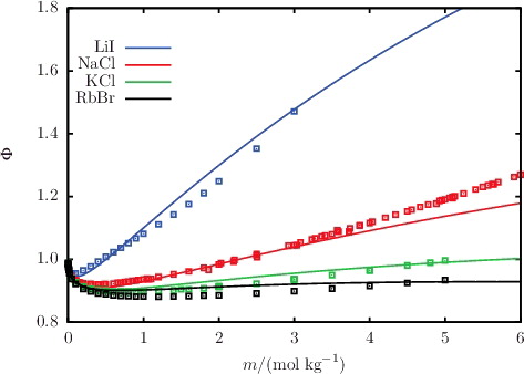
Figure 4. The concentration dependence of the osmotic coefficient Φ for a selection of aqueous solutions of 1:2 salts at 298 K and 1.01 bar. The continuous curves represent the SAFT-VRE Mie calculations, and the squares represent the experimental data obtained from the sources listed in Table A3.

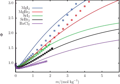
Figure 5. The concentration dependence of the osmotic coefficient Φ for aqueous solutions of acids and bases at 298 K and 1.01 bar. The continuous curves represent the SAFT-VRE Mie calculations, and the squares represent the experimental data obtained from the sources listed in Table A3.

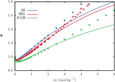
Figure 6. The concentration dependence of the liquid-phase density ρ for aqueous solutions of lithium salts LiI, LiBr, and LiCl. The continuous curves and squares represent the SAFT-VRE Mie calculations and experimental data, respectively, at 298 K and 1.01 bar. The dashed curves and circles represent the SAFT-VRE Mie calculations and experimental data at 323 K and 1.01 bar. The experimental data are obtained from the sources listed in Table A3.

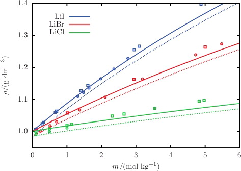
Figure 7. The concentration dependence of the saturated vapour pressure p for aqueous solutions of NaCl for temperatures ranging from 298 to 373 K. The continuous curves represent the SAFT-VR Mie calculations, and the squares represent the experimental data obtained from the sources listed in Table A3.

5.2. Mean ionic activity coefficient and osmotic coefficient

A direct way of assessing the reliability of the ion models and the predictive capability of the SAFT-VRE Mie approach is via the MIAC of the aqueous salts, which is directly related to the chemical potential of the solvated ions and consequently provides a measure of how well the thermodynamic properties of the ions are represented in solution. In our current work, the MIAC is not used in the development of the ion models, and the prediction of this property can hence serve as a benchmark for ensuring that the model parameters are physically sound.

The MIAC of aqueous solution of selected salts, acids, and bases are shown in Figures 8–10; the %AAD of the predicted values from the corresponding experimental data for all of the salts considered are reported in Table 7. The SAFT-VRE Mie predictions for the MIAC are in excellent agreement with the experimental data despite not having been considered in the model development. By limiting the molality range of the dataset used in the parameter estimation procedure, the non-ideality of the solution at low salinity is well accounted for. As a result, this leads to very good predictions for the MIAC. Four isotherms of the MIAC of aqueous NaCl solutions are shown in Figure 11 for temperatures in the range 288–333 K [82–88]. Correctly representing the experimental trend at low concentrations, SAFT-VRE Mie allows one to predict the decrease of the MIAC with increasing temperature for aqueous solutions of NaCl, thereby illustrating the predictive capability of the approach. At high salt concentrations, the SAFT-VRE Mie predictions continue to follow the temperature trend in the low-salinity region, which appears to be at odds with the experimental trend where the MIAC at 333 K is seen to become larger than that at 288 K; the deviations of the theoretical predictions from the experimental data are ∼20% at the highest concentrations considered. We should note, however, that there is a certain amount of scatter in the experimental data at high salinity, and that the trend for the MIAC is inconsistent with that observed for the osmotic coefficient Φ in Figure 12. As the MIAC and Φ are directly related through Equation (30(30) ), one would expect a similar trend with temperature, casting some doubt on the quality of the experimental data for the MIAC at higher temperatures and concentrations. On the other hand, the approximate description of the polarity of the solvent with a dielectric continuum in the SAFT-VRE approach is expected to be less adequate at very high salt concentrations.

Figure 8. The concentration dependence of the mean ionic activity coefficient γ_{±, m} for a selection of aqueous solutions of monovalent 1:1 salts at 298 K and 1.01 bar. The continuous curves represent the SAFT-VR Mie predictions, and the squares represent the experimental data obtained from the sources listed in Table A3.

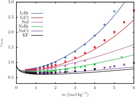
Figure 9. The concentration dependence of the mean ionic activity coefficient γ_{±, m} for a selection of aqueous solutions of 1:2 salts at 298 K and 1.01 bar. The continuous curves represent the SAFT-VR Mie predictions, and the squares represent the experimental data obtained from the sources listed in Table A3.

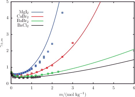
Figure 10. The concentration dependence of the mean ionic activity coefficient γ_{±, m} for a selection of aqueous solutions of acids and bases at 298 K and 1.01 bar. The continuous curves represent the SAFT-VR Mie predictions, and the squares represent the experimental data obtained from the sources listed in Table A3.

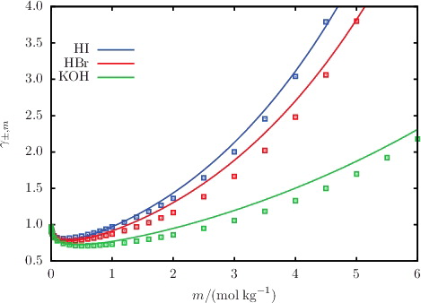
Figure 11. The concentration dependence of the mean ionic activity coefficient γ_{±, m} for aqueous solutions of NaCl at 1.01 bar for temperatures ranging from 288 to 333 K, shown both at low (top) and high (bottom) salinity. The continuous curves represent the SAFT-VR Mie predictions, and the squares represent the experimental data [82–88].

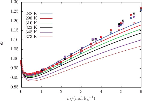
Figure 12. The concentration dependence of the osmotic coefficient Φ for aqueous solutions of NaCl at 1.01 bar for temperatures ranging from 288 to 373 K. The continuous curves represent the SAFT-VR Mie predictions, and the squares represent the experimental data obtained from the sources listed in Table A3.

5.3. Gibbs free energy of solvation

Our approach for the implementation of the Born contribution in the SAFT-VRE Mie EOS is evaluated by assessing the description of the Gibbs free energy of solvation ΔG_{solv, i} of the individual ions i in aqueous solution. The predictions of ΔG_{solv, i} are presented in Table 8, alongside the experimentally determined values obtained from [77–79]. These predictions are a significant improvement over those achieved in the previous implementation of SAFT-VRE [21], where the Born diameter was not differentiated from the segment diameter of the ion.

Table 8. Free energy of solvation ΔG_{solv, i} of ions i in aqueous solution: the SAFT-VRE Mie predictions are compared to the experimentally derived values reported in [77–79].

	−ΔGsolv, i/(kJ mol^− 1)
Ion, i	SAFT-VR Mie	Experiment
Li^+	535.72	529.00
Na^+	403.85	424.00
H3O^+	461.92	461.39
K^+	304.00	352.00
Rb^+	283.55	329.00
F^−	444.60	429.00
OH^−	432.58	437.94
Cl^−	313.04	304.00
Br^−	286.54	278.00
I^−	249.59	243.00
Ba^2 +	1331.45	1250.00
Ca^2 +	1524.81	1505.00
Mg^2 +	1946.03	1830.00
Sr^2 +	1378.75	1380.00

By adhering to the appropriate definition of the Born diameter as the cavity formed by the ion in the solvent, we show that it is possible to obtain not only qualitative agreement with the trend of the solvation energies, but also good quantitative agreement with the experimental values. The level of description of the solvation effects achieved with our current implementation of SAFT-VRE Mie is similar to that of SAFT approaches in which one treats the polarity of ion–solvent interactions explicitly [17,28,89].

5.4. Aqueous solubility of salts

In addition to the Gibbs free energy of solvation, it is also interesting to consider the limit of solubility of the salt, which can be calculated with a classical thermodynamic approach from knowledge of the activity coefficients of the ions using Equation (41(41) ). This requires the activity coefficients of the ions, which are calculated using the SAFT-VRE Mie methodology, as well as the solubility product K_{sp, MX} of the salt MX. One way of estimating K_{sp, MX} is via tabulated data for the Gibbs free energies of formation ΔG^f of the species using Equation (42(42) ). The ΔG^f of the salts and ions considered here are taken from the literature [90] and are summarised in Table 9. It is important to note that these values should be used with caution as they are not direct experimental measurements and are reported as ‘best’ estimates rather than absolute quantities. Alternatively, the experimental solubility product K_{sp, MX}^exp. can be calculated directly from experimental data for the mean ionic activity coefficient of the salt in saturated aqueous solution, by rearrangement of Equation (41(41) ): (55) The solubility product of a salt obtained from Equation (55(55) ) can be used with greater confidence since the data used in the calculation is specific to the salt in question. The experimental data for γ^exp_{±, m} at salt saturation are obtained from [91–100], and the values of K_sp calculated from Equation (55(55) ) or taken from [101] are presented in Table 10.

Table 9. Values used in Equation (41(41) ) for the Gibbs free energies of formation of the solid salts and solvated ions obtained from [90]. The of the salts correspond to the crystalline anhydrous salt at 298 K and 1.01 bar; and the of the ions correspond to the ion in aqueous solution at unit molality at 298 K and 1.01 bar.

Salt	− ΔG^fsalt(s)/(kJ mol^− 1)	Ion	− ΔG^fion(aq)/(kJ mol^− 1)
LiCl	384.37	Li^+	293.31
LiBr	342.00	Na^+	261.91
LiI	270.29	K^+	283.27
NaF	543.49	Rb^+	283.98
NaCl	384.14	F^−	278.79
NaBr	348.98	Cl^−	131.23
NaI	286.06	Br^−	103.96
KCl	409.14	I^−	51.57
KBr	380.66	Ca^2 +	533.58
KI	324.89	Sr^2 +	559.48
RbCl	407.80
RbBr	381.79
CaCl2	748.10
CaBr2	663.60
SrCl2	781.10

Table 10. Values for the experimental solubility product K_sp^exp. at 298 K and 1.01 bar used for the calculation of the solubilities of the salts in aqueous solution.

Salt	Ksp^exp.	Salt	Ksp^exp.
LiCl	1.388 × 10^6^a	CaCl2	1.309 × 10^7^a
LiBr	1.021 × 10^8^a	CaBr2	1.011 × 10^11^a
LiI	2.180 × 10^6^a	SrCl2	459.3^a
NaF	3.397 × 10^−1^a
NaCl	38.05^b
NaBr	114.7^b
KCl	8.003^b
KBr	13.53^b
KI	48.82^a
RbCl	20.24^a

^aValues calculated using Equation (55(55) ).

^bValues taken from [101].

We predict the solubility limits at 298 K and 1.01 bar for a number of aqueous salt solutions using the solubility equation with the solubility product obtained from both Equations (42(42) ) and (55(55) ); the results are presented in Table 11 alongside the experimental solubility data [70,102–104]. It is immediately evident that our predicted solubilities for the most commonly studied salts are in better agreement with the reported experimental solubilities than for the less commonly encountered salts; it is possible that the tabulated reference data for the Gibbs free energy of formation and the solubility product for the more common salts are more reliable. This is supported by the fact that for the common salts, the two routes for the calculation of the solubility lead to similar predicted values. We should also point out that many of salts considered here have a solubility limit which is well above the salt concentration for which SAFT-VRE Mie is applicable. The range of application for the SAFT-VRE Mie approach is estimated to be at a maximum salt molality of about 10 mol kg⁻¹ [21], assuming a solvation shell for the ions with six coordinated water molecules. Beyond this salt concentration, the dielectric constant of the mixture can no longer be expected to be the same as that of the pure solvent, as is inherently assumed in our approach. As a consequence, it is not surprising that we find better predictions of the solubility limit for the salts with a solubility which falls within the limits of applicability of the theory. By contrast, for salts which have a solubility limit well beyond the capability of SAFT-VRE Mie, such as lithium salts, the solubility is highly overpredicted.

Table 11. The solubility limit m^sat for aqueous solutions of salts at 298 K and 1.01 bar. The SAFT-VRE Mie predictions are compared to the experimentally obtained values reported in [70,102–104]. The dashes denote that the K_sp^exp. for the salt is unavailable.

	m^sat/(mol kg^−1)
	SAFT-VRE Mie
	Using ΔG^f	Using Ksp^exp.
Salt	(cf. Equation (42(42) ))	(cf. Equation (55(55) ))	Experiment
LiCl	49.11	34.16	19.94
LiBr	138.0	64.93	20.83
LiI	468.51	24.71	12.35
NaF	1.010	1.039	0.980
NaCl	6.830	6.900	6.150
NaBr	17.33	12.50	9.190
NaI	54.87	–	12.28
KCl	4.870	4.683	4.770
KBr	5.963	5.761	5.700
KI	10.73	10.07	8.920
RbCl	8.518	8.61	7.717
RbBr	7.072	–	6.916
RbI	6.855	–	7.630
CaCl2	10.65	8.571	7.320
CaBr2	44.47	13.29	7.820
SrCl2	11.56	3.825	3.350

6. Conclusions

The SAFT-VR Mie expression for the Helmholtz free energy of a mixture is combined with the mean-spherical approximation for a non-restricted primitive model of an electrolyte solution. The proposed molecular model includes the solvent explicitly; in this instance, the solvent is water, which is modelled in the usual SAFT manner, as spherical (and non-polar) with association sites to mediate hydrogen-bonding attractive interactions in addition to repulsive and dispersive attractive interactions described with a Mie (generalised Lennard-Jones) potential. The ion–ion interactions are included via Coulombic interactions as well as repulsive and dispersive interactions (of the Mie potential form). Ion–solvent (ion–water) interactions are also incorporated; the repulsive and dispersive interactions are again taken to be of the Mie form, and the contribution to the Helmholtz free energy accounting for the charging of the ion in the solvent is included via the classical expression presented by Born. We refer to our novel generalised description of electrolyte systems as the SAFT-VRE Mie approach.

By combining literature values of ionic sizes with a well-founded physical description of the molecular interactions, the parameterisation of ionic models for the electrolyte solutions is significantly simplified. Each model requires only one ion–solvent interaction parameter, in this case the unlike dispersion attractive energy, to be adjusted using experimental data for the ionic solution. We chose to limit the range of concentration considered for the determination of this parameter to less than three molal in order to adhere to the inherent assumptions of the MSA primitive model, i.e. the representation of the solvent as a uniform dielectric medium, and the assumption of complete dissociation of the ionic species. We note the importance of a careful evaluation of the experimental data used for the determination of the interaction parameters and the range of concentrations considered. The performance of the resulting approach is shown to be accurate, even when higher molalities are considered. The thermodynamic properties of the aqueous electrolyte solutions such as the density, vapour pressure, and osmotic coefficient are reproduced well. Furthermore, the robustness and thermodynamic consistency of the approach is demonstrated by the high level of accuracy seen in the predictions of the mean ionic activity coefficient for a range of salts, in comparison to available experimental data. It is also of interest to highlight the improved agreement in the prediction of the Gibbs free energy of solvation of the ions, which is obtained by incorporating information of the cavity size required for the insertion of the charged species in the solvent. The diameter of the cavity is taken from literature sources, or correlated from a linear relationship between the solvation energy and the size of the ion when data are not available.

We demonstrate the reliability of the SAFT-VRE Mie approach in modelling the thermodynamic properties of aqueous solutions of strong electrolytes, including salts of monovalent as well as divalent ions. The models presented for the ions are shown to be robust, in the sense that the predictive capability for properties not considered in the development of the models has been confirmed; the parameters are also fully transferable to different parent salts. Importantly, the ion potential models obtained are seen to be physically realistic. This is achieved by introducing experimental information for a number of the model parameters; experimentally derived quantities such as the ionic and Born diameters are used directly, while experimental ionisation potentials, polarisabilities, and electron affinities inform ion–ion energetic parameters through the use of a theoretical relation developed in previous work [66]. The number of adjustable parameters has therefore been reduced, compared with the previous formulation of SAFT-VRE SW [21]. As a guiding principle, this will prove of great value in future work considering ions for which experimental data are scarce, as well as offering greater confidence in the prediction of thermodynamic properties in regions where experimental measurements are unavailable.

Data statement

Data underlying this article can be accessed on Zenodo at https://zenodo.org/record/155809, and used under the Creative Commons Attribution license.

Acknowledgments

We would like to thank T. Laffite for very useful discussions related to this work. This work was carried out as part of the Qatar Carbonates and Carbon Storage Research Centre (QCCSRC). DKE and AJH are grateful for the funding of the QCCSRC provided jointly by Qatar Petroleum, Shell, and the Qatar Science & Technology Park, for the support of a PhD studentship and research fellowship, respectively. GL is thankful to Pfizer Inc. for funding a PhD studentship. Additional support to the Molecular Systems Engineering Group from the Engineering and Physical Science Research Council (EPSRC) of the United Kingdom is also gratefully acknowledged.

Disclosure statement

No potential conflict of interest was reported by the authors.

Additional information

Funding

The funding of this study was provided by QCCSRC; Pfizer Inc.; Qatar Petroleum; Shell; the Qatar Science and Technology Park; the Engineering and Physical Science Research Council (EPSRC) of the United Kingdom [grant number GR/T17595], [grant number GR/N35991], [grant number EP/E016340], [grant number EP/J014958]; the Joint Research Equipment Initiative (JREI) [GR/M94426]; and the Royal Society-Wolfson Foundation.

Appendix

Table A1. Overview of the experimental aqueous electrolyte solution data considered in the estimation procedure for the development of the SAFT-VRE Mie ion models. The ranges of temperatures T, maximum molality m_max, and the number of data points n_p per property (saturated vapour pressure p, density ρ, and osmotic coefficient Φ) are summarised for each salt.

Salt MX		p				ρ			Φ
	T/K	mmax/ (mol kg^−1)	np	T/K	p/bar	mmax/ (mol kg^−1)	np	T/K	mmax/ (mol kg^−1)	np
KBr	298–368	2.8	30	283–348	1.01	3.0	188	298	3.0	23
KCl	298–368	3.0	74	278–353	1.01	3.0	48	298	3.0	36
KF	291	2.8	4	298	1.01	3.0	138	298	3.0	23
KI	303–343	3.0	24	278–368	1.01	1.0	283	298	3.0	23
LiBr	313–368	2.9	12	278–343	1.01	2.9	114	298	3.0	23
LiCl	293–423	3.0	31	278–343	1.01	2.7	200	298	3.0	43
LiI	291–343	2.5	13	298–373	1.01	3.0	74	298	3.0	23
NaBr	303–368	3.0	20	283–343	1.01	2.9	76	298	2.9	28
NaCl	283–383	3.0	100	283–353	1.01	3.0	48	298	3.0	52
NaF	373–448	0.01	24	298–323	1.01	0.9	161	298	1.0	17
NaI	298–368	2.7	28	293–303	1.01	1.7	34	298	3.0	23
RbBr	291	2.4	16	298–323	1.01	3.0	23	298	3.0	23
RbCl	263–368	3.0	32	298	1.01	3.0	23	298	3.0	23
RbF	291	2.6	5	298	1.01	0.5	7	298	3.0	23
RbI	291	2.7	9	298–310	1.01	0.4	15	298	3.0	23
HBr	298–327	2.6	6	298–348	1.01	3.0	78	298	3.0	42
KOH	293–473	3.0	8	298–348	1.01	3.0	73	298	3.0	23
MgBr2	373	3.0	4	298	–	2.9	12	298–323	3.0	46
MgCl2	295–394	3.0	140	288–372	–	2.9	118	298–343	3.0	65
MgI2	–	–	–	–	–	–	–	298	3.0	36
CaBr2	298–373	3.0	33	298	–	2.7	26	298–473	3.0	84
CaCl2	291–391	3.0	356	288–28	–	3.0	42	288–473	3.0	282
CaI2	298–343	2.9	29	–	–	–	–	–	–	–
SrBr2	303–373	3.0	39	298	–	2.4	13	298	2.1	40
SrCl2	303–343	2.9	30	–	–	–	-	298	3.0	36
SrI2	303–343	2.9	30	–	–	–	–	298	2.0	38
BaBr2	303–373	3.0	39	298	–	1.6	12	298–343	2.5	92
BaCl2	298–343	1.7	51	288–28	–	1.5	49	298–372	2.5	45
BaI2	–	–	–	–	–	–	–	298	2.0	38

Table A2. Overview of the experimental aqueous electrolyte solution data considered in the assessment of the SAFT-VRE Mie ion models. The ranges of temperatures T, maximum molality m_max, and the number of data points n_p per property (saturated vapour pressure p, density ρ, osmotic coefficient Φ, and mean ion activity coefficient γ_{±, m}) are summarized for each salt.

Salt		p				ρ			Φ			γ±, m
	T/K	mmax/(mol kg^−1)	np	T/K	p/bar	mmax/(mol kg^−1)	np	T/K	mmax/(mol kg^−1)	np	T/K	mmax/(mol kg^−1)	np
KBr	283–368	6.2	79	283–348	1.01	5.8	265	298–498	7.4	28	298	5.5	36
KCl	298–373	6.9	125	298–353	1.01	4.0	64	273–473	6.0	49	298	4.0	80
KF	291	9.2	9	297–372	1.01	8.9	167	298	10.0	23	298	4.0	15
KI	303–343	5.6	40	278–373	1.01	1.0	283	298–343	5.6	26	298	4.0	35
LiBr	291–373	9.8	94	278–343	1.01	10.0	249	298–498	10.0	33	298	9.0	34
LiCl	298–423	9.1	106	278–343	1.01	10.0	236	298–473	10.0	75	298	10.0	48
LiI	291–343	9.8	35	298–373	1–1.01	4.9	84	298	3.0	23	298	3.0	33
NaBr	283–368	9.9	71	283–343	1.01	8.3	162	298–473	9.5	100	298	8.2	47
NaCl	273–383	6.8	203	298–473	1.01	5.0	64	298–373	6.1	94	298	6.1	30
NaF	373–448	0.0	24	297–498	1.01	1.0	161	298	1.0	17	298	1.0	6
NaI	298–368	9.3	88	298	1.01	1.7	34	298	10.0	33	298	3.5	14
RbBr	263–368	4.8	32	298–323	1.01	6.8	27	298	5.0	27	298	5.0	32
RbCl	291	7.1	89	298	1.01	5.0	27	298	7.8	32	298	5.0	17
RbF	291	9.8	7	298	1.01	0.5	7	298	3.5	24	298	3.5	14
RbI	291	5.6	10	298–310	1.01	0.4	15	298	5.0	27	298	5.0	34
HCl	298–373	10.0	154	298–348	1.01	9.9	117	298	10.0	64	298	10.0	34
HBr	298–338	7.9	26	298–348	1.01	3.0	78	298	10.0	60	298	10.0	34
HI	298	8.8	5	298–348	1.01	2.5	79	298	10.0	33	298	10.0	34
NaOH	293–298	10.0	20	298–348	1.01	3.0	86	298	10.0	33	298	10.0	34
KOH	293–473	10.0	30	298–348	1.01	3.0	73	298	10.0	33	298	10.0	34
MgBr2	373	4.0	5	298	–	3.7	13	298–323	5.0	54	298	3.0	15
MgCl2	295–398	5.0	210	288–372	–	4.8	153	298–343	5.0	95	298	5.9	53
MgI2	–	–	–	–	–	–	–	298	5.0	44	298	1.6	13
CaBr2	298–373	5.7	53	298	–	3.4	27	298–473	5.0	100	298	3.0	15
CaCl2	291–403	5.0	541	288–328	-	4.0	49	288–498	5.4	362	298	3.0	67
CaI2	298–343	2.9	29	–	–	–	–	–	–	–	298	1.8	14
SrBr2	303–373	4.0	45	298	–	2.4	13	298	2.1	40	298	2.0	30
SrCl2	303–343	4.2	40	–	–	–	–	298	4.0	42	298	4.0	78
SrI2	303–343	4.2	40	–	–	–	–	298	2.0	38	298	2.0	30
BaBr2	303–373	3.4	44	298	–	1.6	12	298–343	3.4	97	278–318	2.3	49
BaCl2	298–343	1.7	51	288–328	–	1.5	49	298–372	2.5	45	298	1.4	14
BaI2	–	–	–	–	–	–	–	298	2.0	38	298	2.0	30

Table A3. Sources of the experimental aqueous electrolyte solution data summarised in Tables A1 and A2.

Salt	p	ρ	Φ	γ±, m
KBr	[105–108]	[109–112]	[97]	[97]
KCl	[96,104,106–108,113,114]	[110,112]	[97,115–117]	[97]
KF	[118]	[119–121]	[97]	[97]
KI	[106]	[119,120,122–124]	[97,106]	[97]
LiBr	[107,125–128]	[110,111,129]	[97,130]	[97]
LiCl	[107,131–133]	[110,134,135]	[97,136]	[97]
LiI	[118,126]	[137–139]	[97]	[97]
NaBr	[105–107]	[110,111,140]	[97,130,141]	[97]
NaCl	[96,142,143]	[110,112]	[97,115,141,143–146]	[97]
NaF	[147]	[119–121,148]	[97]	[97]
NaI	[106,107,149]	[119,120,150,151]	[97]	[97]
RbBr	[118,152]	[119,153,154]	[97]	[97]
RbCl	[106,107,118,152]	[120,150,155]	[97]	[97]
RbF	[118]	[119]	[97]	[97]
RbI	[118]	[119,156]	[97]	[97]
HCl	[157–159]	[160,161]	[97,158]	[158]
HBr	[162,163]	[160]	[97,164]	[97]
HI	[165]	[160]	[97]	[97]
NaOH	[133]	[166,167]	[97]	[97]
KOH	[133,168]	[166,169]	[97]	[97]
MgBr2	[170]	[171]	[172]	[173]
MgCl2	[106,170,174–176]	[177,178]	[106,179]	[179,180]
MgI2	–	–	[172]	[99,181]
CaBr2	[106,165,170]	[171,182]	[183]	[173,183]
CaCl2	[106,170,175,176,184–193]	[194]	[98,106,145,183,195–198]	[95,173,183,199,200]
CaI2	[106,165]	–	–	[99]
SrBr2	[106,170]	[171]	[172]	[99,201]
SrCl2	[106]	–	[172]	[202–204]
SrI2	[106]	–	[172]	[99,201]
BaBr2	[106,170]	[171]	[99,106,172]	[173,205]
BaCl2	[106,185]	[194]	[172,206]	[173]
BaI2	–	–	[172]	[99,201]

References

- E. Debye and P. Hückel, Phys. Z. 24, 179 (1923).
- M. Gouy, J. Phys. 9, 457 (1910).
- D.L. Chapman, Phil. Mag. 25, 475 (1913).
- E. Waisman and J.L. Lebowitz, J. Chem. Phys. 52, 4307 (1970).
- L. Blum, J. Chem. Phys. 61, 2129 (1974).
- L. Blum, Mol. Phys. 30, 1529 (1975).
- L. Blum and D.Q. Wei, J. Chem. Phys. 87, 555 (1987).
- W.G. Chapman, K.E. Gubbins, G. Jackson, and M. Radosz, Ind. Eng. Chem. Res. 29, 1709 (1990).
- W.G. Chapman, K.E. Gubbins, G. Jackson, and M. Radosz, Fluid Phase Equilib. 52, 31 (1989).
- G.M. Kontogeorgis, E.C. Voutsas, I.V. Yakoumis, and D.P. Tassios, Ind. Eng. Chem. Res. 35, 4310 (1996).
- J. Wu and J.M. Prausnitz, Ind. Eng. Chem. Res. 37, 1634 (1998).
- W.B. Liu, Y.G. Li, and J.F. Lu, Fluid Phase Equilib. 158–160, 595 (1999).
- A. Galindo, A. Gil-Villegas, G. Jackson, and A.N. Burgess, J. Phys. Chem. B 103, 10272 (1999).
- B.H. Patel, P. Paricaud, A. Galindo, and G.C. Maitland, Ind. Eng. Chem. Res. 42, 3809 (2003).
- B. Behzadi, B. Patel, A. Galindo, and C. Ghotbi, Fluid Phase Equilib. 236, 241 (2005).
- L.F. Cameretti, G. Sadowski, and J.M. Mollerup, Ind. Eng. Chem. Res. 44, 3355 (2005).
- H. Zhao, M.C. dos Ramos, and C. McCabe, J. Chem. Phys. 126, 244503 (2007).
- C. Held, L.F. Cameretti, and G. Sadowski, Fluid Phase Equilib. 270, 87 (2008).
- C. Held and G. Sadowski, Fluid Phase Equilib. 279, 141 (2009).
- J. Rozmus, J.C. de Hemptinne, A. Galindo, S. Dufal, and P. Mougin, Ind. Eng. Chem. Res. 52, 9979 (2013).
- J.M.A. Schreckenberg, S. Dufal, A.J. Haslam, C.S. Adjiman, G. Jackson, and A. Galindo, Mol. Phys. 112, 2339 (2014).
- B. Maribo-Mogensen, K. Thomsen, and G.M. Kontogeorgis, AIChE J. 61, 2933 (2015).
- S.A. Adelman and J. Deutch, J. Chem. Phys. 59, 3971 (1973).
- S.A. Adelman and J.M. Deutch, J. Chem. Phys. 60, 3935 (1974).
- M. Born, Z. Phys. 1, 45 (1920).
- Y. Lin, K. Thomsen, and J.C. de Hemptinne, AIChE J. 53, 989 (2007).
- R. Inchekel, J.C. de Hemptinne, and W. Fürst, Fluid Phase Equilib. 271, 19 (2008).
- S. Herzog, J. Gross, and W. Arlt, Fluid Phase Equilib. 297, 23 (2010).
- G. Das, S. Hlushak, M.C. dos Ramos, and C. McCabe, AIChE J. 61, 3053 (2015).
- G. Das, S. Hlushak, and C. McCabe, Fluid Phase Equilib. 416, 72 (2016).
- B. Maribo-Mogensen, G.M. Kontogeorgis, and K. Thomsen, J. Phys. Chem. B 117, 10523 (2013).
- B. Maribo-Mogensen, G.M. Kontogeorgis, and K. Thomsen, J. Phys. Chem. B 117, 3389 (2013).
- A. Gil-Villegas, A. Galindo, P.J. Whitehead, S.J. Mills, G. Jackson, and A.N. Burgess, J. Chem. Phys. 106, 4168 (1997).
- A. Galindo, L. Davies, A. Gil-Villegas, and G. Jackson, Mol. Phys. 93, 241 (1998).
- G. Mie, Ann. Phys. (Berlin, Ger.) 316, 657 (1903).
- T. Lafitte, A. Apostolakou, C. Avendaño, A. Galindo, C.S. Adjiman, E.A. Müller, and G. Jackson, J. Chem. Phys. 139, 154504 (2013).
- S. Dufal, T. Lafitte, A.J. Haslam, A. Galindo, G.N.I. Clark, C. Vega, and G. Jackson, Mol. Phys. 113, 948 (2015).
- S. Dufal, T. Lafitte, A. Galindo, G. Jackson, and A.J. Haslam, AIChE J. 61, 2891 (2015).
- V. Papaioannou, T. Lafitte, C. Avendaño, C.S. Adjiman, G. Jackson, E.A. Müller, and A. Galindo, J. Chem. Phys. 140, 054107 (2014).
- S. Dufal, V. Papaioannou, M. Sadeqzadeh, T. Pogiatzis, A. Chremos, C. Adjiman, G. Jackson, and A. Galindo, J. Chem. Eng. Data 59, 3272 (2014).
- M.S. Wertheim, J. Stat. Phys. 35, 19 (1984).
- M.S. Wertheim, J. Stat. Phys. 35, 35 (1984).
- M.S. Wertheim, J. Stat. Phys. 42, 459 (1986).
- M.S. Wertheim, J. Stat. Phys. 42, 477 (1986).
- G. Jackson, W.G. Chapman, and K.E. Gubbins, Mol. Phys. 65, 1 (1988).
- W.G. Chapman, G. Jackson, and K.E. Gubbins, Mol. Phys. 65, 1057 (1988).
- L.L. Lee, Molecular Thermodynamics of Nonideal Fluids (Butterworth, Boston, MA, 1988).
- J.A. Barker and D. Henderson, J. Chem. Phys. 47, 2856 (1967).
- T. Boublík, J. Chem. Phys. 53, 471 (1970).
- G.A. Mansoori, J. Chem. Phys. 54, 1523 (1971).
- B.J. Zhang, Fluid Phase Equilib. 154, 1 (1999).
- P. Paricaud, J. Chem. Phys. 124, 154505 (2006).
- M.S. Wertheim, J. Chem. Phys. 87, 7323 (1987).
- E. Waisman, J. Chem. Phys. 56, 3086 (1972).
- L. Blum and J.S. Hoye, J. Phys. Chem. 81, 1311 (1977).
- B. Maribo-Mogensen, G.M. Kontogeorgis, and K. Thomsen, Ind. Eng. Chem. Res. 51, 5353 (2012).
- A.H. Harvey and J.M. Prausnitz, J. Solution Chem. 16, 857 (1987).
- G.M. Kontogeorgis and G.K. Folas, Thermodynamic Models for Industrial Applications: From Classical and Advanced Mixing Rules to Association Theories, 2nd ed. (Wiley, New York, 2010).
- J.M. Prausnitz, R.N. Lichtenthaler, and E.G. de Azevedo, Molecular Thermodynamics of Fluid-Phase Equilibria (Prentice-Hall, Inc., Englewood Cliffs, NJ, 1998).
- C. Großmann and G. Maurer, Fluid Phase Equilib. 106, 17 (1995).
- D.W. Marquardt, J. Soc. Ind. Appl. Math. 11, 431 (1963).
- K. Levenberg, Q. Appl. Math. 2, 164 (1944).
- A. Gil-Villegas, A. Galindo, and G. Jackson, Mol. Phys. 99, 531 (2001).
- A.A. Rashin and B. Honig, J. Phys. Chem. 89, 5588 (1985).
- G.H. Hudson and J. McCoubrey, Trans. Faraday Soc. 56, 761 (1960).
- A.J. Haslam, A. Galindo, and G. Jackson, Fluid Phase Equilib. 266, 105 (2008).
- F. London, Trans. Faraday Soc. 33, 8b (1937).
- J.E. Lennard-Jones, Proc. Phys. Soc. 43, 461 (1931).
- R. Heyrovská, Mar. Chem. 70, 49 (2000).
- D.R. Lide, editor, CRC Handbook of Chemistry and Physics, 86th ed. (CRC Press, London, UK, 2005).
- S. Klein, E. Kochanski, and A. Strich, Chem. Phys. Lett. 260, 34 (1996).
- M.I. Al-Joboury and D.W. Turner, J. Chem. Soc. B: Physical Organic, 1, 373–376 (1967).
- N. Pyper, C. Pike, and P. Edwards, Mol. Phys. 76, 353 (1992).
- L.M. Branscomb, Phys. Rev. 148, 11 (1966).
- R.D. Shannon, Acta Crystallogr. A 32, 751 (1976).
- H.C. Helgeson and D.H. Kirkham, Am. J. Sci. 276, 97 (1976).
- Y. Marcus, J. Chem. Soc., Faraday Trans. 87, 2995 (1991).
- W.R. Fawcett, J. Phys. Chem. B 103, 11181 (1999).
- D.M. Camaioni and C.A. Schwerdtfeger, J. Phys. Chem. A 109, 10795 (2005).
- O. Markovith and N. Agmon, J. Phys. Chem. A 111, 2253 (2007).
- W.H. Robertson, E.G. Diken, E.A. Price, J.W. Shin, and M.A. Johnson, Science 299, 1367 (2003).
- H.S. Harned and L.F. Nims, J. Am. Chem. Soc. 54, 423 (1932).
- H.S. Harned and M.A. Cook, J. Am. Chem. Soc. 61, 495 (1939).
- G. Janz and A. Gordon, J. Am. Chem. Soc. 65, 218 (1943).
- U. Westhaus, T. Dröge and R. Sass, Fluid Phase Equilib. 158, 429 (1999).
- X. Ji, X. Lu, S. Li, L. Zhang, Y. Wang, and J. Shi, J. Solution Chem. 30, 463 (2001).
- F. Sirbu, O. Iulian, A.C. Ion, and I. Ion, J. Chem. Eng. Data 56, 4935 (2011).
- J. Yao, W.D. Yan, Y.J. Xu, and S.J. Han, J. Chem. Eng. Data 44, 497 (1999).
- Z. Liu, W. Wang, and Y. Li, Fluid Phase Equilib. 227, 147 (2005).
- D.D. Wagman, W.H. Evans, V.B. Parker, R.H. Schumm, and I. Halow, J. Phys. Chem. Ref. Data 11, Supplement 2 (1982).
- V. Filippov, L. Vivcharik, and E. Gubanikhin, Russ. J. Inorg. Chem. 20, 941 (1975).
- Y. Yao, B. Sun, P.S. Song, Z. Zhang, R.L. Wang, and J.Q. Chen, Acta Chim. Sinica 50, 839 (1992).
- J.N. Pearce and A.F. Nelson, J. Am. Chem. Soc. 54, 3544 (1932).
- F. Hernández-Luis, R. Rodríguez-Raposo, and D. Grandoso, J. Chem. Eng. Data 56, 3940 (2011).
- K. Zhuo, H. Liu, H. Zhang, Y. Liu, and J. Wang, J. Chem. Thermodyn. 40, 889 (2008).
- J.I. Partanen and A.K. Covington, J. Chem. Eng. Data 54, 208 (2008).
- W.J. Hamer and Y.C. Wu, J. Phys. Chem. Ref. Data 1, 1047 (1972).
- J.A. Rard and S.L. Clegg, J. Chem. Eng. Data 42, 819 (1997).
- R. Stokes, Trans. Faraday Soc. 44, 259 (1948).
- J.A. Rard, J. Chem. Eng. Data 29, 443 (1984).
- X. Ji, S.P. Tan, H. Adidharma, and M. Radosz, Ind. Eng. Chem. Res. 44, 7584 (2005).
- C. Balarew, C. Christov, V. Valyashko, and S. Petrenko, J. Solution Chem. 22, 173 (1993).
- Y. Vlasov and B. Seleznev, Russ. J. Phys. Chem. 45, 772 (1971).
- A. Apelblat, J. Chem. Thermodyn. 30, 1191 (1998).
- A. Apelblat, J. Chem. Thermodyn. 25, 63 (1993).
- K.R. Patil, A.D. Tripathi, G. Pathak, and S.S. Katti, J. Chem. Eng. Data 36, 225 (1991).
- K.R. Patil, F. Olivé, and A. Coronas, J. Chem. Eng. Jpn. 27, 680 (1994).
- V. Filippov, M. Yakimov, V. Makarevskii, and L. Lukina, Russ. J. Inorg. Chem. 16, 1653 (1971).
- I.M. Abdulagatov and N.D. Azizov, Fluid Phase Equilib. 246, 96 (2006).
- J. Kiepe, A. Karine de Araújo Rodrigues, S. Horstmann, and J. Gmehling, Ind. Eng. Chem. Res. 42, 2022 (2003).
- N. Rohman, N.N. Dass, and S. Mahiuddin, J. Mol. Liq. 100, 265 (2002).
- M. Taha and M.J. Lee, J. Chem. Thermodyn. 41, 705 (2009).
- S. Behme, G. Sadowski and W. Arlt, Chem. Ing. Tech. 67, 757 (1995).
- T.M. Herrington and R.J. Jackson, J. Chem. Soc. Faraday Trans. 1 69, 1635 (1973).
- E. Amado and L.H. Blanco, Fluid Phase Equilib. 226, 261 (2004).
- S. Manohar, J. Ananthaswamy, and G. Atkinson, J. Chem. Soc. Faraday Trans. 88, 991 (1992).
- R.T. Pabalan and K.S. Pitzer, J. Chem. Eng. Data 33, 354 (1988).
- A. Lannung, Z. Phys. Chem. Abt. A 170, 134 (1934).
- J.E. Desnoyers, M. Arel, G. Perron, and C. Jolicoeur, J. Phys. Chem. 73, 3346 (1969).
- F.J. Millero, G.K. Ward, and P.V. Chetirkin, J. Acoust. Soc. Am. 61, 1492 (1977).
- T.G. Pedersen, C. Dethlefsen, and A. Hvidt, Carlsberg Res. Commun. 49, 445 (1984).
- A. Apelblat and E. Manzurola, J. Mol. Liq. 118, 77 (2005).
- L. Dunn, Trans. Faraday Soc. 64, 1898 (1968).
- D. Out and J. Los, J. Solution Chem. 9, 19 (1980).
- D.A. Boryta, A.J. Maas, and C.B. Grant, J. Chem. Eng. Data 20, 316 (1975).
- K.R. Patil, A.D. Tripathi, G. Pathak, and S.S. Katti, J. Chem. Eng. Data 35, 166 (1990).
- M. Renz, Ph.D. thesis, DKV Report No. 5, Stuttgart, 1980.
- E. Sada, T. Morisue, and K. Miyahara, J. Chem. Eng. Jpn. 8, 196 (1975).
- M.M. Palaiologou, I.E. Molinou, and N.G. Tsierkezos, J. Chem. Eng. Data 47, 1285 (2002).
- H. Holmes and R. Mesmer, J. Chem. Thermodyn. 30, 723 (1998).
- A.N. Campbell and O.N. Bhatnagar, Can. J. Chem. 57, 2542 (1979).
- S.K. Chaudhari and K.R. Patil, Phys. Chem. Liq. 40, 317 (2002).
- W. Kangro and A. Groeneveld, Z. Phys. Chem. 32, 110 (1962).
- A. Apelblat and E. Manzurola, J. Chem. Thermodyn. 33, 1133 (2001).
- E. Vercher, S. Solsona, M.I. Vázquez, and A. Martınez-Andreu, Fluid Phase Equilib. 209, 95 (2003).
- H.F. Gibbard, Jr, and G. Scatchard, J. Chem. Eng. Data 18, 293 (1973).
- I.M. Abdulagatov and N.D. Azizov, J. Chem. Thermodyn. 36, 829 (2004).
- J. Safarov, J. Mol. Liq. 123, 139 (2006).
- D. Salavera, X. Esteve, K. Patil, A.M. Mainar, and A. Coronas, J. Chem. Eng. Data 49, 613 (2004).
- Y. Sanmamed, D. González-Salgado, J. Troncoso, C. Cerdeirina, and L. Romani, Fluid Phase Equilib. 252, 96 (2007).
- J.A. Rard and D.G. Archer, J. Chem. Eng. Data 40, 170 (1995).
- A. Mersrnann, Chem. Ing. Tech. 64, 585 (1992).
- K. Nasirzadeh, D. Zimin, R. Neueder, and W. Kunz, J. Chem. Eng. Data 49, 607 (2004).
- L.H. Blanco and A.P. Rozo, J. Solution Chem. 39, 1819 (2010).
- C.W. Childs and R.F. Platford, Aust. J. Chem. 24, 2487 (1971).
- H.F. Gibbard, Jr, G. Scatchard, R.A. Rousseau, and J.L. Creek, J. Chem. Eng. Data 19, 281 (1974).
- A.G. Guseinov, M.V. Imanova, R.T. Akhundov, A.D. Tairov, and A.I. Iskenderov, Izv. Vyssh. Uchebn. Zaved. Neft Gaz 9–10, 45 (1991).
- F.J. Millero and J.H. Knox, J. Chem. Eng. Data 18, 407 (1973).
- H. Yamamoto, T. Terano, M. Yanagisawa, and J. Tokunaga, Can. J. Chem. Eng. 73, 779 (1995).
- M. Palma and J.P. Morel, J. Solution Chem. 8, 767 (1979).
- K.L. Zho, Y. Zhao, L.X. Yang, Q. Liu, and J.J. Wang, J. Chin. Chem. Soc. 53, 961 (2006).
- A. Stagis and K.P. Mishchenko, J. Gen. Chem. USSR 40, 2127 (1970).
- G.P. Baxter and C.C. Wallace, J. Am. Chem. Soc. 38, 70 (1916).
- M.K. Karapetyants, V. Vasilev, B. Mikhailin, and V. Strakhov, Zh. Fiz. Khim. 53, 207 (1979).
- A. Ostroff, B. Snowden, Jr, and D. Woessner, J. Phys. Chem. 73, 2784 (1969).
- M. Singh and M. Pandey, J. Indian Chem. Soc. 82, 1091 (2005).
- F.C. Quiroz, Ph.D. thesis, RWTH Aachen, 1986.
- R. Haase, H. Naas, and H. Thumm, Z. Phys. Chem. 37, 210 (1963).
- M. Susarev and R. Prokofeva, Zh. Fiz. Khim. 37, 2408 (1963).
- T.M. Herrington, A.D. Pethybridge, and M.G. Roffey, J. Chem. Eng. Data 30, 264 (1985).
- P. Rizzo, J.G. Albright, and D.G. Miller, J. Chem. Eng. Data 42, 623 (1997).
- G. Wüster, G. Wozny, and Z. Giazitzoglou, Fluid Phase Equilib. 6, 93 (1981).
- N. Elm, J. Zipprian, and K. Schaber, Fluid Phase Equilib. 189, 163 (2001).
- J. Macaskill and R.G. Bates, J. Solution Chem. 12, 607 (1983).
- L.S. Lilich and M.D. Anikeeva, Zh. Neorg. Khim. 4, 2630 (1959).
- T.M. Herrington, A.D. Pethybridge, and M.G. Roffey, J. Chem. Eng. Data 31, 31 (1986).
- G. Vázquez, E. Alvarez, R. Varela, A. Cancela, and J.M. Navaza, J. Chem. Eng. Data 41, 244 (1996).
- V. Mashovets, B. Krumgalz, I. Dibrov, and R. Matveeva, Russ. J. Appl. Chem. 38, 2294 (1965).
- H. Corti, R.F. Prini, and F. Svarc, J. Solution Chem. 19, 793 (1990).
- G. Tammann, Z. Phys. Chem. (Leipzig) 2, 42 (1888).
- H.C. Jones and H.P. Bassett, Am. Chem. J. 33, 534 (1905).
- R.N. Goldberg and R.L. Nuttall, J. Phys. Chem. Ref. Data 7, 263 (1978).
- E. Rodil and J. Vera, Fluid Phase Equilib. 205, 115 (2003).
- Z. Adamcova and J. Farkova, Sb. Vys. Sk. Chem. Technol. Praze N Fyz. Chem. 7, 69 (1986).
- L. Lee, I. Ho, C. Lin, and C. Lin, J. Chin. Inst. Chem. Eng. 36, 271 (2005).
- T. Sako, T. Hakuta, and H. Yoshitome, J. Chem. Eng. Data 30, 224 (1985).
- A.L. Surdo, E.M. Alzola, and F.J. Millero, J. Chem. Thermodyn. 14, 649 (1982).
- P.P. Saluja, D.J. Jobe, J.C. LeBlanc, and R.J. Lemire, J. Chem. Eng. Data 40, 398 (1995).
- J.A. Rard and D.G. Miller, J. Chem. Eng. Data 26, 38 (1981).
- M.A. Bagherinia, M. Giahi, M. Pournaghdy, and G.R. Vaghar, J. Chem. Thermodyn. 44, 169 (2012).
- R. Robinson and R. Stokes, Trans. Faraday Soc. 6, 733 (1940).
- W. Grzybkowski and G. Atkinson, J. Chem. Eng. Data 31, 309 (1986).
- M.S. Gruszkiewicz and J.M. Simonson, J. Chem. Thermodyn. 37, 906 (2005).
- M.F. Bechtold and R.F. Newton, J. Am. Chem. Soc. 62, 1390 (1940).
- M. Filiz and J. Gülen, Fluid Phase Equilib. 267, 18 (2008).
- A. Lannung, Z. Anorg. Allg. Chem. 228, 1 (1936).
- B. Li, Y. Luo, and Z. Zhu, J. Chin. Inst. Chem. Eng. 1, 102 (1986).
- L.S. Lilich and M.D. Anikeeva, Vestn. Leningr. Univ. Ser. 4 Fiz. Khim. 4, 85 (1967).
- L.S. Lilich and M.D. Anikeeva, Vestn. Leningr. Univ. Ser. 4 Fiz. Khim. 22, 97 (1956).
- A. Mun, J. Gen. Chem. USSR 26, 1161 (1956).
- E. Plake, Z. Physik. Chem. A 172, 113 (1935).
- N.V. Sidgwick and E.K. Ewbank, J. Chem. Soc. Trans. 125, 2268 (1924).
- R. Stokes and R. Robinson, Ind. Eng. Chem. 41, 2013 (1949).
- T. Isono, J. Chem. Eng. Data 29, 45 (1984).
- R.F. Platford, J. Chem. Eng. Data 18, 215 (1973).
- H. McLeod and A. Gordon, J. Am. Chem. Soc. 68, 58 (1946).
- T.M. Davis, L.M. Duckett, C.E. Garvey, J.M. Hollifield, and C.S. Patterson, J. Chem. Eng. Data 31, 54 (1986).
- S. J. Baabor, M. Gilchrist, and Delgado, J. Chem. Thermodyn. 33, 405 (2001).
- J. Ma, X. Zhang, K. Zhuo, H. Liu, and J. Wang, J. Chem. Thermodyn. 42, 689 (2010).
- A. Schneider, C. Pasel, M. Luckas, K. Schmidt and J. Herbell, Chem. Ing. Tech. 75, 244 (2003).
- R. Robinson, Trans. Faraday Soc. 38, 445 (1942).
- J.A. Rard and D.G. Miller, J. Chem. Eng. Data 27, 169 (1982).
- J. Macaskill, D. White, Jr, R. Robinson, and R.G. Bates, J. Solution Chem. 7, 339 (1978).
- S.L. Clegg, J.A. Rard, and D.G. Miller, J. Chem. Eng. Data 50, 1162 (2005).
- R.N. Roy, L.N. Roy, W.B. Davis, D.W. Larkin, D. Willard, D.A. Johnson, and F.J. Millero, J. Chem. Thermodyn. 25, 155 (1993).
- C.S. Patterson, L. Gilpatrick, and B. Soldano, J. Chem. Soc. 2730–2734 (1960).