Computation of partial molar properties using continuous fractional component Monte Carlo

ABSTRACT

An alternative method for calculating partial molar excess enthalpies and partial molar volumes of components in Monte Carlo (MC) simulations is developed. This method combines the original idea of Frenkel, Ciccotti, and co-workers with the recent continuous fractional component Monte Carlo (CFCMC) technique. The method is tested for a system of Lennard–Jones particles at different densities. As an example of a realistic system, partial molar properties of a [NH₃, N₂, H₂] mixture at chemical equilibrium are computed at different pressures ranging from P = 10 to 80 MPa. Results obtained from MC simulations are compared to those obtained from the PC-SAFT Equation of State (EoS) and the Peng–Robinson EoS. Excellent agreement is found between the results obtained from MC simulations and PC-SAFT EoS, and significant differences were found for PR EoS modelling. We find that the reaction is much more exothermic at higher pressures.

GRAPHICAL ABSTRACT

KEYWORDS:

• Molecular simulation
• partial molar properties
• continuous fractional component Monte Carlo
• expanded ensembles
• reaction enthalpy

1. Introduction

Partial molar excess enthalpies and partial molar volumes are key properties in studying thermodynamics of multicomponent fluid mixtures [1–3]. Knowledge of these quantities is central to process design of chemical and biochemical processes [4–11], including separation systems [12], chemisorption processes [10,11,13], equilibrium and non-equilibrium reactive systems [10,11,13,13]. Unfortunately, partial molar properties are computationally difficult to calculate and are experimentally difficult to measure at extreme conditions [14–19]. At present, application of computer simulations to calculate partial molar properties is limited and more work is needed in this field [20].

Partial molar properties are first-order derivatives of the chemical potential [14,15,21,22]. The partial molar enthalpy of component A in a multicomponent mixture equals (1)

For convenience, in this paper, partial molar properties are considered per molecule instead of per mole. In Equation (1(1) ), H is the enthalpy of the system, N _i denotes the number of molecules (or mole) of component i, μ_A is the chemical potential of component A, P is the imposed pressure, T is the temperature, β = 1/(k _B T), and k _B is the Boltzmann constant. The partial molar volume of component A equals (2) in which V is the volume of the mixture. In molecular simulation, chemical potentials and partial molar properties cannot be computed directly as a function of atomic positions and/or momenta of the molecules in the system [14,15,22–24], and special molecular simulation techniques are required. To date, different molecular simulation techniques have been used to compute partial molar properties: (1) Numerical differentiation (ND): in a multicomponent mixture, a partial molar property of component A is computed directly by numerically differentiating the total property of the mixture at constant temperature and pressure with respect to the number of molecules of component A, while keeping the number of molecules of all other components constant [1,25,26]. This requires several independent and long simulations. Therefore, it is not well suited for multicomponent mixtures. Moreover, the accuracy of the ND depends strongly on the uncertainty of the computed total property [14,15]; (2) Kirkwood–Buff (KB) integrals: Schnell et al. have used KB integrals to compute the partial molar enthalpies for mixtures of gases or liquids [3,25,27–29]. This method uses transformations between ensembles and it is numerically difficult to compute partial molar enthalpies. However, the computation of partial molar volumes using KB integrals is straightforward [30]; (3) Direct method: in their pioneering work in 1987, Frenkel, Ciccotti, and co-workers used the Widom's test particle insertion (WTPI) method [31] to compute partial molar properties of components in a single MC simulation in the NPT ensemble [14,15]. Due to the inefficiency of the WTPI method for high-density systems, application of this method is rather limited [14,32–36]; (4) Difference method (DM): to avoid sampling issues of the WTPI method, an alternative approach was proposed by Frenkel, Ciccotti, and co-workers which uses identity changes between two molecule types [14,15]. From this, partial molar properties of binary systems could be computed. However, if the two molecules are very different in size or have very different interactions with surrounding molecules, identity changes often lead to unfavourable configurations in phase-space, resulting again in poor statistics.

Over the past years, limitations of different simulation techniques involving test particle insertions/removals have led to development of more advanced MC techniques based on the idea of expanded ensembles [37–40]. Shi and Maginn have introduced the continuous fractional component Monte Carlo (CFCMC) method, in which particle insertions/removals take place in a gradual manner [39–42]. Although the original method significantly improves the efficiency of molecule exchanges, additional post-processing is required to compute the chemical potential or derivatives of the chemical potential. Poursaeidesfahani et al. have introduced an alternative approach for molecule exchanges in an expanded version of the Gibbs ensemble (CFCGE) [23] and an expanded version of the reaction ensemble (serial Rx/CFC) [43], using a modified CFCMC method. The advantage is that in CFCGE simulations, only a single fractional molecule per component is present, and in serial Rx/CFC simulations, only fractional molecules of either products or reactants are present in the system. Besides an improved molecule exchange efficiency, these approaches allow the computation of chemical potentials directly without any test particle methods. Throughout the rest of this paper, the term ‘CFCMC’ will refer to the latter method by Poursaeidesfahani et al. [43].

This work combines the original idea of Frenkel, Ciccotti, and co-workers [14,15], and the CFCMC method to compute partial molar properties by gradual insertion/removal of molecules. This avoids the drawbacks of the WTPI method at high densities. As a test case, partial molar properties in the NPT ensemble and the expanded NPT ensemble are computed for a 50%–50% binary LJ colour mixture, i.e. a mixture where all interactions are identical. Since the WTPI method works efficiently for this mixture, the results are used to verify our method. Next, our method is applied to a case of industrial relevance, i.e. the Haber–Bosch process for ammonia production [44]. The reason to select this mixture as a realistic case study is that ammonia is a useful chemical commodity and has received lots of attention both in academia and industry [45–51]. It is also a promising alternative medium for energy storage and transportation [52–55]. Industrial ammonia synthesis is carried out using the Haber–Bosch process with heterogeneous iron or ruthenium catalysts at high temperatures (623–873 K) and at a pressure range of 20–40 MPa [56–58]. In industrial applications, the ammonia synthesis and many other gas phase reactions are mostly modelled with cubic Equations of State (EoS) because of their simplicity [59–61]. Ammonia is a molecule that forms hydrogen bonds, but this phenomenon cannot be modelled using a standard cubic EoS [62]. Moreover, limitations of using a cubic EoS in studying thermodynamic properties of mixtures at high pressures are well known [6,63,64]. Therefore, due to the hydrogen bonding of ammonia, and the elevated pressures at which the ammonia synthesis reaction takes place, it is of interest to study the pressure dependency of partial molar properties of the mixture using physically based models (i.e. molecular simulation and PC-SAFT [65–67]), and compare the results to those obtained from a cubic EoS. In this work, partial molar properties for the [NH₃, N₂, H₂] mixture at chemical equilibrium, based on the Haber–Bosch reaction [44,45], are computed at T = 573 K and a pressure range of 10–80 MPa [46,49,68,69].

This paper is organised as follows. In Section 2, expressions for partial molar properties derived by Frenkel, Ciccotti, and co-workers are reviewed [14,15]. The formulation of the expanded version of the NPT ensemble and the corresponding ensemble averages are introduced. Simulation details and an overview of the systems considered in our simulations are summarised in Section 3. Our simulation results are presented in Section 4. It is shown that the computed partial molar properties for a binary LJ colour mixture obtained using both methods are identical. Partial molar properties for [NH₃, N₂, H₂]mixtures at chemical equilibrium are computed as a function of pressure. Based on these results, the reaction enthalpy of the Haber–Bosch process is computed using MC simulations and EoS modelling. It is shown that the results obtained from MC simulations and PC-SAFT EoS modelling are in excellent agreement. The results obtained from PR EoS modelling deviate from those obtained from MC simulations and PC-SAFT EoS modelling at high pressures. This leads to a relative difference of up to 8% in calculated reaction enthalpies at 80 MPa. Our conclusions are summarised in Section 5.

2. Theory

The most commonly used method for determining the chemical potential of a component was introduced by Widom in 1963 [70,71]. The chemical potential of a component can be calculated using the WTPI method by sampling the interaction energy of a test molecule of the same type, inserted at a randomly selected position in the system. It is well known that the chemical potential of component A in the conventional NPT ensemble of a multicomponent mixture using the WTPI method equals [14,15,22,70] (3) where N _A is the number of molecules of type A in the mixture, ΔU ^{A +} is the interaction potential of the inserted test molecule of type A with the rest of the system, Λ_A is the de Broglie thermal wavelength of component A ,V is the volume of the system, and P is the imposed pressure. The brackets denote an ensemble average in the NPT ensemble in which the number of molecules of each component i is constant.

In 1987, Frenkel, Ciccotti, and co-workers extended the WTPI method to compute first-order derivatives of the chemical potential, namely the partial molar excess enthalpy and the partial molar volume [14,15]. These authors have shown that the partial molar excess enthalpy of a component A in the conventional NPT ensemble of a multicomponent mixture using WTPI method equals (4) where s are the scaled coordinates of molecules in the system, N is the total number of molecules, and U(s ^N , V) is the total energy of the system. For an ideal gas, the partial molar excess enthalpy of Equation (4(4) ) equals zero, since there are no interactions between ideal gas molecules. This is shown analytically in the Supporting Information (Online). 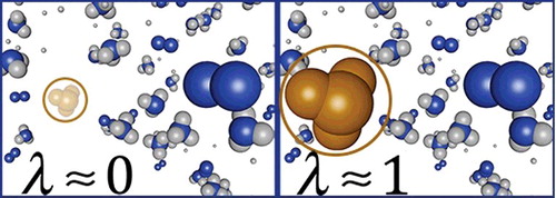The partial molar volume of component A equals (5) A detailed derivation of Equations (3)–(5) is provided in the Supporting Information (Online). Although Equations (3)–(5) are correct, their application is rather limited because of the inefficient sampling of the WTPI method at high densities. Ensemble averages computed using the WTPI method strongly depend on the spontaneous occurrence of cavities large enough to accommodate the test molecule. These spontaneous cavities occur very rarely at high densities which renders the WTPI method essentially inefficient. To circumvent sampling problems of the WTPI method, the CFCMC technique is used to compute the ensemble averages of Equations (3)–(5) without relying on test particle insertions/removals. An expanded version of the conventional NPT ensemble is introduced by adding a so-called fractional molecule (in sharp contrast to the other molecules which are denoted by ‘whole molecules’ throughout this paper). The interaction potential of the fractional molecule is scaled with a coupling parameter λ_A ∈ [0, 1]. λ = 0 means that the fractional molecule has no interactions with the surrounding whole molecules, and therefore it acts essentially as an ideal gas molecule. At λ = 1, interactions of the fractional molecule with the surrounding molecules are fully developed, and the fractional molecule has the same interaction as a whole molecule of the same component. Implementation details regarding the scaling of the interaction potential of fractional molecules are explained in our previous work [23,36,43]. The partition function of the NPT ensemble of a multicomponent mixture of S monoatomic components expanded with a fractional molecule of component A equals [23,43] (6) where Q _CFCNPT is the partition function of the mixture in the continuous fractional component NPT (CFCNPT) ensemble, N is the total number of whole molecules in the system (so not including fractional molecules), Λ _i is the de Broglie thermal wavelength of component i, s are the scaled coordinates of molecules in the system, U is the total interaction potential of whole molecules, and is the scaled interaction potential of the fractional molecule of component A with the whole molecules [39,40,43,43]. λ_A ∈ [0, 1] is the coupling parameter for the interactions of the fractional molecule with the surrounding molecules. The partition function of Equation (6(6) ) can be extended to mixtures of polyatomic molecules by simply multiplying it by the ideal gas partition function of each polyatomic molecule (excluding the translational part) [13,22,72]. This changes only the reference state or the ideal gas contribution of the partial molar properties and not the excess part [3,22,72]. In the Supporting Information (Online), it is shown that the expression for the chemical potential of component A in CFCNPT simulations equals (7) The brackets ⟨⋅⋅⋅⟩_CFCNPT denote an ensemble average in the CFCNPT ensemble. The second term on the right-hand side of Equation (7(7) ) is the excess part of the chemical potential of component A, and it is related to the probability distribution of λ [23]. p(λ_A↑1) is the probability of λ_A approaching 1 and p(λ_A↓0) is the probability of λ_A approaching zero. In the Supporting Information (Online), it is shown that Equations (3(3) ) and (7(7) ) yield identical results.

In the Supporting Information (Online), it is shown that the partial molar enthalpy of component A can be computed in the CFCNPT ensemble using (8) where ⟨H(λ_A↑1)⟩_CFCNPT is the ensemble average enthalpy of the system in the limit at which λ_A approaches one; ⟨H/V (λ_A↓0)⟩_CFCNPT is the ensemble average of the ratio between total enthalpy and the volume of the system in the limit at which λ_A approaches zero. In the Supporting Information (Online), it is shown that Equations (8(8) ) and (4(4) ) yield identical results.

The expression for the partial molar volume of component A in the CFCNPT ensemble equals (9) where ⟨V(λ_A↑1)⟩_CFCNPT is the ensemble average of volume when λ_A approaches one, and ⟨1/V (λ_A↓0)⟩_CFCNPT is the ensemble average of the inverse volume when λ_A approaches zero. In the Supporting Information (Online), it is shown that the computed ensemble average of Equation 9(9) is equal to that computed in the conventional NPT ensemble (Equation (5(5) )). Furthermore, it is shown that the partial molar volume of an ideal gas molecule obtained from Equations (5(5) ) and (9(9) ) results in RT/P (as expected). Using Equations (7)–(9), one can compute the chemical potential, partial molar excess enthalpy, and partial molar volume of a component in a single simulation without relying on the WTPI method or identity changes. A potential drawback of using Equations (8(8) ) and (9(9) ) is that the partial molar (excess) properties are obtained by subtracting two large numbers (at λ = 1 and at λ = 0) with a (relatively) small difference. This may induce large error bars, similar to the ND method explained earlier. In Section 3, it is explained how this can be avoided.

The partial molar excess enthalpy of component A in a mixture can also be computed using EoS modelling. In this paper, partial molar excess enthalpies and partial molar volumes of NH₃, N₂ and H₂ are computed using the PR EoS [73,74] and the PC-SAFT EoS [65,66,75–77]. Details about PR EoS and PC-SAFT EoS are provided in Section 5 of the Supporting Information (Online). The expression for the partial molar enthalpy of component A, relative to the standard reference state, equals [2] (10) where T _ref and P _ref are the standard reference state temperature and pressure defined at 298 K and 1 bar, respectively. h° _{f, A} is the formation enthalpy of component A at the standard reference state (T _ref, P _ref), which can be found in the literature [2,78,79]. The second term on the right-hand side of Equation (10(10) ) is associated with the enthalpy difference at (T, P _ref) at constant composition relative to the reference state. The last term on the right-hand side of Equation (10(10) ) is associated with the excess enthalpy difference between states (T, P) and (T, P _ref). This accounts for departure from ideal gas behaviour relative to the standard reference pressure [2]. can be obtained from molecular simulation (Equations (8(8) ) and (9(9) )), EoS modelling, or the literature. At high temperatures and a pressure of 1 bar, is considered to be zero (ideal gas behaviour). The reaction enthalpy of the Haber–Bosch process (per mole of N₂) at state (T, P) is calculated using (11)

3. Simulation details

In CFCNPT ensemble simulations, beside thermalisation trial moves [22] (volume changes, translations, rotations, etc.), three additional trial moves involving the fractional molecule were used to facilitate the gradual insertion/removal of molecules during the simulation: (1) Changes in λ: the coupling parameter λ is changed while keeping the positions of all molecules including the fractional molecule constant [43]. For changes in λ, it is required that λ is confined to the interval [0, 1] [23,43]. (2) Reinsertions: the fractional molecule is reinserted at a randomly selected position while keeping the positions of all the whole molecules and the value of λ constant [43]. (3) Identity changes: the fractional molecule is changed into a whole molecule of the same component, and a randomly selected whole molecule of the same component is changed into a fractional molecule while keeping the value of λ constant [43]. These trial moves are accepted or rejected based on Metropolis acceptance rules (and automatically rejected when the new value of λ is outside the interval [0, 1]) [22]. It is efficient to combine trial moves (2) and (3) into a single hybrid trial move, as trial move (2) has a high acceptance probability only at low values of λ, and trial move (3) has a high acceptance probability only at high values of λ. In this hybrid trial move, trial move (2) is only selected at low values of λ, and trial move (3) is only selected at high values of λ. This avoids the situations in which trial moves with a very low acceptance probability are selected. Since the value of λ does not change during this hybrid trial move, the probabilities of selecting this trial move and the reverse trial move are identical, and therefore the condition of detailed balance is not violated [22,43]. In practice, one uses a switching point at λ = λ _s to select a trial move of either type (2) or type (3). To facilitate the sampling of λ, a weight function (W(λ)) was used to ensure that the sampled probability of λ is flat [39,40]. In all simulations, maximum molecule displacements, maximum rotations, and maximum volume changes were adjusted to achieve on average 50% acceptance. By attempting a large number of trial moves of types (1), (2), and (3), one can significantly reduce the statistical errors of the computed partial molar properties (Equations (7)–(9)). We found that the hybrid trial moves significantly improve the sampling and reduce the error bars of the computed partial molar properties.

As a proof of principle, MC simulations were performed to compute the partial molar properties of a binary LJ colour mixture (composition: 50%–50%), both in the conventional NPT ensemble using the WTPI method and in the CFCNPT ensemble. All simulations were carried out at a reduced temperature of T ^* = 2 and reduced pressures between P ^* = 0.1 and P ^* = 9, leading to average reduced densities between ρ^* = 0.052 and ρ^* = 0.880. The binary colour mixture contained 200 LJ molecules. σ and ε were set as units of length and energy, respectively. For convenience, the thermal wavelength Λ was set to unity, and all LJ interactions were truncated and shifted at 2.5σ. In the conventional NPT ensemble, 6 × 10⁶ production cycles were carried out. Each cycle consists of N MC trial moves. Each trial move was selected with the following probabilities: 1% volume changes and 99% translations. To sample partial molar properties of each component, ten trial insertions per cycle were performed. In the CFCNPT ensemble simulations, 50 × 10⁶ production cycles were carried out for the same binary mixture at the same reduced temperature and reduced pressures. Each trial move was selected with the following probabilities: 1% volume changes, 33% translations, 33% λ changes, and 33% hybrid trial moves as described earlier. In these hybrid trial moves, a switching point at λ _s = 0.3 is defined. For λ > λ _s , identity changes are attempted, and otherwise a random reinsertion is attempted.

The equilibrium compositions of the [NH₃, N₂, H₂] mixture at 573 K and at various pressures from 10 to 80 MPa were obtained by performing the reaction ensemble simulations of the Haber–Bosch process as described in our previous work [43]. The computed equilibrium compositions are in excellent agreement with experimental data [46,48,49]. All molecules are rigid, and a combination of LJ and electrostatic interactions is used for the force fields. All force field parameters for NH₃, N₂ and H₂ [80–82], cut-off radii for LJ and electrostatic interactions and mixture compositions at equilibrium conditions [43] are provided in Tables S1 and S2 of the Supporting Information (Online). LJ potentials are truncated but not shifted, and analytic tail corrections are applied [22]. The Wolf method was used for the calculation of the electrostatic interactions [83–85]. For simulation details of the reaction ensemble, the reader is referred to the original paper [43]. Equilibrium compositions were then used to initiate the NPT and CFCNPT simulations of the [NH₃, N₂, H₂] mixture. The equilibrium compositions were also used as input for PR EoS modelling and PC-SAFT EoS modelling. Simulation details corresponding to each method are summarised below:

(a)	CFCNPT ensemble: simulations were carried out to compute partial molar properties of NH3, N2 and H2 at 573 K and eight pressures between P = 10 and 80 MPa. To compute partial molar properties of each component, separate simulations were performed in the CFCNPT ensemble, in which one fractional molecule of that component was added to the system. This was repeated for all eight pressures, leading to a total number of 24 independent simulations. The starting mixture compositions for each pressure are listed in Table S1 of the Supporting Information (Online). At each pressure, six independent simulations were carried out where 2 × 105 equilibration cycles were performed to compute the weight function W(λ) using the Wang–Landau algorithm [86,87]. In each cycle, the number of trial moves equals the number of molecules. Starting with equilibrated configurations and weight functions, 3.2 × 106 production cycles were carried out. This leads to six data points per pressure per component. Trial moves were selected with the following probabilities: 1% volume changes, 35% translations, 30% rotations and 17% changes in λ, and 17% hybrid trial moves. Just as for the simulations of the LJ system, for the two remaining trial moves (reinsertions and identity changes), a switching point at λ s = 0.3 was used. Extrapolation was used to evaluate Equations (7)–(9) at λ = 0 and λ = 1.
(b)	ND method: NPT ensemble simulations of the [NH3, N2, H2] mixture were carried out to compute the partial molar properties of each component at 573 K and a pressure range of P = 10 to 80 MPa. To compute the partial molar properties of NH3, N2 or H2 (component A) at each pressure, NPT ensemble simulations of the mixture were performed by changing the number of the molecules of component A with respect to that of the equilibrium mixture (N A), while keeping the number of all other molecules in mixture constant. Seven mixture compositions were used with N A ± 1, N A, N A ± 3 and N A ± 5 molecules around the composition of the equilibrium mixture. Independent NPT simulations were performed for every mixture composition and pressure to compute the total enthalpy (H) and the volume (V) of the mixture as a function of N A. First-order polynomials were fitted to the H and V as a function of N A. The slopes of these lines were calculated to obtain the partial molar excess enthalpy () and the partial molar volume () of component A, respectively. Each NPT simulation was carried out with 2 × 105 equilibration cycles and 5 × 105 production cycles. In each MC step, N trial moves were selected with the following probabilities: 1% volume changes, 49.5% translation trial moves and 49.5% rotation trial moves.
(c)	EoS modelling: the PC-SAFT and PR EoS were used to the compute partial molar excess enthalpies and partial molar volumes of the mixture at the same temperature and pressure range. The same mixture compositions were used for these calculations. For PC-SAFT EoS modelling, ammonia is treated as an associating molecule with four association sites [77,88]. The binary interaction parameters (BIPs) are set to zero both for the PR EoS and PC-SAFT EoS. For additional details, the reader is referred to the Supporting Information (Online).

4. Results

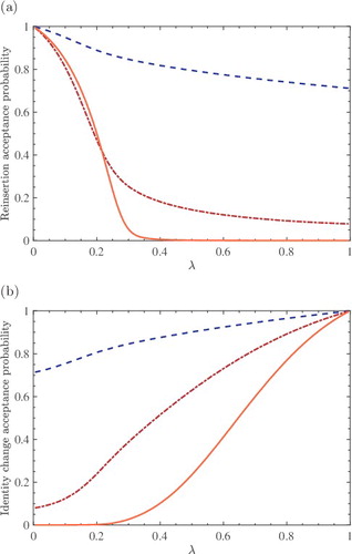
To illustrate the trial moves for the fractional molecule, in Figure 1(a), the acceptance probabilities for reinsertions and identity changes are shown as a function of λ, for the LJ system at ⟨ρ^*⟩ = 0.052, ⟨ρ^*⟩ = 0.433, and ⟨ρ^*⟩ = 0.880. Reinsertion trial moves of fractional molecules are always accepted when λ approaches zero. This is the case for all densities/pressures, which is due to the very limited interactions of the fractional molecule at low values of λ. For the system at the highest reduced density (⟨ρ^*⟩ = 0.880), reinsertion attempts are mostly rejected for λ > 0.3. This is due to overlaps between the reinserted fractional molecule and whole molecules. The acceptance probabilities of attempted identity changes as a function of λ are shown in Figure 1(b). In sharp contrast to reinsertions, molecule exchanges are mostly accepted when the value of λ is close to one. This is expected as a fractional molecule with nearly fully scaled interactions behaves almost as a whole molecule. Therefore, the energy difference associated with this trial move is small at values of λ close to one. For the system with the highest density, identity changes are mostly rejected when λ < 0.3. A whole molecule within an equilibrated system already has favourable interactions with the surrounding molecules. For small values of λ, exchanging a whole molecule with the fractional molecule results in formation of a cavity which has an unfavourable energy. As a result, the energy difference associated with this trial move is high at low values of λ. It can be concluded that defining a switch will ensure a high acceptance probability for the hybrid trial move as explained in Section 3. It is found that the same value can be used for the switching point (λ _s = 0.3) in the simulations of the [NH₃, N₂, H₂] system. We feel that this is a coincidence.

Figure 1. (a) Acceptance probabilities for reinserting and (b) identity changes of the fractional molecule of a binary LJ colour mixture (50%–50%) consisting of 200 molecules at T ^* = 2 and different reduced pressures. In both subfigures: P ^* = 0.1 and ⟨ρ^*⟩_CFCNPT = 0.052 (dashed line), P ^* = 1 and ⟨ρ^*⟩_CFCNPT = 0.433 (dash-dotted line), P ^* = 9 and ⟨ρ^*⟩_CFCNPT = 0.880 (solid line).

To validate our final expressions for the partial molar excess enthalpy and partial molar volume (Equations (8(8) ) and (9(9) )), the values of the partial molar properties obtained using simulations in the CFCNPT ensemble and simulations in the NPT ensemble (as proposed by Frenkel, Ciccotti, and co-workers [14,15]) are compared in Figure 2. The excellent agreement between the results shows that Equations (8(8) ) and (9(9) ) are implemented correctly. For values of λ close to one and zero, the quantities in Equations (8(8) ) and (9(9) ) are well behaved. For a typical example, the reader is referred to Figures S3 and S4 of the Supporting Information (Online). The error introduced by extrapolating is smaller than the error bars from the independent simulations. Computed excess chemical potentials using both methods (Equations (3(3) ) and (7(7) )) are in excellent agreement as well. The raw data of Figure 2 and the excess chemical potentials are listed in Table S3 of the Supporting Information (Online). The partial molar excess enthalpies of the LJ system at a reduced temperature of T ^* = 2 and reduced pressures between P ^* = 0.1 and P ^* = 9 are computed using both methods, and the results are compared in Figure 2(a). At low pressures (low densities), excellent agreement is found, and the error bars are small. In Figure 2(a), it is shown that the values of partial molar excess enthalpies approach zero at low pressures which indicates (and confirms) the ideal gas behaviour. However, there is a clear distinction between the computed partial molar excess enthalpies at high pressures (high densities) using these two methods. The performance of the method proposed by Frenkel, Ciccotti, and co-workers [14,15] strongly depends on the sampling efficiency of the WTPI method, and it is well known that WTPI becomes less efficient at high densities [34,36]. Indeed, the values of partial molar excess enthalpies computed using the WTPI method display scatter as the pressure increases, and the error bars are significantly larger compared to those obtained from CFCNPT simulations. CFCNPT simulations provide better statistics for computing the partial molar excess enthalpies as the density of the system increases, and the magnitude of the error bars remains almost the same for the whole pressure range. Average partial molar volumes computed using both methods are shown in Figure 2(b). Similarly, this comparison shows that computation of the partial molar volumes using the WTPI method at high pressures results in poor statistics. Average partial molar volumes computed using CFCNPT simulations have considerably smaller error bars at high pressures.

Figure 2. (a) Computed partial molar excess enthalpies (Equations (4(4) ) and (8(8) )) and (b) partial molar volumes (Equations (5(5) ) and (9(9) )) of a LJ molecule in a binary colour mixture consisting of 200 molecules (50%–50%) at T ^* = 2, reduced pressures between P ^* = 0.1 and P ^* = 9, and reduced densities ranging from ⟨ρ^*⟩_CFCNPT  = 0.052 to ⟨ρ^*⟩_CFCNPT  = 0.880. For an ideal gas, a horizontal line is expected in (b). In both subfigures: computed properties in the CFCNPT ensemble (triangles), computed properties using the WTPI method in the conventional NPT ensemble (squares) as proposed by Frenkel, Ciccotti, and co-workers [14,15]. Some error bars may be smaller than the symbol size. Raw data are listed in Table S3 of the Supporting Information (Online).

It is instructive to compare the efficiency of the CFCNPT method with the ND method. This was tested for the LJ systems. To compute the partial molar properties using the ND method, two simulations are performed in the NPT ensemble (with N − 1 and N + 1 molecules, respectively). The partial molar properties in the CFCNPT ensemble are obtained by computing the quantities in Equations (8(8) ) and (9(9) ) at λ = 0 and λ = 1 in a single simulation. Essentially, in both methods, the derivatives of Equation (1(1) ) are computed using two data points. This means that to obtain the same accuracy in the computed partial molar properties, a single simulation performed in the CFCNPT ensemble inevitably needs to be longer than each of the NPT simulations. We have verified numerically that the error bars are very similar for both methods for a given amount of CPU time (data not provided here). The advantage of the CFCMC approach is that one can compute the excess chemical potential from the same simulation (Equation (7(7) )).

In Figure 3, the partial molar excess enthalpies and the partial molar volumes of NH₃ are plotted as a function of pressure. The raw data with error bars are listed in Table S4 in the Supporting Information (Online). The results are presented from the four methods discussed in Section 3, namely the PR EoS modelling, the PC-SAFT EoS modelling, the ND method, and the CFCNPT simulations. Figure 3(a) shows that the results of the CFCNPT ensemble simulations are in excellent agreement with those obtained from the ND method. This is used as an independent check to validate our method for systems other than a LJ system. The values of partial molar excess enthalpies of NH₃ are negative, and they decrease with increasing pressure. Excellent agreement is also found between the results from MC simulations and EoS modelling for pressures up to 50 MPa. At pressures higher than 50 MPa, the results obtained from PR EoS and PC-SAFT EoS deviate slightly from each other (0.88 kJ mol⁻¹ at P = 80 MPa). For pressures between 50 and 80 MPa, computed partial molar excess enthalpies of NH₃ obtained from MC simulations agree better with those obtained from the PR EoS. Computed partial molar volumes of NH₃ using all methods are shown in Figure 3(b). The results from MC simulations and EoS modelling are in excellent agreement for the whole pressure range.

Figure 3. (a) Computed partial molar excess enthalpies of NH₃ and (b) computed partial molar volumes of NH₃ in a equilibrium mixture at 573 K and pressure range of P = 10–80 MPa. The compositions of the mixtures are obtained from equilibrium simulations of the Haber–Bosch reaction using serial Rx/CFC [43], and are listed in Table S1 of the Supporting Information (Online). In both subfigures: computed properties using the PR EoS (solid black line), computed properties using the PC-SAFT (dashed red line), computed properties using the ND method (squares), computed properties in the CFCNPT ensemble (triangles) using Equations (8(8) ) and (9(9) ). Zero BIPs were used for the EoS modelling. Raw data are listed in Table S4 of the Supporting Information (Online).

In Figure 4(a), computed partial molar excess enthalpies of N₂ are shown as a function of pressure. In contrast to NH₃, the values of the partial molar excess enthalpies of N₂ are positive and increase with increasing pressure. In addition, the difference between the PC-SAFT EoS and the PR EoS is more obvious, specifically for pressures higher than 50 MPa. As the pressure increases, better agreement is found between the results obtained from the PC-SAFT EoS and CFCNPT simulations. In Figure 4(b), the computed partial molar volumes of N₂ are plotted as a function of pressure. Overall, very good agreement between all methods is observed. Raw data are listed in Table S5 in the Supporting Information (Online). Computed partial molar excess enthalpies of H₂ increase also with increasing pressure, as shown in Figure 5(a). The results obtained from the PR EoS deviate the most from the other methods. This difference contributes directly to a significant deviation in the calculated reaction enthalpy (Figure 6) using the PR EoS, specifically at high pressures. The partial molar excess enthalpies obtained from MC simulations and PC-SAFT EoS are in excellent agreement for pressures up to 70 MPa. Partial molar volumes of H₂ computed using different methods are in excellent agreement as shown in Figure 5(b). Raw data are listed in Table S6 in the Supporting Information (Online).

Figure 4. (a) Computed partial molar excess enthalpies of N₂ and (b) computed partial molar volumes of N₂ in a equilibrium mixture at 573 K and pressure range of P = 10–80 MPa. The compositions of the mixtures are obtained from equilibrium simulations of the Haber–Bosch reaction using serial Rx/CFC [43], and are listed in Table S1 of the Supporting Information (Online). In both subfigures: computed properties using the PR EoS (solid black line), computed properties using the PC-SAFT (dashed red line), computed properties using the ND method (squares), computed properties in the CFCNPT ensemble (triangles) using Equations (8(8) ) and (9(9) ). Zero BIPs were used for the EoS modelling. Raw data are listed in Table S5 of the Supporting Information (Online).

Figure 5. (a) Computed partial molar excess enthalpies of H₂ and (b) computed partial molar volumes of H₂ in a equilibrium mixture at 573 K and pressure range of P = 10–80 MPa. The compositions of the mixtures are obtained from equilibrium simulations of the Haber–Bosch reaction using serial Rx/CFC [43], and are listed in Table S1 of the Supporting Information (Online). In both subfigures: computed properties using the PR EoS (solid black line), computed properties using the PC-SAFT (dashed red line), computed properties using the ND method (squares), computed properties in the CFCNPT ensemble (triangles) using Equations (8(8) ) and (9(9) ). Zero BIPs were used for the EoS modelling. Raw data are listed in Table S6 of the Supporting Information (Online).

Figure 6. Computed reaction enthalpy of the Haber–Bosch process per mole of N₂ at 573 K and pressure range of P = 10–80 MPa. The arrow on the left indicates the value of the reaction enthalpy at standard reference pressure (P _ref = 1 bar). The compositions of the mixtures are obtained from equilibrium simulations of the Haber–Bosch reaction using serial Rx/CFC [43]. Different methods used to compute enthalpy of reaction: PR EoS (solid line). PC-SAFT (dashed red line), ND method (squares), CFCNPT ensemble (blue triangles). Zero BIPs were used for the EoS modelling. Raw data are listed in Table S12 of the Supporting Information (Online).

Excess chemical potentials of NH₃, N₂ and H₂ are computed using EoS modelling, CFCNPT simulations, and the results are compared to those obtained from serial Rx/CFC simulations [43] in Figures S5–S7 in the Supporting Information (Online). Raw data are listed in Tables S7–S9 of the Supporting Information (Online). Computed excess chemical potentials using the different methods are within 1 kJ mol⁻¹.

Our results from the PR EoS modelling were obtained using zero BIPs, and slight improvement is expected when using non-zero BIPs [89]. The non-zero BIPs for the PR EoS were taken from the Aspen Plus software (version 8.8) [90]. The partial molar excess enthalpies of NH₃, N₂ and N₂ were computed using PR EoS modelling with non-zero BIPs, and the results are presented in Figs. S8–S10 in the Supporting Information (Online). It is shown that the difference between the partial molar excess enthalpies obtained from the PR EoS and MC simulations/PC-SAFT become smaller at low and medium pressures, but only for N₂ and H₂. At high pressures, large differences between the results obtained from the PR EoS (using non-zero BIPs) and the other methods remain an issue. No changes were observed for the computed partial molar volumes of all components, using non-zero BIPs. Using BIPs enhances the performance of the EoS mainly in Vapour Liquid Equilibria (VLE), calculations and not elsewhere [89,91].

The reaction enthalpies of the Haber–Bosch process are computed at temperature of 573 K and a pressure range of P = 10–80 MPa using Equations (11(11) ) and (10(10) ). The formation enthalpies and the ideal gas contributions are obtained from the data provided in Tables S10 and S11 of the Supporting Information (Online). The partial molar enthalpies in Equation (10(10) ) are computed using the four methods discussed in Section 2. The results are shown in Figure 6, and the raw data are compiled in Table S12 of the Supporting Information (Online). The reaction enthalpy of the ammonia synthesis reaction at 573 K and standard reference pressure of P _ref = 1 bar is 102.07 kJ per mole of N₂. This is indicated in Figure 6 as a reference. Excellent agreement is observed between the reaction enthalpies computed using MC simulations and the PC-SAFT EoS for pressures up to 80 MPa. The reaction enthalpy computed using the PR EoS deviates from the other methods as pressure increases (up to 8% at 80 MPa). This is associated with the well-known limitations of cubic EoS. At high pressures, volumetric estimates, fugacity coefficients and other related derivative thermodynamic properties calculated using the PR EoS are known to be inaccurate [6,59,63,64]. Although it is one of the most widely used cubic EoS in industry [92], certain drawbacks are associated with using cubic EoS. A cubic EoS cannot accurately estimate the properties of a fluid for a full temperature and pressure range. Moreover, the density dependency of the co-volume term is not known, and many different modifications of the attractive term have been proposed in the literature [59,93]. In contrast to cubic EoS, the PC-SAFT EoS is more physically based and takes into account association interactions [67]. Therefore, for associating mixtures (including the mixture studied in this work), the results from PR EoS modelling are expected to be less accurate compared to those obtained from the PC-SAFT EoS modelling and molecular simulations, especially at high pressures [94].

In Figure 6, it is shown that the contributions of the partial molar excess enthalpies to the reaction enthalpy of the Haber–Bosch process become significant at high pressures. Not including the contribution of the partial molar excess enthalpies results in differences of 24%–64% relative to the reaction enthalpy at the reference pressure, in the pressure range of 30–80 MPa. From Table S1, one can observe that at chemical equilibrium, the mole fraction of NH₃ increases when the pressure increases. As NH₃ molecules show association behaviour [62], this results in favourable NH₃–NH₃ interactions. This is reflected by the negative partial molar excess enthalpy of NH₃ at high pressures (see Figure 3). In sharp contrast to NH₃, the N₂–N₂ and H₂–H₂ interactions become less favourable at high pressures as indicated by a positive partial molar excess enthalpy (see Figures 4 and 5). The net result of the pressure behaviour of the partial molar excess enthalpies is that the reaction enthalpy becomes more exothermic at high pressures.

Instead of running three different simulations for the equilibrium mixture, (each with a single fractional molecule of a different type), it is possible to run a single simulation with three fractional molecules at the same time (one of each component). For sufficiently large systems, the fractional molecules do not influence each other, and the structure of the fluid is not disturbed by the presence of the fractional molecules [95]. Therefore, one may compute the partial molar properties of all components in a single CFCNPT simulation using the same method explained in Section 2. The drawback is that more production cycles are needed to obtain results with the same accuracy. More cycles are needed because the number of trial moves related to the coupling parameter are now distributed between three fractional molecules, instead of one. In Table S13 of the Supporting Information (Online), a comparison is made between this procedure and three separate simulations for the equilibrium mixture at P = 50 MPa. Good agreement is found between both methods.

5. Conclusions

An alternative method is presented to compute partial molar excess enthalpies and partial molar volumes in the NPT ensemble combined with CFCNPT. To compute partial molar properties of component A in a mixture, the NPT ensemble of the mixture is expanded with a fractional molecule of type A. Computation of partial molar properties in the CFCNPT ensemble does not have the drawbacks of Widom-like test particle methods, since particle insertions/removals take place in a gradual manner. Three additional trial moves associated with the fractional molecule are introduced: (1) changing the coupling parameter of the fractional molecule (λ), (2) reinsertion of the fractional molecule at a randomly selected position, (3) changing the identity of the fractional molecule with a randomly selected molecule of the same type. The latter two trial moves can be efficiently combined into a hybrid trial move which significantly enhances the sampling of partial molar properties. As a proof of principle, this method is compared to the original method of Frenkel, Ciccotti, and co-workers [14,15] for a binary LJ colour mixture at constant composition and different conditions. Partial molar properties obtained using both methods are in excellent agreement. Our method is also applied to an industrially relevant system: mixtures of NH₃, N₂ and H₂ at chemical equilibrium. We also compared our method to the ND method. This provides an independent check for the results obtained from CFCNPT simulations. Excellent agreement is found between the results obtained from the ND method and the CFCNPT ensemble simulations. It would be interesting to investigate how the method works for associating large molecules with complex internal degrees of freedom and strong intramolecular interactions. For such systems, conformations with λ = 0 and λ = 1 will be very different. The PR EoS and PC-SAFT EoS are also used to compute the partial molar properties of NH₃, N₂ and H₂ at the same mixture compositions and conditions. Excellent agreement was found between the results obtained from the molecular simulations and the PC-SAFT EoS modelling. The results obtained from the PR EoS deviate from the other methods at high pressures. It is shown that the contribution of the partial molar enthalpies in calculating the reaction enthalpy of the Haber–Bosch process is significant at high pressures (up to 64% at a pressure of 80 MPa, relative to the reaction enthalpy at a pressure of 1 bar). It is observed that at high pressures, the contribution of the partial molar excess enthalpies is not negligible for this process, leading to a more exothermic process at high pressures. It is expected that partial molar properties at high pressures are more accurate using a physically based EoS such as PC-SAFT or advanced MC techniques compared to a cubic EoS. However, cubic EoS are widely used to study other industrially important applications due to their simplicity; for example, the methanol synthesis reaction which is carried out at elevated pressures up to 10 MPa  [19,60,61]. To better understand these processes, it is important to use methods which can accurately model the nonideal behaviour of the system.

Acknowledgments

This work was sponsored by NWO Exacte Wetenschappen (Physical Sciences) for the use of supercomputer facilities, with financial support from the Nederlandse Organisatie voor Wetenschappelijk Onderzoek (Netherlands Organization for Scientific Research, NWO). The authors also gratefully acknowledge the financial support from Shell Global Solutions B.V., and the Netherlands Research Council for Chemical Sciences (NWO/CW) through a VICI grant (Thijs J. H. Vlugt).

Disclosure statement

No potential conflict of interest was reported by the authors.

Additional information

Funding

NWO Exacte Wetenschappen (Physical Sciences), with financial support from the Nederlandse Organisatie voor Wetenschappelijk Onderzoek (Netherlands Organization for Scientific Research, NWO); Shell Global Solutions B.V.; and the Netherlands Research Council for Chemical Sciences (NWO/CW) through a VICI grant (Thijs J. H. Vlugt).

References

- S.I. Sandler , Chemical, Biochemical, and Engineering Thermodynamics , 4th ed. (John Wiley & Sons, Hoboken, NJ, USA, 2006).
- M.J. Moran and H.N. Shapiro , Fundamentals of Engineering Thermodynamics , 5th ed. (John Wiley & Sons, West Sussex, England, 2006).
- S.K. Schnell , P. Englebienne , J.M. Simon , P. Krüger , S.P. Balaji , S. Kjelstrup , D. Bedeaux , A. Bardow , and T.J.H. Vlugt , Chem. Phys. Lett. 582 , 154 (2013). doi:10.1016/j.cplett.2013.07.043
- R.A. Alberty , Thermodynamics of Biochemical Reactions , 1st ed. (John Wiley & Sons, Hoboken, NJ, USA, 2005).
- T. Engel and P.J. Reid , Thermodynamics, Statistical Thermodynamics, & Kinetics , 3rd ed. (Prentice Hall, Upper Saddle River, NJ, USA, 2010).
- B.E. Poling , J.M. Prausnitz , and J.P. O’Connell , The Properties of Gases and Liquids , 5th ed. (McGraw-Hill, New York, USA, 2001).
- A. Podgoršek , J. Jacquemin , A. Pádua , and M. Costa Gomes , Chem. Rev. 116 , 6075 (2016).
- D. Almantariotis , O. Fandio , J.Y. Coxam , and M.C. Gomes , Int. J. Greenhouse Gas Control 10 , 329 (2012). doi:10.1016/j.ijggc.2012.06.018
- M.B. Shiflett , B.A. Elliott , S.R. Lustig , S. Sabesan , M.S. Kelkar , and A. Yokozeki , Chem. Phys. Chem. 13 , 1806 (2012). doi:10.1002/cphc.201200023
- D.S. Firaha , O. Hollczki , and B. Kirchner , Angew. Chem. Int. Ed. 54 , 7805 (2015). doi:10.1002/anie.201502296
- B. Zhang , A.C.T. van Duin , and J.K. Johnson , J. Phys. Chem. B 118 , 12008 (2014). doi:10.1021/jp5054277
- S.P., Šerbanović , B.D. Djordjević , and D.K. Grozdanić , Fluid Phase Equilib. 57 , 47 (1990).
- S.P. Balaji , S. Gangarapu , M. Ramdin , A. Torres-Knoop , H. Zuilhof , E.L. Goetheer , D. Dubbeldam , and T.J.H. Vlugt , J. Chem. Theory Comput. 11 , 2661 (2015). doi:10.1021/acs.jctc.5b00160
- P. Sindzingre , G. Ciccotti , C. Massobrio , and D. Frenkel , Chem. Phys. Lett. 136 , 35 (1987). doi:10.1016/0009-2614(87)87294-9
- P. Sindzingre , C. Massobrio , G. Ciccotti , and D. Frenkel , Chem. Phys. 129 , 213 (1989). doi:10.1016/0301-0104(89)80007-2
- I.M. Abdulagatov , A.R. Bazaev , E.A. Bazaev , M.B. Saidakhmedova , and A.E. Ramazanova , J. Chem. Eng. Data 43 , 451 (1998). doi:10.1021/je970287o
- I.M. Abdulagatov , A.R. Bazaev , E.A. Bazaev , S.P. Khokhlachev , M.B. Saidakhmedova , and A.E. Ramazanova , J. Solution Chem. 27 , 731 (1998). doi:10.1023/A:1022657607502
- H. Liu and J.P. O’Connell , Ind. Eng. Chem. Res. 37 , 3323 (1998). doi:10.1021/ie970926o
- R. Chang and J.L. Sengers , J. Phys. Chem. 90 , 5921 (1986). doi:10.1021/j100280a093
- M.B. Shiflett and E.J. Maginn , AIChE J. 63 , 4722 (2017). doi:10.1002/aic.15957
- M. Michelsen and J.M. Mollerup , Thermodynamic Models: Fundamental & Computational Aspects , 2nd ed. (Tie-Line Publications, Holte, Denmark, 2007).
- D. Frenkel and B. Smit , Understanding Molecular Simulation: From Algorithms to Applications , 2nd ed. (Academic Press, San Diego, CA, 2002).
- A. Poursaeidesfahani , A. Torres-Knoop , D. Dubbeldam , and T.J.H. Vlugt , J. Chem. Theory Comput. 12 , 1481 (2016). doi:10.1021/acs.jctc.5b01230
- B. Smit and D. Frenkel , Mol. Phys. 68 , 951 (1989). doi:10.1080/00268978900102651
- S.K. Schnell , R. Skorpa , D. Bedeaux , S. Kjelstrup , T.J.H. Vlugt , and J.M. Simon , J. Chem. Phys. 141 , 144501 (2014). doi:10.1063/1.4896939
- S.M. Walas , Phase Equilibria in Chemical Engineering , 1st ed. (Butterworth-Heinemann, Watham, MA, USA, 1985).
- J.G. Kirkwood and F.P. Buff , J. Chem. Phys. 19 , 774 (1951). doi:10.1063/1.1748352
- P. Krüger , S.K. Schnell , D. Bedeaux , S. Kjelstrup , T.J.H. Vlugt , and J.M. Simon , J. Phys. Chem. Lett. 4 , 235 (2012).
- N. Dawass , P. Krüger , J.M. Simon , and T.J.H. Vlugt , Mol. Phys. ( in press). doi:10.1080/00268976.2018.1434908.
- A.Y. Ben-Naim , Statistical Thermodynamics for Chemists and Biochemists , 1st ed. (Springer Science & Business Media, New York, USA, 1992). doi:10.1007/978-1-4757-1598-9
- B. Widom , J. Stat. Phys. 19 , 563 (1978). doi:10.1007/BF01011768
- K.B. Daly , J.B. Benziger , P.G. Debenedetti , and A.Z. Panagiotopoulos , Comput. Phys. Commun. 183 , 2054 (2012). doi:10.1016/j.cpc.2012.05.006
- C.H. Bennett , J. Comput. Phys. 22 , 245 (1976). doi:10.1016/0021-9991(76)90078-4
- D.A. Kofke and P.T. Cummings , Mol. Phys. 92 , 973 (1997). doi:10.1080/002689797169600
- I. Nezbeda and J. Kolafa , Mol. Simul. 5 , 391 (1991). doi:10.1080/08927029108022424
- A. Rahbari , A. Poursaeidesfahani , A. Torres-Knoop , D. Dubbeldam , and T.J.H. Vlugt , Mol. Simul. 44 , 405 (2018). doi:10.1080/08927022.2017.1391385
- N.B. Wilding and M. Müller , J. Chem. Phys. 101 , 4324 (1994). doi:10.1063/1.467482
- F.A. Escobedo and J.J. de Pablo , J. Chem. Phys. 105 , 4391 (1996). doi:10.1063/1.472257
- W. Shi and E.J. Maginn , J. Chem. Theory Comput. 3 , 1451 (2007). doi:10.1021/ct7000039
- W. Shi and E.J. Maginn , J. Comput. Chem. 29 , 2520 (2008). doi:10.1002/jcc.20977
- W. Shi and E.J. Maginn , J. Phys. Chem. B 112 , 16710 (2008). doi:10.1021/jp8075782
- W. Shi and E.J. Maginn , AIChE J. 55 , 2414 (2009). doi:10.1002/aic.11910
- A. Poursaeidesfahani , R. Hens , A. Rahbari , M. Ramdin , D. Dubbeldam , and T.J.H. Vlugt , J. Chem. Theory Comput. 13 , 4452 (2017). doi:10.1021/acs.jctc.7b00092
- J.W. Erisman , M.A. Sutton , J. Galloway , Z. Klimont , and W. Winiwarter , Nat. Geosci. 1 , 636 (2008). doi:10.1038/ngeo325
- L.J. Winchester and B.F. Dodge , AIChE J. 2 , 431 (1956). doi:10.1002/aic.690020403
- M. Lísal , M. Bendová , and W.R. Smith , Fluid Phase Equilib. 235 , 50 (2005).
- X. Peng , W. Wang , and S. Huang , Fluid Phase Equilib. 231 , 138 (2005). doi:10.1016/j.fluid.2005.02.001
- L.J. Gillespie and J.A. Beattie , Phys. Rev. 36 , 743 (1930). doi:10.1103/PhysRev.36.743
- C.H. Turner , J.K. Johnson , and K.E. Gubbins , J. Comput. Phys. 114 , 1851 (2001).
- J.R. Jennings , Catalytic Ammonia Synthesis: Fundamentals and Practice , 1st ed. (Plenum Press, New York, USA, 1991). doi:10.1007/978-1-4757-9592-9
- H. Xiao , A. Valera-Medina , R. Marsh , and P.J. Bowen , Fuel 196 , 344 (2017). doi:10.1016/j.fuel.2017.01.095
- H. Nozari and A. Karabeyoğlu , Fuel 159 , 223 (2015). doi:10.1016/j.fuel.2015.06.075
- H. Xiao , M. Howard , A. Valera-Medina , S. Dooley , and P.J. Bowen , Energy Fuels 30 , 8701 (2016). doi:10.1021/acs.energyfuels.6b01556
- C. Zamfirescu and I. Dincer , J. Power Sources 185 , 459 (2008). doi:10.1016/j.jpowsour.2008.02.097
- C. Zamfirescu and I. Dincer , Fuel Process. Technol. 90 , 729 (2009). doi:10.1016/j.fuproc.2009.02.004
- M. Kitano , Y. Inoue , Y. Yamazaki , F. Hayashi , S. Kanbara , S. Matsuishi , T. Yokoyama , S.W. Kim , M. Hara , and H. Hosono , Nat. Chem. 4 , 934 (2012). doi:10.1038/nchem.1476
- C.J. van der Ham , M.T. Koper , and D.G. Hetterscheid , Chem. Soc. Rev. 43 , 5183 (2014). doi:10.1039/C4CS00085D
- X. Guo , Y. Zhu , and T. Ma , J. Energy Chem. 26 , 1107 (2017). doi:10.1016/j.jechem.2017.09.012
- J.O. Valderrama , Ind. Eng. Chem. Res. 42 , 1603 (2003). doi:10.1021/ie020447b
- G.H. Graaf and J.G. Winkelman , Ind. Eng. Chem. Res. 55 , 5854 (2016). doi:10.1021/acs.iecr.6b00815
- G. Graaf , P. Sijtsema , E. Stamhuis , and G. Joosten , Chem. Eng. Sci. 41 , 2883 (1986). doi:10.1016/0009-2509(86)80019-7
- G.M. Kontogeorgis and G.K. Folas , Thermodynamic Models for Industrial Applications: From Classical and Advanced Mixing Rules to Association Theories , 1st ed. (John Wiley & Sons, Wiltshire, Britain, 2009).
- K.G. Harstad , R.S. Miller , and J. Bellan , AIChE J. 43 , 1605 (1997). doi:10.1002/aic.690430624
- B.S. Jhaveri and G.K. Youngren , SPE Reservoir Eng. 3 , 1033 (1988). doi:10.2118/13118-PA
- J. Gross and G. Sadowski , Ind. Eng. Chem. Res. 40 , 1244 (2001). doi:10.1021/ie0003887
- N.I. Diamantonis and I.G. Economou , Energy Fuels 25 , 3334 (2011). doi:10.1021/ef200387p
- N.I. Diamantonis , G.C. Boulougouris , E. Mansoor , D.M. Tsangaris , and I.G. Economou , Ind. Eng. Chem. Res. 52 , 3933 (2013). doi:10.1021/ie303248q
- H.C. Turner , J.K. Brennan , M. Lisal , W.R. Smith , K.J. Johnson , and K.E. Gubbins , Mol. Simul. 34 , 119–2008).
- W.R. Smith and M. Lísal , Phys. Rev. E 66 , 011104 (2002). doi:10.1103/PhysRevE.66.011104
- B. Widom , J. Chem. Phys. 39 , 2808 (1963). doi:10.1063/1.1734110
- B. Widom , J. Phys. Chem. 86 , 869 (1982). doi:10.1021/j100395a005
- D.A. McQuarrie and J.D. Simon , Physical Chemistry: A Molecular Approach , 1st ed. (University Science Books, Sausalito, CA, 1997).
- C.T. Lin and T.E. Daubert , Ind. Eng. Chem. Process Des. Dev. 19 , 51 (1980). doi:10.1021/i260073a009
- D.Y. Peng and D.B. Robinson , Ind. Eng. Chem. Fundam. 15 , 59 (1976). doi:10.1021/i160057a011
- J.A. Barker and D. Henderson , J. Chem. Phys. 47 , 2856 (1967). doi:10.1063/1.1712308
- J. Gross and G. Sadowski , Ind. Eng. Chem. Res. 41 , 5510 (2002). doi:10.1021/ie010954d
- K. Mejbri and A. Bellagi , Int. J. Ref. 29 , 211 (2006).
- M.W. Chase , J. Curnutt , H. Prophet , R. McDonald , and A. Syverud , J. Phys. Chem. Ref. Data. 4 , 1 (1975). doi:10.1063/1.555517
- M.W. Chase , J. Phys. Chem. Ref. Data 4 , 1 (1998).
- L. Zhang and J.I. Siepmann , Collect. Czech. Chem. Commun. 75 , 577 (2010). doi:10.1135/cccc2009540
- J.J. Potoff and J.I. Siepmann , AIChE J. 47 , 1676 (2001). doi:10.1002/aic.690470719
- C.H. Turner , J.K. Johnson , and K.E. Gubbins , J. Chem. Phys. 114 , 1851 (2001). doi:10.1063/1.1328756
- R. Hens and T.J.H. Vlugt , J. Chem. Eng. Data (in press). doi:10.1021/acs.jced.7b00839.
- D. Wolf , Phys. Rev. Lett. 68 , 3315 (1992). doi:10.1103/PhysRevLett.68.3315
- D. Wolf , P. Keblinski , S.R. Phillpot , and J. Eggebrecht , J. Chem. Phys. 110 , 8254 (1999). doi:10.1063/1.478738
- F. Wang and D.P. Landau , Phys. Rev. Lett. 86 , 2050 (2001). doi:10.1103/PhysRevLett.86.2050
- P. Poulain , F. Calvo , R. Antoine , M. Broyer , and P. Dugourd , Phys. Rev. E 73 , 056704 (2006). doi:10.1103/PhysRevE.73.056704
- Aspen Polymer Plus V7.1 Database (Aspen Technology Inc., Bedford, MA, USA).
- A.M. Abudour , S.A. Mohammad , R.L. Robinson , Jr, and K.A. Gasem , Fluid Phase Equilib. 383 , 156 (2014). doi:10.1016/j.fluid.2014.10.006
- Aspen Plus V8.8 Database (Aspen Technology Inc., Bedford, MA, USA).
- A.M. Abudour , S.A. Mohammad , R.L. Robinson , Jr, and K.A. Gasem , Fluid Phase Equilib. 434 , 130 (2017). doi:10.1016/j.fluid.2016.11.019
- C.H. Twu , J.E. Coon , and D. Bluck , Ind. Eng. Chem. Res. 37 , 1580 (1998). doi:10.1021/ie9706424
- Y.S. Wei and R.J. Sadus , AIChE J. 46 , 169 (2000). doi:10.1002/aic.690460119
- S.E. Meragawi , N.I. Diamantonis , I.N. Tsimpanogiannis , and I.G. Economou , Fluid Phase Equilib. 413 (Supplement C), 209 (2016). doi:10.1016/j.fluid.2015.12.003
- A. Poursaeidesfahani , A. Rahbari , A. Torres-Knoop , D. Dubbeldam , and T.J.H. Vlugt , Mol. Simul. 43 , 189 (2017). doi:10.1080/08927022.2016.1244607