Charge migration engineered by localisation: electron-nuclear dynamics in polyenes and glycine

ABSTRACT

We demonstrate that charge migration can be ‘engineered’ in arbitrary molecular systems if a single localised orbital – that diabatically follows nuclear displacements – is ionised. Specifically, we describe the use of natural bonding orbitals in Complete Active Space Configuration Interaction (CASCI) calculations to form cationic states with localised charge, providing consistently well-defined initial conditions across a zero point energy vibrational ensemble of molecular geometries. In Ehrenfest dynamics simulations following localised ionisation of -electrons in model polyenes (hexatriene and decapentaene) and -electrons in glycine, oscillatory charge migration can be observed for several femtoseconds before dephasing. Including nuclear motion leads to slower dephasing compared to fixed-geometry electron-only dynamics results. For future work, we discuss the possibility of designing laser pulses that would lead to charge migration that is experimentally observable, based on the proposed diabatic orbital approach.

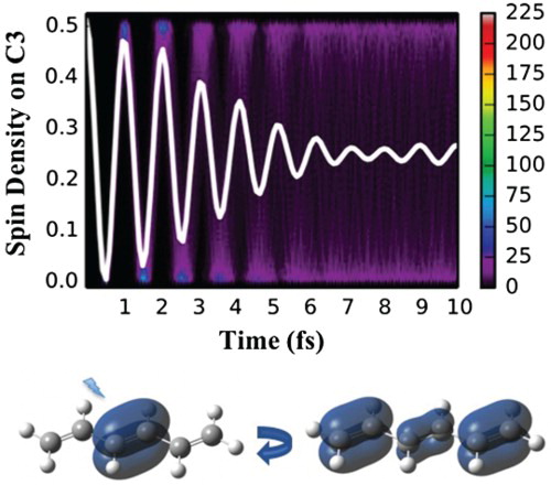
GRAPHICAL ABSTRACT

KEYWORDS:

• Ehrenfest method
• coupled electron-nuclear dynamics
• charge migration
• localised orbitals

I. Introduction

With the rapid development of ultrafast imaging techniques, which are currently reaching time resolution of a few attoseconds (10⁻¹⁸ s), tracking electron dynamics in atoms and molecules becomes a realistic possibility [1–7]. Since any spectroscopic measurement involves interaction of matter with a light beam, atoms and molecular systems undergo energy transitions that, depending on the incident pulse frequency, may lead to changes in their electronic structure. If a laser pulse possesses enough energy, one or more electrons can be emitted, leaving the bound energy states of a system. Pulses having a large spectral bandwidth, such as in attosecond spectroscopy, may populate several cationic eigenstates coherently, forming an electronic wave packet, with the specific composition depending on the shape of the incident pulse. The system thereby finds itself in a non-stationary state that starts evolving with time. If for example photoionisation of a molecule results in a linear superposition of two states, each composed of two single-hole configurations, time evolution of the corresponding wave packet can result in a hole moving (‘beating’) between different parts of the molecule. Such processes are called charge migration. Since photoionisation is often an integral part of spectroscopic measurements being either a result of a probe or both probe and pump pulses, it is important to understand the nature of charge migration for both fundamental and the practical reasons. While in principle the just-ionised cationic system still interacts with the outgoing electron, most electron dynamics computations have ignored this interaction, except in small systems [8], due to the difficulties in accurate description of the electronic continuum. Furthermore, in their recent paper, Martin et al. have shown that such an interaction lasts less than one femtosecond and has a negligible effect on the charge migration following the inner-valence ionisation in glycine [9].

In the recent literature, in attempts to model molecular electronic dynamics in cationic systems, the initial conditions have been mainly constructed from chemical intuition [10–23]. In those studies, the initial wave packet was generally a superposition of two cationic eigenstates, which resulted in a localised charge. This localised charge then evolved in time because of the non-stationary nature of the initial wave function. Such two-state model calculations have revealed some fundamental principles of electron dynamics related to the nature of the electron-nuclear coupling. Specifically, there are two important properties of charge migration that have been observed for different model molecular systems: (a) charge migration is initially (for up to ∼10 fs) mostly unaffected by classical nuclear motion [9,18] and (b) the zero point energy (ZPE) distribution of nuclear geometries (nuclear wave packet width) leads to a fast (usually within 5 fs) decoherence of an averaged signal (shown by both the semi-classical Ehrenfest [20–22] and fully quantum dynamics calculations [23,24]). In the fully quantum picture, quick decoherence is caused by dephasing of the different nuclear wave packet components [23], with the main contribution arising from the low-frequency modes [24]. In the semi-classical picture, since an electronic wave packet oscillation frequency is inversely proportional to the energy gap between the eigenstates involved, sampling over an ensemble of ZPE geometries leads to a broad distribution of oscillation frequencies even for the most rigid systems with well-defined chromophores [21], resulting in the several-femtosecond decoherence rates of the averaged charge migration signal. Still, several full periods can be achieved depending on the molecular structure, which should be enough to detect them experimentally [22]. To the best of our knowledge, such experimental evidence is however still missing, which we attribute to the lack of directed design of excitation pulses, a potential remedy for which we describe below.

The more general approach to electron dynamics following photoionisation involves the construction of an initial electronic wave packet by deriving the electronic eigenstate coefficients from an existing laser pulse shape and from the electronic transition dipole moment matrix elements [3,9,25]. Assuming a single fixed nuclear geometry, let us write a time-dependent electronic wave packet as (1) where represents the electronic eigenstates with the associated energies . The expansion coefficients change during the excitation process but remain constant afterwards. If we now assume a relatively low-intensity pulse, the expansion coefficients at the end of the pulse can be expressed as [9,25,26]: (2) where is the optical excitation pulse in the frequency domain obtained from the experiment. Since the correct definition of includes the outgoing electron, an explicit treatment of the continuum is highly desirable in order to obtain accurate transition probabilities, although approximations such as Dyson orbitals are also employed. Such an approach is however quite limited in its capabilities – it only allows one to model charge migration initiated by the given pulse shape, which may result in nearly no electron dynamics being observed and does not provide any direct route to optimise the pulse [25].

The approach just outlined works both ways. The pulse may be known from the experiment, and so the can be used in theoretical simulations. Alternatively, we may ‘design’ a superposition of states from simulations, and then predict the laser pulse to be used experimentally. In this paper, we suggest investigating this second approach, where one first designs a superposition of eigenstates that would lead to stable electron dynamics from first principles and then reconstructs (at least in a crude way) the pulse that would result in the given superposition of eigenstates and therefore in an experimentally observable charge migration. Here we show how one might design a coherent superposition built from localised states, the first part of the approach outlined above. Below we briefly illustrate how the coherent superposition could in fact be used to predict a laser pulse.

In order to design a superposition of states that would lead to observable electron dynamics, we need to be mindful of the issue of the coupled nuclear dynamics. As we have demonstrated in other work [19–21], it is not the mean-field molecular geometry change that leads to fast decoherence of electron dynamics, but rather the spread of the nuclear wave packet (zero point motion) in the neutral ground state (part of the initial conditions) that causes the issue. If the initial electronic wave packet is chosen to be constructed from the limited number of eigenstates defined in terms of configurations built from delocalised canonical orbitals, then the conditions across the ZPE vibrational wave packet will not in general be unique since the delocalised orbitals will change with the displacement of nuclear geometry. This is particularly true for inner-valence states such as ionised -bonds or -orbitals in a polyene. In contrast, localised orbitals are inherently diabatic and ‘move’ unchanged with the geometry. Defining the initial electronic wave packet in terms of configurations built from such localised orbitals therefore leads to unique initial conditions across the zero point nuclear vibrational wave packet.

To construct localised cationic states, we will use configurations built from natural bonding orbitals (NBO) [27]. NBO are computed as a transformation of the canonical SCF or Kohn–Sham (KS) orbitals that leaves the energy of the neutral ground state unchanged. The occupied NBO represent isolated bonds and lone pairs. The virtual NBO are in general ‘paired’ with the occupied NBO to form localised anti-bonds. Other, more specialised approaches exist to construct diabatic orbitals, such as the one described in the work of Xu et al. [28], but we decided to use NBO due to the simplicity and widespread usage of this localisation method. We will use the term CASCI (Complete Active Space Configuration Interaction) to denote a CI computation containing all the possible cationic states that can arise from a set of NBO with electrons (i.e. just the CI part of CASSCF method). If the NBO are chosen to include only the orbitals doubly occupied in the neutral ground state (with ), and the NBO are built from SCF orbitals, then the eigenstates are just equivalent to the usual Koopmans states [29], but written as a combination of localised states. If the active space includes unoccupied NBO, then one effectively includes polarisation effects in the wave function.

Thus, initiating electron dynamics in a CASCI calculation in the basis of a chosen subset of NBO, just described, one can obtain an initial wave packet representation in terms of the system eigenvectors and their weights ( coefficients in Equation (1)), assuming this subset spans the space close to that of the eigenvectors. One can then simply rewrite Equation (2) in order to obtain an approximate ‘stick’ profile of a model laser pulse: (3)

Such a profile can in principle be fitted to a smooth function representing a pulse shape that can be assumed e.g. in the Gaussian form [26]: (4)

Here, is a pulse parameter related to the spectral bandwidth (and thus pulse duration) and is pulse phase. In this way, one can attempt to design a pulse that would lead to a localised initial wave packet and therefore an observable charge ‘beating’. One needs an estimate for the transition amplitudes in Equation (3), both threshold and to the continuum states, so an explicit treatment of the continuum is required. The related literature especially concerning atomic calculations is vast, but a brief overview of the methods used for molecules is given in [30].

This article is structured as follows. In Section II we describe computational methodology used in the current work. In Sections IIIA and IIIB, we study the two test cases: charge migration in systems of hexatriene and decapentaene and in the space of low-valence orbitals of glycine. In all of these cases, diabatic orbitals are crucial in order to obtain coherent electron dynamics. We expect charge migration designed in this way to be experimentally detectable, although it still decays over a range of rather short lifetimes. The estimated dephasing half-lives are shown to be 4.0 and 4.1 fs for hexatriene and decapentaene, respectively, and 1.7 fs for glycine. We further give a detailed discussion of the nature of observed oscillations depending on the electronic wave packet composition and the effect that nuclear movement has on the dephasing rate. Finally, in Section IV, we provide some further discussion and conclusions.

II. Computational details

All quantum chemical calculations were performed with a development version of Gaussian [31]. Initial reference nuclear geometries were obtained by optimising neutral species at the B3LYP/6-31G* level of theory. To mimic the quantum distribution of the vibrational ground state, frequency calculations were performed at equilibrium structures at the same level of theory, and 500 nuclear geometries and velocities were sampled from the Wigner distribution in the harmonic approximation [32], using the Newton-X program [33]. Single point energy calculations at the same level of theory were then performed for each of the sampled geometries and the resulting KS orbitals were used to generate the full set of NBO individually for each structure. CASCI calculations in the basis of a chosen subset of occupied neutral NBO were then performed for the cationic species (strictly speaking, we were not doing pure CASCI calculations as the core and virtual orbitals were optimised as described below, but we use this name to emphasise that the active orbitals were kept intact and only re-normalised during Ehrenfest dynamics). The number of configuration state functions (CSF) was equal to the number of active NBO and was represented by the single-hole configurations only (we will therefore adopt a notation NBO-CSF(i) in order to indicate the CSF that has all the orbitals doubly occupied with the exception of NBO-i being singly occupied). By performing a CASCI calculation, one effectively obtains an eigenstate decomposition in terms of the NBO basis that can be written as a matrix (see Tables 1–3). Due to it being a unitary matrix (with rows being eigenstates of a Hermitian operator), each column represents a single NBO decomposition in terms of eigenstates and if one defines the initial wave packet as a singly ionised NBO, those columns provide the eigenstate coefficients in Equation (2).

Table 1. Hexatriene CASCI(5,3) eigenstate assignment and decomposition in terms of basis NBO at equilibrium geometry.

Eigenstate	NBO-1	NBO-2	NBO-3	CASCI ΔE, eV	Assignment	OVGF ΔE, eV
1	0.7203	0.4905	−0.4905	0.00	3a’’	0.00
2	0.0000	0.7071	0.7071	2.08	2a’’	2.31
3	0.6937	−0.5093	0.5093	4.08	1a’’	3.79

Notes: Rows represent the eigenstates, while columns contain contributions from a given NBO (see also Figure 1). CASCI and OVGF energy differences with respect to the 3a''  ionisation energy are provided for comparison.

Table 2. Decapentaene CASCI(9,5) eigenstate assignment and decomposition in terms of basis NBO at equilibrium geometry.

Eigenstate	NBO-1	NBO-2	NBO-4	NBO-3	NBO-5	CASCI ΔE, eV	Assignment	OVGF ΔE, eV
1	0.5967	0.5015	−0.5015	−0.2655	0.2655	0.00	3au	0.00
2	0.0000	0.5163	0.5163	0.4832	0.4832	1.16	2bg	1.81
3	0.5666	−0.0290	0.0290	0.5819	−0.5819	2.62	2au	3.17
4	0.0000	−0.4832	−0.4832	0.5163	0.5163	4.02	1bg	4.20
5	0.5682	−0.4977	0.4977	−0.3014	0.3014	5.02	1au	4.80

Notes: Rows represent the eigenstates, while columns contain contributions from a given NBO (see also Figure 1). CASCI and OVGF energy differences with respect to the 3a_u ionisation energy are provided for comparison.

Table 3. Glycine CASCI(15,8) eigenstate assignment and decomposition in terms of basis NBO at equilibrium geometry.

Eigenstate	NBO-1	NBO-2	NBO-3	NBO-4	NBO-5	NBO-6	NBO-7	NBO-8	CASCI ΔE, eV	Assignment	OVGF ΔE, eV
1	−0.1752	0.0004	−0.0048	0.9451	−0.2064	−0.1748	0.0114	−0.0525	0.00	15a'	0.00
2	0.1575	0.4141	0.2857	0.1464	0.7008	−0.2032	−0.4027	−0.0779	3.79	13a'	3.64
3	−0.0161	0.3510	−0.3983	0.1231	0.4062	0.2362	0.6902	0.0746	7.02	11a'/12a'	5.73
4	0.5381	−0.4815	0.0453	0.2593	0.2166	0.5035	−0.0965	0.3155	7.30	12a'/11a'	6.13
5	−0.3125	0.4431	0.0530	0.0060	−0.1978	0.3574	−0.2821	0.6758	12.69	10a'	9.17
6	−0.0687	0.2129	−0.0446	0.0518	−0.1165	0.6695	−0.2347	−0.6545	17.55	9a'	12.23
7	0.5904	0.4260	0.4570	0.0133	−0.4059	−0.0262	0.3084	−0.0186	30.59	7a'
8	−0.4514	−0.2242	0.7376	−0.0056	0.1920	0.2053	0.3497	−0.0259	34.97	6a'

Notes: Rows represent the eigenstates, while columns contain contributions from a given NBO (see also Figure 9). CASCI and OVGF energy differences with respect to the 15a'  ionisation energy are given for comparison.

Correspondingly, in the time-dependent calculations, the initial electronic wave packet was a superposition of all CASCI eigenstates, weighted by the contribution made to them by a chosen single NBO-CSF(i). Such calculations, derivation and implementation details of which have been described previously [17,34], were performed both with and without nuclei moving. The propagation was done in the basis of CSF generated within the chosen active space, so was numerically complete and spanned the whole configuration space.

The general method is as follows. By integrating the time-dependent electronic Schrödinger equation and discretising time, assuming a constant electronic Hamiltonian over a time step, one obtains: (5)

The time-dependent electronic wave function is expanded in the basis of CSF. By gathering the expansion coefficients at time in the vector : (6)

Equation (5) using matrix notation reads as (7)

Thus, in our current implementation, the CI vector is being propagated in discretised steps, with the orbital coefficients remaining constant. (We note that equations of motion for orbital coefficients have been reported for the time-dependent CASSCF method [35].)

The nuclear geometry can be updated, if wanted, at each time step by integrating Newton's equation of motion that for the nuclei reads: (8)

We use the mean-field Ehrenfest (time-dependent) potential expanded to second order in terms of CASSCF energy, gradients and Hessian, computed analytically. One can then choose one of the following options: optimise molecular orbitals at each step, perform a single quadratic step or leave orbitals intact, only allowing for re-orthonormalisation with every change of geometry. Here, we adopted the (arguably more correct) latter approach, only modified to allow for the core-virtual orbital rotations and enabling the active space NBO to follow the nuclear movements diabatically (hence the CASCI name used here). Since neither active orbitals nor expansion coefficients are optimised, we need the full Almlöf and Taylor treatment [36]. Such an approach became possible only recently, with the implementation of the corrected time-dependent Hessian, obtained with the full solution of the coupled-perturbed (CP-MCSCF) equations including all the necessary terms. Details of this implementation will be reported elsewhere.

In order to follow the evolution of the electronic wave function (hole dynamics), we evaluate the time-dependent spin density and partition it onto the atoms using standard Mulliken population analysis [37]. We make use of the spin density calculated in the basis of S² functions recently implemented in the developmental version of Gaussian using the spin-dependent unitary group approach [38]. To quantify the dephasing rate of charge migration, we estimate approximate half-lives of the ensemble average spin density oscillations using a model Gaussian decay formula derived in one of our previous work [19]. Since this formula has been developed for a two-state model, we only apply it to the cases where a single oscillation frequency dominates.

III. Test case systems

A. Polyene charge migration

We begin with an example where the ultimate target is a very long flexible chain of identical chromophores such as a polyene. Ionisation of a localised moiety, say a local C=C bond, results in a state which is obviously not an eigenstate of the cation and electron dynamics thus becomes possible. As previously discussed, the cationic eigenstates are completely delocalised and so there is a priori no obvious coherent superposition of them that might lead to oscillatory charge migration. Furthermore, a state formed from a simple superposition of delocalised states will not retain its diabatic identity over the spread of the ZPE wave packet. We therefore build our localised cationic states from the double bond KS NBO as discussed in Section II.

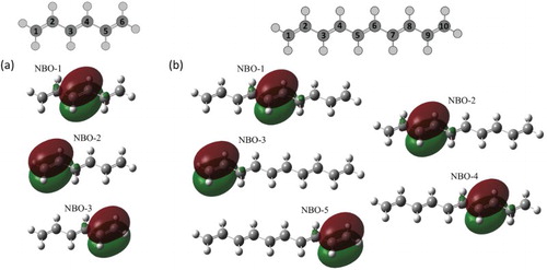
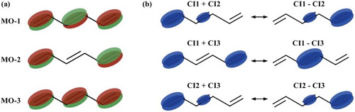
Consistent with the number of double bonds in the chain, the active spaces in the current work are composed of the three and five NBO in cases of hexatriene and decapentaene, respectively (see Figure 1). Those NBO span the full space of system cationic eigenstates for symmetric equilibrium geometries, and the NBO-to-eigenstate transformation matrix obtained by diagonalisation of the CASCI Hamiltonian is therefore exact (see Tables 1 and 2). For the broken-symmetry geometries, due to coupling of - and -orbitals (canonical), this is only true approximately, but it is still a more robust approach than using canonical molecular orbitals (CMO) to define the initial conditions of the electronic wave packet. We performed frozen-geometry electron dynamics calculations as well as Ehrenfest nuclear dynamics for both hexatriene and decapentaene in the full space of the resulting NBO-CSF (CASCI(5,3) and CASCI(9,5), respectively). Both sets of calculations have been initiated by ionising either the central (NBO-1) or one of the distal (NBO-2 for hexatriene and NBO-2 and 3 for decapentaene) orbitals. For both molecules, we performed calculations for ensembles of 500 geometries sampled according to the Wigner distribution. The density functional theory SCF calculations followed by the KS NBO evaluation and CASSCF core and virtual orbitals relaxation have precluded every sampled geometry dynamics run.

Figure 1. Carbon atom numbering and NBO active spaces for (a) hexatriene and (b) decapentaene.

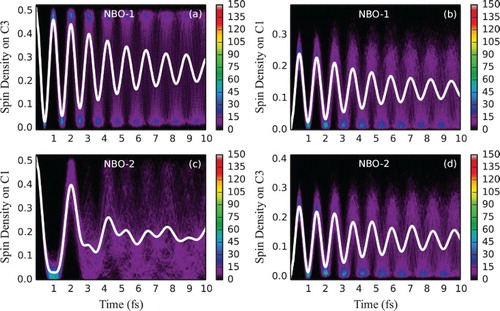
We now discuss hexatriene dynamics. Figure 2 shows the time evolution of spin density for the frozen equilibrium geometry. Following ionisation from NBO-1, an unpaired electron probability density is initially localised on the central bond (equally partitioned by Mulliken analysis to C3 and C4) but is rapidly propagating in both directions up to the distal carbon atoms and back (Figure 2(a)). Averaged over an ensemble, spin density quickly delocalises along the chain due to the differences in the cationic eigenstate energy gaps for different geometries and thus a wide distribution of oscillation frequencies. This can be seen in Figure 3(a,b), depicting time evolution of spin density at one of the central double bond carbon atoms (C3) and one of the distal carbon atoms (C1) (arbitrarily chosen as representative sites of charge migration) for an ensemble of fixed geometries. Starting from the identical spin density at time zero, the ensemble average rapidly dephases, with the estimated half-life of 3.5 fs. Since NBO-1 only contributes to eigenstates 1 and 3 (at least at the symmetric equilibrium geometry, see Table 1), the single average oscillation frequency (with the period of ∼1 fs) observed at both atoms is as expected. A slight re-phasing of the average signal as seen at around 9 fs, not expected for the two-eigenstate mixing case [19], dephases again soon and could be attributed either to an incomplete sampling of the vibrational wave packet or to the fact that for the distorted geometries other eigenstates can mix in (see Supplementary Material for a longer time plot and convergence of the average spin density oscillation with respect to the size of the ensemble).

Figure 2. Snapshots of the spin density evolution following ionisation from (a) NBO-1 and (b) NBO-2 in the hexatriene molecule. Simulation with fixed nuclei, at the equilibrium geometry of the neutral species. Isovalue of 0.002 is used. Lightning bolt symbol designates the ionisation site.

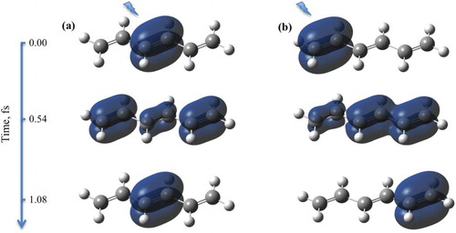
Figure 3. Electron dynamics in hexatriene (with fixed nuclei and sampling): Time evolution of partitioned spin density at C3 and C1 hexatriene atoms, following ionisation from the (a and b) NBO-1 and (c and d) NBO-2 for an ensemble of 500 fixed geometries sampled from the Wigner distribution. For atom labelling and NBO definition, see Figure 1. The side bars indicate the number of sampled trajectories in each pixel of a histogram. Solid white lines indicate spin density averaged over the ensemble.

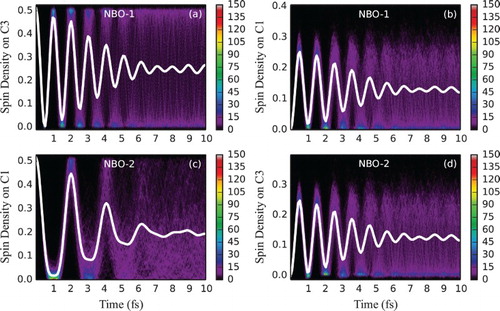
In an alternative setting, dynamics has been initialised by ionising NBO-2. The resulting time evolution of ensemble spin density at atoms C1 and C3 is shown in Figure 3(c,d) (see also Figure 2(b) for the full spin density evolution at the equilibrium geometry). The oscillation period at C3 is approximately half that at C1, and resembles the spin density oscillation at C1 when NBO-1 is ionised (Figure 3b). The two observed frequencies of spin density oscillation, detected at the two carbon atoms, with one being roughly twice the other, can be rationalised using the fact that NBO-2 spans all three eigenstates (see Table 1), with the energy gap between eigenstates 1 and 2 of ∼2 eV being roughly equal to the energy gap between eigenstates 2 and 3 (both therefore contributing to a single slower oscillation frequency of ∼2 fs), each being roughly one half of the energy gap between eigenstates 1 and 3 (producing therefore the twice faster oscillation frequency of ∼1 fs). Time-dependent electronic density can be written in terms of state and transition densities (with the expression being exact at a frozen nuclear geometry) as follows [19]: (9)

The specific oscillation patterns observed at different atoms will depend on their contributions to the transition spin densities between different eigenstates and their expansion coefficients: spin density at atom C3 will change only with , while the other two transition densities will interfere both constructively and destructively with at alternations of approximately 1 fs, with the complete revival of spin density at atom C1 achievable at every 2 fs (see also Figure 4).

Figure 4. Hexatriene: schematic representation of (a) natural molecular orbitals corresponding to the first three CASCI(5,3) eigenstates and (b) density oscillation contributions from each pair of the three CI states. Density at the central double bond (atoms C3 and C4) changes only due to the transition density (middle row) with the frequency defined by the energy gap between states 1 and 3.

Time evolution of spin density at the same atoms for an ensemble of classically moving nuclear geometries (following Ehrenfest equation of motion) is shown in Figure 5. With the overall trend of gradual dephasing maintained, the averaged spin density oscillation is observed for a longer time period as compared to the fixed geometries calculations. While the estimated half-life increases only slightly to 4.0 fs, we note that the oscillation decay is not Gaussian anymore and thus the model function cannot be fitted well enough for the sufficiently long-time period. In fact, the oscillation does not disappear completely within the shown simulated time interval of 10 fs at both C3 and C1 atoms when the central bond (NBO-1) is ionised (Figure 5(a,b)). One can further notice a slight decrease of the oscillation frequency with time. When electron dynamics is initiated by the distal double bond (NBO-2) ionisation, averaged spin density oscillation at C1 becomes somewhat less regular in comparison with the fixed-geometry calculations and dephases at a similar rate while coherence at C3 remains higher (Figure 5(c,d)).

Figure 5. Electron dynamics in hexatriene (with moving nuclei and sampling): Time evolution of partitioned spin density at C3 and C1 hexatriene atoms, following ionisation from the (a and b) NBO-1 and (c and d) NBO-2 for an ensemble of 500 geometries sampled from the Wigner distribution, moving classically. For atom labelling and NBO definition, see Figure 1. The side bars indicate the number of sampled trajectories in each pixel of a histogram. Solid white lines indicate spin density averaged over the ensemble.

The increased half-life seen in simulations with nuclear motion can be explained by the trajectories evolving such that the distribution of geometries becomes narrower, resulting in the distribution of energy differences between states also becoming narrower than in the original ZPE ensemble. In addition, there is a slight decrease in the oscillation frequency, suggesting the now-narrowed distribution of energy differences has also shifted to a lower average value. These assumptions can be confirmed by comparing the standard deviation and mean of the initial energy gap distribution with that of the final distribution. The standard deviation of the energy gap between eigenstates 1 and 2 decreased from 0.22 to 0.18 eV, while the mean decreased from 2.28 to 1.93 eV. Similarly, for the energy gap between eigenstates 2 and 3, the standard deviation decreased from 0.17 to 0.14 eV and the mean from 1.78 to 1.35 eV (see also Figure S3 in the Supplementary Material). A slightly increased irregularity of spin density oscillation at C1 when NBO-2 gets ionised may occur due to the fact that the mean values of the energy gap distributions between the different eigenstates change differently with time, altering the interference pattern and resulting in additional peaks. One should note that there is still more ‘structure’ in the averaged signal in Figure 5(c) compared to Figure 3(c) at a later time, indicating that dephasing is not complete.

In a similar fashion to hexatriene, we performed electron and (electron-nuclear) Ehrenfest dynamics for the 500 sampled geometries of decapentaene, initialised by ionisation of one of the three double bonds: C5–C6 (central, NBO-1), C3–C4 (NBO-2) or C1–C2 (distal, NBO-3) (see Figure 1 for atom and NBO numbering and Figure 6 for the time evolution of spin density at the frozen equilibrium geometry). The resulting ensemble heat maps and averaged spin density time evolution at the C5, C3 and C1 atoms are depicted in Figures 7 and 8 for the fixed and moving nuclei cases, respectively.

Figure 6. Snapshots of the spin density evolution following ionisation from (a) NBO-1, (b) NBO-2 and (c) NBO-3 in the decapentaene molecule. Simulation with fixed nuclei at the equilibrium geometry of the neutral species. Isovalue of 0.002 is used. Lightning bolt symbol designates the ionisation site.

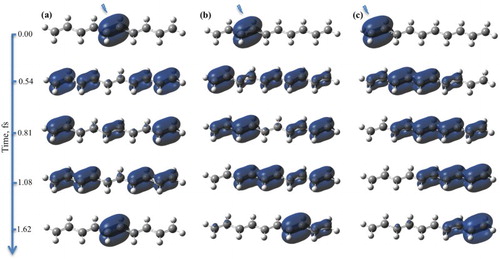
Figure 7. Electron dynamics in decapentaene (with fixed nuclei and sampling): Time evolution of partitioned spin density at C5, C3 and C1 decapentaene atoms, following ionisation from the (a–c) NBO-1, (d–f) NBO-2 and (g–i) NBO-3 for an ensemble of 500 fixed geometries sampled from the Wigner distribution. For atom labelling and NBO definition, see Figure 1. The side bars indicate the number of sampled trajectories in each pixel of a histogram. Solid white lines indicate spin density averaged over the ensemble. Figure 6 can be useful to understand the nature of spin density oscillations (see also discussion in text).

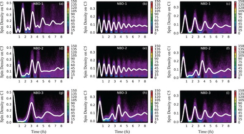
Figure 8. Electron dynamics in decapentaene (with moving nuclei and sampling): Time evolution of partitioned spin density at C5, C3 and C1 decapentaene atoms, following ionisation from (a–c) NBO-1, (d–f) NBO-2 and (g–i) NBO-3 for an ensemble of 500 geometries sampled from the Wigner distribution, moving classically. For atom labelling and NBO definition, see Figure 1. The side bars indicate the number of sampled trajectories in each pixel of a histogram. Solid white lines indicate spin density averaged over the ensemble.

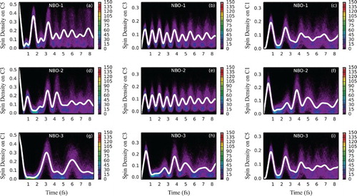
In a longer chain containing five chromophores, charge migration exhibits a more complex pattern due to a larger number of eigenstates contributing to the electronic wave packet. Let us first discuss the frozen-geometry case (Figure 7). When the central double bond (NBO-1) is ionised, eigenstates 1, 3 and 5 get populated (at least at the symmetric equilibrium geometry, see Table 2), amounting roughly to the two energy gaps of 2.5 and 5 eV (with the smaller energy difference contributing twice), giving periods of oscillation of roughly 1.6 and 0.8 fs. Since one period is approximately twice the other, prior to dephasing, we expect to see a full constructive interference at multiples of 1.6 fs and only partially constructive interference at multiples of 0.8 fs. Indeed, larger peaks of spin density at C5 alternate with smaller intermediate peaks at roughly the estimated times (Figure 7(a)). Oscillation patterns at the C3 and C1 atoms are smoother (Figure 7(b,c)), with each plot vividly reflecting only one of the oscillation frequencies. Having fitted the average spin density oscillation at C3 to a model function, the dephasing half-life could be estimated to be 3.6 fs. When other than the central double bond gets ionised (see Figure 7(d–f) for NBO-2 and Figure 7(g–i) for NBO-3 ionisation), more complex patterns can be observed since up to five eigenstates now contribute to the electronic wave packet (see Table 2), resulting in more oscillation frequencies. One can assume that the averaged spin density signals at C3 with NBO-1 being ionised (Figure 7(b)) and at C5 with NBO-2 being ionised (Figure 7(e)) are expected to be the most representative results to be potentially observed in the experiment for an arbitrary-sized polyene due to being associated with non-terminal atoms in a situation when a non-terminal double bond is ionised (with the corresponding periods of oscillation being apparently related to the energy spacing between the lowest and highest-energy eigenstates forming the wave packet).

With the nuclei moving, a similar effect can be observed to that of hexatriene – spin density oscillations are somewhat enhanced (with an estimated half-life of 4.1 fs) with the smaller ‘intermediate’ peaks borrowing intensity from the larger ones, becoming more resolved, but leading to an overall loss of order (see Figure 8). This can be again attributed to the loss of fully constructive and/or destructive interferences due to uneven shifts of different energy gap distributions. Improved coherence can most vividly be observed at C3 and C5 when NBO-1 and NBO-2 are ionised, respectively (Figure 8(b,e)). Here the oscillation frequency is the highest already for the frozen-geometry case, is related to the energy difference between the lowest and highest energy eigenstates and hence is affected to a lesser extent by nuclear movement. The amplitude of those oscillations is however rather low and can be expected to become proportionally smaller with the increase of the size of the molecule.

Overall, for the two polyenes studied here, we have successfully used localised NBO to define initial conditions for charge migration simulation over a ZPE ensemble, providing unique spin density at time zero, i.e. well-defined initial conditions. The average electron dynamics across the ZPE ensemble in decapentaene exhibited a similar dephasing rate to that in hexatriene. However, signal amplitude tends to get lower at the non-terminal atoms in a longer chain of decapentaene (Figure 8(b,e)). One can thus expect to detect experimentally an even weaker charge migration signal when ionising a longer chain of identical chromophores. We further discover that for polyenes, nuclear movement tangibly enhances charge migration coherence.

B. Low-valence glycine charge migration

Inspecting CMO of an arbitrary molecule taken at an isolated nuclear geometry can lead to a suitable choice of a superposition of eigenstates, which would trigger electron dynamics. States that share significant contributions from the same set of configurations are potential candidates to form a time-dependent wave packet. In a simple case, two neighbouring eigenstates would have a 50/50 contribution each from the two configurations carrying a hole in one of the two orbitals (1h/1h mixing). A wave packet composed of those two eigenstates will result in a coherent charge migration between the two contributing orbitals with the period of signal (hole survival probability or spin density) oscillation being inversely proportional to the interstate energy difference.

Among other work, Cooper and Averbukh have described an example of such a low-valence shell charge migration for a glycine molecule at the fixed equilibrium geometry [39] (conformer I according to Kuleff and Cederbaum [40]). Using a single-reference time-dependent ADC(2) electronic structure method, they have shown that the two close-lying cationic excited states are mainly composed of the two configurations with single holes in CMO 11a′ and 12a′. They defined the initial non-stationary state by removing an electron from orbital 11a′ thereby populating both eigenstates. The resulting two-state oscillatory dynamics involved beatings between 11a′- and 12a′-ionised 1h configurations [39].

However, such electron dynamics calculations are not well defined if one allows for sampling the ZPE vibrations. Specifically, glycine orbitals 11a′ and 12a′ have a strong non-local character and are therefore prone to significant deformations with the geometry distortions. In addition, they can couple with other orbitals following symmetry breaking. Thus, the eigenstates of distorted geometries are not consistent with each other (i.e. lose their initial composition in terms of CMO configurations). Of course, we are just saying that the superpositions of eigenstates built from delocalised CMO are far from being diabatic and are thus unsuitable for Ehrenfest computations across the ZPE vibrational sample.

As with polyenes, using NBO that diabatically follow nuclear geometry distortions solves this problem. One technical difficulty is that in multireference calculations one has to resort to a limited subset of orbitals to define an active space. For higher-valence shell calculations, it is usually enough to define a small but complete subset of NBO (e.g. two lone pairs for a higher-valence shell hole-beating or three -bonding orbitals for hexatriene) that would span the full space of eigenstates involved in charge migration. However, if one's aim is to obtain a realistic eigenstate decomposition of a wave packet that would lead to an observable charge migration in a lower-valence shell or across low- and high-valence shells (as in the case of 1h/2h1p charge migration in glycine [41]), one will usually need a much larger subset of NBO that will span the eigenstate space sufficiently.

In an attempt to see if we can model the glycine low-valence 1h/1h charge migration problem described above, we found a subset of 8 KS NBO (shown in Figure 9) to form a representative active space. Intuitive criteria for selection would be to match the CASCI(15,8) eigenstate natural orbitals (NO), obtained at the equilibrium geometry by diagonalising the excited states one-electron density matrices, to the linear combination of the relevant reference SCF CMO from [39]. A more appropriate and unbiased way to assign eigenstates would be by comparing their eigenenergies to the second-order ionisation energies from the contributing SCF CMO. The latter were obtained with the Outer Valence Greens Function (OVGF) method, and while the energies matched very well for the lower values, the error grows very fast for higher energies. Therefore, a visual comparison of CASCI NO to contributing SCF CMO (see Supplementary Material) was still deemed necessary and together with the OVGF energies provided an unbiased assignment of all the cationic eigenstates to the underlying SCF CMO. One should note that while being assigned to ionisation from a single SCF orbital (according to Koopmans theorem), the OVGF ionisation energies account for correlation up to second order, and therefore allow for the 11a′/12a′ configurations mixing in the cationic eigenstates.

Figure 9. Atom numbering and NBO constituting active space for glycine CASCI calculations at the equilibrium geometry.

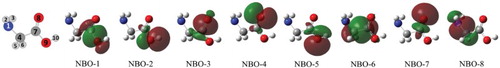
Table 3 shows the CASCI(15,8) eigenstate decomposition (transformation matrix) in terms of the NBO basis (columns) and their assignments based on the NO shapes and OVGF results.

Clearly, none of the NBO contributes exclusively to eigenstates 3 and 4 (mixing 11a′ and 12a′ 1h configurations), spanning other eigenstates to various degrees. Thus, one would not be able to reproduce the Averbukh et al. results initialised by ionisation of a single diabatic orbital, as other eigenstates would mix in. In principle, one could try to use a linear combination of NBO, but this would inevitably lead to non-unique initial conditions across an ensemble, similar to using CMO. However, ionisation from a suitable single NBO spanning two or more eigenstates would still lead to an observable (but different in its nature as compared to the results by Averbukh et al.) low-valence charge migration (i.e. charge migration between two or more bonding orbitals).

An obvious choice was to design charge migration between the two adjacent C–O bonds. The corresponding bonding orbitals are represented by NBO-1 and NBO-3 which, according to Table 3, largely contribute both to eigenstates 6a′ and 7a′ and therefore were expected to generate charge migration when ionised. We decided to initiate electron dynamics by ionising NBO-3.

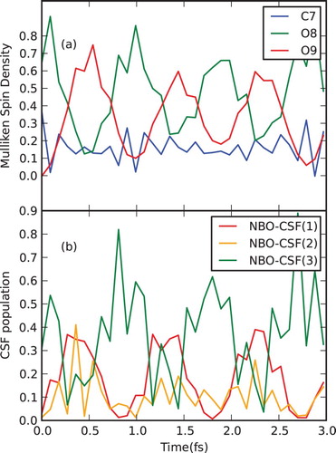
Let us consider the fixed equilibrium geometry first. The spin density evolution at the heavy atoms from the carboxyl group resulting from ionisation of NBO-3 (C7–O8 bond) is given in Figure 10 and Figure 11(a). A regular beating between the carbonyl (O8) and hydroxyl (O9) oxygen atoms is observed, while the value of spin density partitioned at the carbon atom (C7) oscillates only slightly and remains low at all times. The corresponding evolution of the NBO-CSF(1–3) populations is shown in Figure 11(b). Oscillation of NBO-CSF(3) population directly correlates with the spin density evolution at O8, while NBO-CSF(1–2) populations correspond to the O9 spin density, as expected. The NBO-CSF(5,7) also get mixed in, contributing to spin densities of the two oxygen atoms (we omit plotting them here for clarity, providing corresponding data in Supplementary Material). One should note that due to the fact that a given NBO contributes to the whole set of eigenstates, the resulting signal gets very noisy.

Figure 10. Snapshots of the spin density evolution following ionisation of NBO-3 in glycine molecule. Simulation with fixed nuclei, at the equilibrium geometry of the neutral species. Isovalue of 0.02 is used. Lightning bolt symbol designates the ionisation site.

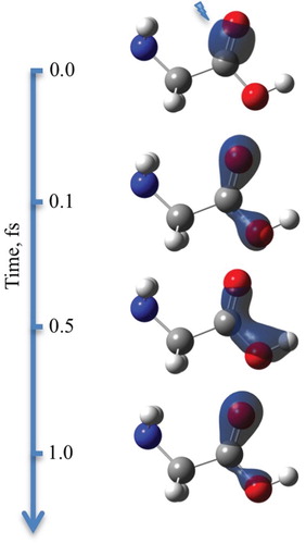
Figure 11. Electron dynamics in glycine (with fixed nuclei): Time evolution of (a) partitioned spin densities at the glycine carboxyl group heavy atoms, and (b) CSF populations, following ionisation from NBO-3. For atom labelling and NBO definition, see Figure 9. Simulation performed at the equilibrium geometry of the neutral species with the nuclei being fixed.

Now let us consider the moving nuclei case. The Ehrenfest dynamics proved to be harder to converge than in the polyene case and nearly one fifth of the sampled trajectories failed due to integration error or developed poor energy conservation (with error >0.001 Hartree). This was mainly associated with extreme elongation of the C7–O9 and O9–H10 bonds as well as development of a very acute C7–O9–H10 angle in some of the trajectories. We thus present here the NBO-3 results for the 403 successful trajectories out of the trial 500 (which is the common sampling size being usually enough to reach convergence of the ensemble average spin density). A more stable propagator may be considered in future for better convergence.

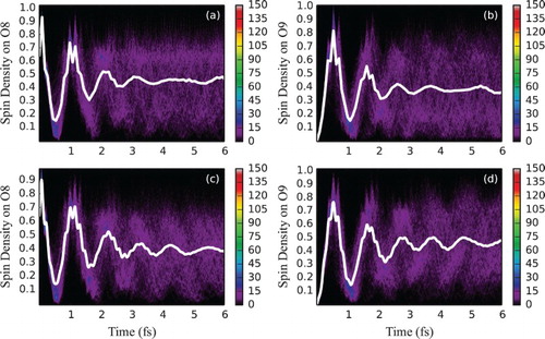
Time evolution of spin density at O8 and O9 for an ensemble of 403 fixed geometries is shown in Figure 12(a,b). The average signals at both atoms dephase relatively fast (with the estimated half-life of 1.4 fs) giving, however, three pronounced oscillation periods before the nearly total delocalisation of spin density over the atoms constituting carboxyl group, predominantly O8 and O9. Results for the converged 403 Ehrenfest trajectories are shown in Figure 12(c,d). Staying very similar to the frozen-geometry case, the average spin density signal is more coherent, with the estimated half-life of 1.7 fs.

Figure 12. Electron dynamics in glycine (with fixed and moving nuclei and sampling): Time evolution of partitioned spin density at O8 and O9 glycine atoms, following ionisation from NBO-3 for an ensemble of 403 geometries sampled from the Wigner distribution with the nuclei (a and b) staying fixed or (c and d) moving classically. For atom labelling and NBO definition, see Figure 9. The side bars indicate the number of sampled trajectories in each pixel of a histogram. Solid white lines indicate spin density averaged over the ensemble.

We have therefore demonstrated the use of localised orbitals in designing observable low-valence charge migration in glycine, allowing us to enforce unique initial conditions over a ZPE ensemble. As in the case of system charge migration in polyenes, we notice an improvement in spin density coherence when allowing nuclei to move. Our results however suggest that ionisation leading to charge migration between chemical bonds may result in bond dissociation, which can in its turn lead to the further signal loss within the first 10 fs.

IV. Discussion and conclusions

In this work, we demonstrate that charge migration can be ‘engineered’ in arbitrary molecular systems if a single localised orbital that diabatically follows nuclear displacements is ionised. By using charge localised diabatic states (here composed of configurations built from NBO), unique initial conditions reflected by the same spin density distribution can be obtained across a ZPE ensemble (i.e. mimicking a ground state vibrational wave packet). This localised state is a superposition of cationic states and the weights of the eigenstates can be computed by CASCI in the basis of localised (NBO) states.

One may ‘reverse engineer’ a pulse that would lead to the charge migration presented here. One can make use of the computed weights to obtain a ‘stick’ profile of a model pulse at the ionisation frequencies by using Equation (3) and then fit the obtained profile to a smooth function such as the one in Equation (4). Such reverse engineering of a specific pulse and its experimental realisation was beyond the scope of the current work, but the authors hope that it can be done in future.

This approach is to be contrasted with the strategy whereby one takes an experimentally generated attosecond pulse and uses it to computationally construct the initial electronic wave packet in order to start the electronic (and optionally coupled nuclear) dynamics (i.e. using Equation (2)). Lara-Astiaso et al. have for example adopted the latter approach in the two recent papers, where an experimental XUV pulse shape is used to explicitly construct the initial wave packet to be propagated both for bound states and in the continuum [9,25].

We presented three molecular test systems: two polyenes and glycine. For such systems, the high flexibility of the carbon backbone would cause the canonical valence orbitals to vary greatly across the ZPE distribution. In both cases, we study the effect of the vibrational wave packet width on the charge migration signal dephasing both with and without moving nuclei. In the first case, slower dephasing has been observed for both polyenes and glycine, suggesting the evolution of an ensemble into a narrower distribution of cationic excited state energy differences. For low-valence charge migration in glycine, eventual bond dissociation has been predicted.

In this work, we used a semi-classical representation of the moving nuclei via ZPE ensembles of independent trajectories and observed relatively long-lived electronic coherences. Ideally, this should be described in a fully quantum manner i.e. by propagating nuclear wave packets [42,43]. However, in our recent paper [23], full quantum dynamic treatment of nuclear motion in polyatomic cations lead to a similar rate of electronic decoherence as compared to the earlier ensemble-based Ehrenfest calculations, except that the nuclear wave packet overlap was in fact found to be responsible for small revivals of coherence. Instead, the main mechanism for decoherence was found to be dephasing, which is exactly what we take into account by using ensembles of independent trajectories. In a recent paper by Arnold et al. [24], where nuclear motion has also been treated quantum mechanically, the electronic coherence was somewhat shorter (not more than 2 fs for polyatomic molecules). Such seeming discrepancies are intriguing and would require further investigation. One should note, however, that different molecules were studied in those two papers (also different from the current work), while decoherence time can be expected to be very molecule-specific. Also, the initial conditions in both papers have been chosen in an ad hoc intuitive fashion, which may have affected the results of fully quantum dynamic calculations, since one of the main ideas of the current work is that the initial conditions may be crucial for electronic coherence.

Acknowledgments

All calculations were run using the Imperial College High Performance Computing service.

Disclosure statement

No potential conflict of interest was reported by the authors.

ORCID

Iakov Polyak http://orcid.org/0000-0002-2894-0657

Andrew J. Jenkins http://orcid.org/0000-0002-1014-5225

Morgane Vacher http://orcid.org/0000-0001-9418-6579

Michael J. Bearpark http://orcid.org/0000-0002-1117-7536

Michael A. Robb http://orcid.org/0000-0003-0478-8301

Additional information

Funding

This work was supported by UK-EPSRC Grant ‘Attosecond Electron Dynamics in Molecular and Condensed Phase Systems’, [grant number EP/I032517/1].

References

- F. Krausz and M. Ivanov, Rev. Mod. Phys. 81, 163 (2009). doi: 10.1103/RevModPhys.81.163.
- G. Sansone, F. Kelkensberg, J.F. Pérez-Torres, F. Morales, M.F. Kling, W. Siu, O. Ghafur, P. Johnsson, M. Swoboda, E. Benedetti, F. Ferrari, F. Lépine, J.L. Sanz-Vicario, S. Zherebtsov, I. Znakovskaya, A. L’Huillier, M.Y. Ivanov, M. Nisoli, F. Martín, and M.J.J. Vrakking, Nature. 465, 763 (2010). doi: 10.1038/nature09084.
- F. Calegari, D. Ayuso, A. Trabattoni, L. Belshaw, S. De Camillis, S. Anumula, F. Frassetto, L. Poletto, A. Palacios, P. Decleva, J.B. Greenwood, F. Martín, and M. Nisoli, Science 346, 336 (2014). doi: 10.1126/science.1254061.
- L. Fang, T. Osipov, B.F. Murphy, A. Rudenko, D. Rolles, V.S. Petrovic, C. Bostedt, J.D. Bozek, P.H. Bucksbaum, and N. Berrah, J. Phys. B. 47, 124006 (2014). doi: 10.1088/0953-4075/47/12/124006.
- F. Lépine, M.Y. Ivanov, and M.J.J. Vrakking, Nature Photonics. 8, 195 (2014). doi:10.1038/NPHOTON.2014.25.
- S.R. Leone, W. McCurdy, J. Burgdörfer, L.S. Cederbaum, Z. Chang, N. Dudovich, J. Feist, C.H. Greene, M. Ivanov, R. Kienberger, U. Keller, M.F. Kling, Z.-H. Loh, T. Pfeifer, A.N. Pfeiffer, R. Santra, K. Schafer, A. Stolow, U. Thumm, and M.J.J. Vrakking, Nature Photonics 8, 162 (2014). doi: 10.1038/nphoton.2014.48.
- F. Calegari, A. Trabattoni, A. Palacios, D. Ayuso, M.C. Castrovilli, J.B. Greenwood, P. Decleva, and F. Martín, J. Phys. B. 49, 1 (2016). doi:10.1088/0953-4075/49/14/142001.
- B. Mignolet, R.D. Levine, and F. Remacle, Phys. Rev. A. 89, 1 (2014). doi: 10.1103/PhysRevA.89.021403.
- M. Lara-Astiaso, D. Ayuso, I. Tavernelli, P. Decleva, A. Palacios, and F. Martín, Faraday Discuss. 194, 41 (2016). doi: 10.1039/c6fd00074f.
- L.S. Cederbaum and J. Zobeley, Chem. Phys. Lett. 307, 205 (1999). doi: 10.1016/S0009-2614(99)00508-4.
- J. Breidbach and L.S. Cederbaum, J. Chem. Phys. 118, 3983 (2003). doi: 10.1063/1.1540618.
- H. Hennig, J. Breidbach, and L.S. Cederbaum, J. Phys. Chem. A. 109, 409 (2005). doi: 10.1021/jp046232s.
- F. Remacle and R.D. Levine, Proc. Natl. Acad. Sci. U.S.A. 103, 6793 (2006). doi: 10.1073/pnas.0601855103.
- A.I. Kuleff and L.S. Cederbaum, J. Phys. B. 47, 124002 (2014). doi: 10.1088/0953-4075/47/12/124002.
- A.I. Kuleff, N.V. Kryzhevoi, M. Pernpointner, and L.S. Cederbaum, Phys. Rev. Lett. 117, 093002 (2016). doi:10.1103/PhysRevLett.117.093002.
- D. Mendive-Tapia, M. Vacher, M.J. Bearpark, and M.A. Robb, J. Chem. Phys. 139, 044110 (2013). doi:10.1063/1.4815914.
- M. Vacher, D. Mendive-Tapia, M.J. Bearpark, and M.A. Robb, Theor. Chem. Acc. 133, 1 (2014). doi:10.1007/s00214-014-1505-6.
- M. Vacher, M.J. Bearpark, and M.A. Robb, J. Chem. Phys. 140, 3 (2014). doi: 10.1063/1.4879516.
- M. Vacher, L. Steinberg, A.J. Jenkins, M.J. Bearpark, and M.A. Robb, Phys. Rev. A. 92, 1 (2015). doi:10.1103/PhysRevA.92.040502.
- A.J. Jenkins, M. Vacher, M.J. Bearpark, and M.A. Robb, J. Chem. Phys. 144, 104110 (2016). doi: 10.1063/1.4943273.
- M. Vacher, F.E.A. Albertani, A.J. Jenkins, I. Polyak, M.J. Bearpark, and M.A. Robb, Faraday Discuss. 194, 95 (2016). doi: 10.1039/c6fd00067c.
- A.J. Jenkins, M. Vacher, R.M. Twidale, M.J. Bearpark, and M.A. Robb, J. Chem. Phys. 145, 164103 (2016). doi: 10.1063/1.4965436.
- M. Vacher, M.J. Bearpark, M.A. Robb, and J.P. Malhado, Phys. Rev. Lett. 118, 083001 (2017). doi:10.1103/PhysRevLett.118.083001.
- C. Arnold, O. Vendrell, and R. Santra, Phys. Rev. A 95, 033425 (2017). doi: 10.1103/PhysRevA.95.033425.
- M. Lara-Astiaso, A. Palacios, P. Decleva, I. Tavernelli, and F. Martín, Chem. Phys. Lett. 683, 357 (2017). doi: 10.1016/j.cplett.2017.05.008.
- A. Kirrander, C. Jungen, and H.H. Fielding, J. Phys. B. 41, 074022 (2008). doi: 10.1088/0953-4075/41/7/074022.
- J.P. Foster and F. Weinhold, J. Am. Chem. Soc. 102, 7211 (1980). doi: 10.1021/ja00544a007.
- X. Xu, K.R. Yang, and D.G. Truhlar, J. Chem. Theory Comput. 9, 3612 (2013). doi: 10.1021/ct400447f.
- T. Koopmans, Physica. 1, 104 (1934). doi:10.1016/S0031-8914(34)90011-2.
- M. Nisoli, P. Decleva, F. Calegari, A. Palacios, and F. Martín, Chem. Rev. (2017). doi:10.1021/acs.chemrev.6b00453.
- M.J. Frisch, G.W. Trucks, H.B. Schlegel, G.E. Scuseria, M.A. Robb, J.R. Cheeseman, G. Scalmani, V. Barone, B. Mennucci, G.A. Petersson, H. Nakatsuji, M. Caricato, X. Li, H.P. Hratchian, J. Bloino, B.G. Janesko, A.F. Izmaylov, A. Marenich, F. Lipparini, G. Zheng, J.L. Sonnenberg, W. Liang, M. Hada, M. Ehara, K. Toyota, R. Fukuda, J. Hasegawa, M. Ishida, T. Nakajima, Y. Honda, O. Kitao, H. Nakai, T. Vreven, K. Throssell, J.A. Montgomery, J. Peralta, J.E.F. Ogliaro, M. Bearpark, J.J. Heyd, E. Brothers, K.N. Kudin, V.N. Staroverov, T. Keith, R. Kobayashi, J. Normand, K. Raghavachari, A. Rendell, J.C. Burant, S.S. Iyengar, J. Tomasi, M. Cossi, N. Rega, J.M. Millam, M. Klene, J.E. Knox, J.B. Cross, V. Bakken, C. Adamo, J. Jaramillo, R. Gomperts, R.E. Stratmann, O. Yazyev, A.J. Austin, R. Cammi, C. Pomelli, J.W. Ochterski, R.L. Martin, K. Morokuma, V.G. Zakrzewski, G.A. Voth, P. Salvador, J.J. Dannenberg, S. Dapprich, P.V. Parandekar, N.J. Mayhall, A.D. Daniels, O. Farkas, J.B. Foresman, J.V. Ortiz, J. Cioslowski, and D.J. Fox, Gaussian Development Version, Revision I.09 (Gaussian, Inc., Wallingford, CT, 2014).
- E. Wigner, Phys. Rev. 40, 749 (1932). doi:10.1103/PhysRev.40.749.
- M. Barbatti, G. Granucci, M. Persico, M. Ruckenbauer, M. Vazdar, M. Eckert-Maksic, and H. Lischka, J. Photochem. Photobiol. A. 190, 228–240 (2007). doi:doi: 10.1016/j.jphotochem.2006.12.008.
- M. Vacher, M.J. Bearpark, and M.A. Robb, Theor. Chem. Acc. 135, 187 (2016). doi:10.1007/s00214-016-1937-2.
- T. Sato and K.L. Ishikawa, Phys. Rev. A. 88, 023402 (2013). doi: 10.1103/PhysRevA.88.023402.
- P.R. Taylor and J. Almlöf, Int. J. Quant. Chem. 27, 743 (1985). doi: 10.1002/qua.560270610.
- R.S. Mulliken, J. Chem. Phys. 23, 1833 (1955). doi:10.1063/1.1740588.
- I. Polyak, M.J. Bearpark, and M.A. Robb, Int. J. Quant. Chem.e25559 (2017). doi: 10.1002/qua.25559.
- B. Cooper and V. Averbukh, Phys. Rev. Lett. 111, 083004 (2013). doi: 10.1103/PhysRevLett.111.083004.
- A.I. Kuleff and L.S. Cederbaum, Chem. Phys. 338, 320 (2007). doi: 10.1016/j.chemphys.2007.04.012.
- B. Cooper, P. Kolorenč, L.J. Frasinski, V. Averbukh, and J.P. Marangos, Faraday Discuss. 171, 93 (2014). doi: 10.1039/C4FD00051J.
- D. Geppert, P. von den Hoff, and R. de Vivie-Riedle, J. Phys. B. 41, 074006 (2008). doi:10.1088/0953-4075/41/7/074006.
- T. Bayer, H. Braun, C. Sarpe, R. Siemering, P. von den Hoff, R. de Vivie-Riedle, T. Baumert, and M. Wollenhaupt, Phys. Rev. Lett. 110, 123003 (2013). doi:10.1103/PhysRevLett.110.123003.