Energetics of molecular motor proteins: could it pay to take a free ride?

ABSTRACT

Molecular motor proteins are used in biological systems to generate directed motion. They consist of one end that can bind to and then move along a filament. The other end can then bind to a cargo that needs transporting and the motor then pulls it along. Here, we consider the energetics of this process allowing for the friction force exerted by the surrounding fluid, given that the process takes place in a confined geometry. In nature, not all motor/cargo complexes are bound to the filament, many are in solution. Here, we address the question of whether this can be energetically favourable given that the unbound complexes will be transported by the flow generated by those that are bound. A simple theory suggests that this is the case and that there exists an optimal coverage of bound complexes. Simulations of a model of this system that includes all the relevant hydrodynamic effects confirm that the assumptions in the theory are valid so long as the coverage of bound complexes is not too low. Using realistic values for the parameters involved yields an optimal coverage that is plausible for the biological systems involved.

GRAPHICAL ABSTRACT

KEYWORDS:

• Motor proteins
• transport
• viscous forces
• energy use

1. Introduction

As anyone who knows Daan knows, paying close attention to what he says at all times is a good idea. You never know when a great idea might be heading your way. That is not to say all Daan's ideas are great (given the huge number that is impossible) but there is a high probability of it, or at worst that it is merely a good or useful one. The title of this article contains a direct quotation from a conversation with Daan. We were talking about transport of material in cells using molecular motors and he mused “could it pay to take a free ride?”. This article is our attempt to answer his question.

Molecular motor proteins are widely used in biological systems to generate directional motion [1]. They are used to generate actual bodily motion, such as muscle contraction, and in cells to move material from one place to another. Here, we are interested in the latter. Directed transport occurs by motor proteins binding to sites on certain semi-stiff ‘track’ filaments that are assemblies of globular proteins with a polarity. They then process in a given direction, determined by the polarity of the track. The exact mechanism by which this occurs is still a matter of debate. However, the consensus is that the motors hydrolyse ATP and undergo a configurational change that moves them along to the next binding site [2,3]. Motor proteins primarily differ in the track to which they bind and in which direction they move once bound to the track. Myosin binds to actin filaments and provides the driving force for muscle contraction. The motors proteins kinesin and dynein bind to microtubules. Once bound to the track, the former heads towards the positive end of the track and the latter towards the negative end. The end of the protein that does not bind to the track binds to ‘cargoes’, such as proteins and vesicles. Once attached, the motor with loaded cargo transports it along the track. As such, this is the mechanism behind most active transport of proteins and vesicles in the cytoplasm. On the scale of a typical cell, this transport takes place over distances in the order of microns. Directed motion over much longer scales occurs in cells such as axons (a giraffe has an axon [4] that is 2m in length, vying with the giant squid [5] for the record), where it is believed to be linked to various neural dysfunctions including Alzheimer's disease [6].

Motors are not bound irreversibly to the track filament. They can attach and detach. A motor with cargo can bind, travel along at a speed of about , and then detach and go back into solution. A typical bound run is 100 hops [7]. Consequently, there is a dynamic equilibrium between bound and unbound motors.

Here we consider the fact that these molecular motors are working in a very low Reynolds number environment where inertia in the surrounding fluid is irrelevant and viscous forces dominate [8]. In this regime, the issue of efficiency is not clear cut [9,10]. The ‘Stokes’ efficiency recognises the fact that the motor has a job to do and that job is pulling the cargo through the viscous environment at velocity v. The minimum amount of energy per unit time required to do this, , given that the fluid exerts a force on the motor, is . Here, γ is the friction coefficient of the cargo. Approximating the cargo as a sphere of radius a then from Stokes' law . A cargo in a fluid with the viscosity η of water gives . For a speed of , this gives a minimum energy use per unit time of . On the other hand, given that one hop length is , a speed of implies a hop frequency of , equating to an energy use (1 ATP per hop) of . The Stokes efficiency S is the ratio of the minimum energy usage to the actual amount of energy used per unit time. For this example we, therefore, have , that is, a Stokes efficiency of 0.02% – hardly impressive. In other words, although the motor is efficient at using energy to move itself, it is very inefficient when viewed in terms of its real job of transporting cargo.

All this takes a rather simplified view of the hydrodynamics. An example of the danger of making this degree of approximation is that, including hydrodynamic effects correctly for the collective motion of objects moving stochastically in a given direction (such as molecular motors) yields a huge speed up in the motion relative to the simple case above [11]. An analysis along the lines above also leads to the conclusion that hydrodynamic forces are negligible. The hydrodynamic friction using the simple approach above is approximately 2 femto Newtons compared to a motor stall force of the order of pico Newtons. But, using Stokes' law to estimate the friction coefficient ignores the fact that, in practice, the motors work in a confined geometry, not an infinite unbounded fluid.

The experiments reported in [12] suggested that in reality the hydrodynamic forces on the motors in confined geometries (in this case, plant cells) are not negligible because the velocity of the bound motors dropped as their number decreased. An obvious explanation for this is that the hydrodynamic force is significant and increases with a decreasing number of bound motors. Computer simulation showed that it is also likely that the movement of the motors along the filament generates flow in the fluid and that this flow causes convective transport of motors that are in solution [13]. This effect was then also observed experimentally [12]. At this point one might ask, as Daan indeed did; if the cargoes in solution are transported by the fluid flow generated by the bound motors, are they effectively getting a ‘free ride’? That is, being transported without the consumption of extra ATP. Could this be energetically favourable and explain why motors attach and detach such that a significant proportion remains in solution?

2. Energy use and the free ride hypothesis

In what follows, we only consider bound motor/cargo complexes in solution and bound to the track filament. We do not consider unbound motors or motors bound to the track but without cargo. The justification for doing so is that the motor proteins, with a size  [14], are generally considerably smaller than the cargoes. Consequently, the hydrodynamic forces acting on the complexes will be significantly higher than those on unbound motors. In addition, from an efficiency point of view, the objective of the system is to transport cargo at a given rate and not unbound motors. We further assume that the concentration of motors in solution is high enough such that all cargoes have the capacity to bind to the track. There are two reasons to justify this. Firstly, as noted above, motor proteins only travel a relatively short distance before detaching back into solution [7]. Secondly, the geometric consideration that bound motors are confined to a surface, whereas unbound motors have access to a volume.

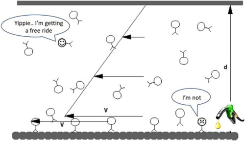
To consider the influence of hydrodynamic forces on the energetics of transport, we begin with a simple two-dimensional model system. We do, however, allow for the fact that motors operate in a bound environment. The system is sketched in Figure 1. Motors move with a velocity v along a track with a bounding wall running parallel to the track a distance d away. The space between is filled with a fluid of viscosity η. Let us assume the bulk concentration of cargo between the track and the fixed ‘top’ of the system is . This concentration is relatively independent of the number density of cargoes attached to the track which has some maximum value (as much as possible attached) that is still small compared to the bulk concentration. We now expect that the movement of the bound cargoes along the track generates a flow field in the fluid (as sketched in Figure 1) and that, since we are in the linear regime, the flow velocity is proportional to the motor velocity v. The flux of unbound cargo taking a ‘free ride’ is then simply proportional to (independent of because the proportion of bound motors is small). Now, the effect of the release mechanism (whereby cargoes also hop off the track) we consider in the following terms. Detaching cargoes reduces to a value below the maximum value while hardly changing , that is the free ride flux is still . Further, we consider the efficiency of the system for a given value of this flux. That is, we examine the amount of energy required to transport material at a given rate. The reason is that this is what a cell must do. It is no use, for example, transporting material very efficiently at a rate so slow, it results in death. The question now is: is there any good energetic reason why motors should detach to reduce the bound motor density?

Figure 1. Some molecular motors do all the work, while others exploit the flow profile to get a free ride.

Experiments measuring the velocity, v, of the motors under an applied external load F show that, to a reasonable approximation, the application of load causes the speed to drop approximately as [15] (1) here the zero load speed and the constant α depend only very weakly on ATP concentration and the viscosity of the fluid [7,16]. Experimental data for Kinesin gives a value for the constant α,  [15], corresponding to a ‘stall force’ (velocity of motor negligible) of . We also have the condition, that the motor does not go into reverse, (2) If we assume a hopping model for the motion of the motor, where it attempts hops with a frequency , and one hop moves it a distance Δ, we then have (3) where is the probability an attempted hop is successful and the probability an attempted hop is unsuccessful. In terms of the model, the effect of an external load is to make some attempted hops unsuccessful. Comparing (1(1) ) and (3(3) ), and assuming all hops are successful if there is no load we have (4) with , being the probability of an unsuccessful attempted hop. One would expect that this is a thermodynamic quantity, so it makes sense that α is independent of the attempted hop frequency.

To proceed we need an estimate for the force acting on the motor and cargo complex. In the experiments[15], the force is an applied external load on a motor in an essentially unbounded fluid. In contrast, here the load is the additional hydrodynamic force exerted on the motor and cargo complex by the bound fluid. Since the cargoes are generally much larger than the motors themselves, this will be dominated by the force on the cargo. Hydrodynamically, one expects that, if the density of motors is high enough, the motor/cargo complexes will act in a similar way to a surface moving with a velocity v subject to a stick boundary condition (the local fluid velocity will match the motor and cargo velocity). This being the case, for the situation sketched in Figure 1, a force density of is required to drive the flow. This force must come from the bound motors so we have, from the continuum result for the force required to drive the flow, an average force acting on each motor, F, (5) This is a simplified view because the actual force experienced by an individual motor will depend on the instantaneous configuration of motors. The simulations that we go on to describe do not make this approximation. Indeed, this is one of the motivations for carrying out the simulations.

If we now substitute this in the equation for the velocity (Equation (4(4) )), we find (6) with restriction (2(2) ) satisfied as long as (7) where .

What can we say about the corresponding energy usage? Experiments have determined that, near to zero load, the rate of consumption of ATP by the molecular motors is consistent with the hydrolysis of a single molecule of ATP per advance of the motor. The corresponding amount of energy consumed per unit length per unit time, E, in the hopping model is therefore (8) where is the energy consumed from one ATP (approximately ). Clearly there is a trade-off between reducing being useful or not useful. On the one hand, there are less motors to drive which saves energy (Equation (8(8) )). On the other hand, to maintain a given velocity the attempted hop frequency will have to increase (Equation (6(6) )), tending to increase energy consumption. Is there an optimal density of bound motors which minimises the energy usage?

If we combine (6(6) ) and (8(8) ), we have (9) Taking the derivative, , we find that for a given velocity the energy consumed does have a minimum at a density (10) (which satisfies the condition, (7(7) ), that we remain below the stall force). We should also note that it is possible that the dependence of the velocity on the force (Equation (1(1) )) is in fact exponential [17]. In this case, our analysis would be an approximation valid for . The final result for the optimal density (Equation (10(10) )) satisfies the condition . In this range experimental results show that a linear relation is still a reasonable approximation [15].

At this point, we can put in some numbers and see if this optimal density is plausible as a mechanism to increase efficiency. The upper limit on , corresponding to the tubule being completely full for the cargo diameter of a, is . We, therefore, have (11) If we substitute the viscosity of water and the experimental value for α, the inverse speed has a value . So, if we measure speeds in units of microns per second (12) Typical values of v are or much less. Even with a high-speed estimate we find that it pays to detach () for . That is, a geometry size of 0.5  for a cargo, which is still pretty small. Of course, for larger values of d, lower values of v or smaller values of a (all plausible), the optimal value of the bound motor density will be much less than the maximum.

This analysis suggests that it is plausible that motors detach from the track to minimise the energy consumed while motors in solution are still transported at the same rate by the flow generated by the bound motors. However, it does consider a rather unrealistic geometry. We now consider a geometry that is more realistic for an axon, for example. Again we assume that the motor and cargo complex acts like a surface with a stick boundary condition. However, we now assume that this surface is a cylindrical surface of radius moving with a velocity in the axial y -direction. The bounding wall is a stationary cylinder with a radius and the two cylinders are coaxial. By considering the transverse momentum flux in the direction of the flow for a hypothetical cylindrical surface located at a distance from the axis, the solution of the linearised Navier–Stokes equation yields a velocity profile of the form (13) with a corresponding force density on the inner cylinder (14) If the density of bound motors per unit area is equal to ρ, and it is the motor cargoes that are exerting the driving force on the fluid, then we can calculate by way of (14(14) ), the force exerted on each motor as being (15) Since the result for the cylindrical symmetry is of the same form as the result for the planar case (Equation (5(5) )) under the substitution (16) we can easily derive the energy usage per unit time per unit length (17) and optimal motor density (18) In terms of the occupation fraction Φ: (19) we find the optimal occupation fraction (20) Note that, due to the logarithmic form of the velocity profile, this result is largely insensitive to the exact location of the outer cylinder . Therefore, that this result may be of value even for geometries where the concept of an ‘outer wall’ is poorly defined, such as irregular environments or even semi-closed geometries.

Let us assume a cargo with radius . In the worst case, the cargo is very close to the track, yielding for the inner radius . For a cargo diameter of we find, taking and as we did in the planar case, that it is energetically favourable to detach for geometries where (21) that is, any geometry where the outer radius is larger than about 4.5 times the inner radius. For a real-world system, this would imply a channel size of about . The width of the channel for which it pays to detach decreases with smaller cargoes, lower velocities and a larger separation between the cargo and the track. In the analysis above we have taken the smallest possible separation (), as well as large estimates for the motor velocity and the cargo size. It is, therefore, likely that detaching motors from the track will prove energetically efficient for smaller channel widths in practice. Axons vary widely in diameter in the range [18], whereas cytoplasmic streaming occurs in cells with sizes of up to millimetres [19]. So the answer we obtain is at least consistent with the real systems in which this type of transport takes place.

3. A simple lattice Boltzmann model for the hydrodynamics of molecular motors

In the previous section, we developed a theoretical model that suggests that it could be energetically favourable for motors to detach from the track because the cargoes in solution take a ‘free ride’ with the flow generated by the bound motors. However, we made an assumption about the form of the hydrodynamic force. In this section, we develop a simple numerical model, using the lattice Boltzmann method to model the fluid [20], to test this assumption.

One drawback of the lattice Boltzmann method is that it is grid based. That is, the flow velocity is only known at discrete points in space. However, if the hydrodynamic coupling between objects in the fluid and the fluid itself is simplified to the level of points that exert friction this restriction can be eased [21,22]. So in the model, the motors and cargo complexes are treated as points that exert friction but are not restricted to discrete positions on the Lattice Boltzmann grid.

To calculate the fluid–motor interaction, at every simulation time-step we find the lattice cell that contains each motor cargo. In the three-dimensional case, we use tri-linear interpolation to determine the fluid density at the position of the motor cargo (22) where are the weight factors for each vertex. For computing the momentum an analogous procedure is used. If we introduce the fractions vector (23) the weight factors are (24) In the two-dimensional case, the former still applies, but only two summations and four factors are actually needed.

Using the fact that , where is the momentum flux, the results of Equation (22(22) ) and the Stokes formula for the drag, we then determine the force that the motor exerts on the fluid (and vice versa) (25) where is the velocity of the motor. This force is then applied to the fluid using the weight factors in Equation (24(24) ).

Essentially, this approach treats the cargoes as points that exert friction on the fluid corresponding to a sphere with radius a. The actual physical size is only accounted for by forbidding bound cargo/motor complexes from having separations of less than . This means that at very small separations the finite size of the cargoes is not correctly accounted for. However, it is not clear that treating the cargoes as actual hard spheres is particularly realistic (or practically possible). Our approach does, however, accurately describe the hydrodynamics on longer length scales (the ‘far field’) so describes collective effects realistically.

One might also ask why, when the motors are actually distributed discretely along the track filament, we do not simply map these points to those of the Lattice Boltzmann grid. The reason is that, as noted above, the cargoes are generally significantly larger than the spacing between discrete binding sites. So doing this would require a proportionately significantly larger system size.

We assume that all the motors are moving at the same velocity and impose a periodic boundary condition in the axial direction. By making a Galilean transformation to the frame of reference of the motors, we can dispense with actually updating the motor positions, as all that it would achieve in the steady state would be to move the entire system through the periodic boundary. While this leaves us with the slightly odd situation of having motors with a finite velocity but no displacement, it makes the simulations vastly easier to implement, test and interpret. To examine the two-dimensional example discussed above we used a planar geometry. A stick boundary condition is imposed on the top of the geometry by using a bounce-back rule [20,23]. The boundary on the track side of the motors is implemented with a slip (bounce-forward) rule. In the three-dimensional case, a cylinder is approximated by rendering cells whose centre falls outside the cylinder volume impenetrable. The interface is realised with a bounce-back rule, which corresponds to a stick boundary condition. A slip boundary condition is implied between the motor/cargo complex and track by allowing the fluid motion to evolve freely. In the two-dimensional case, an interface on the track is required, as that effectively forms one of the boundaries of the system. In the three-dimensional case, the track is completely surrounded by fluid, and no special considerations are needed. One might reasonably ask why we chose a slip condition between the motor-cargo complex and the track. The reasons are as follows. Firstly, it would be pathological to enforce a stick boundary condition because then the motors could not move at all because of lubrication forces. Secondly, the scale of the distance between the cargo and the track is  [14]. One could reasonably expect a continuum hydrodynamic description to break down on this scale. Thirdly, the force that we are considering is actually the additional force due to the confinement of the fluid. There will be some force between the motor and filament even when the fluid is unbounded, but the load force we are considering is the additional force. The slip boundary condition ensures that this is the quantity we calculate because no force arises from the track side.

4. Results

Using the model described above we performed numerical simulations to test the assumptions made in estimating the hydrodynamic force for the planar and cylindrical geometries considered above.

We begin with the planar geometry. For the high-density simulations we use a simulation box of 20 lattice units and 60 lattice units along the track direction. For any given system, there is a minimum value of . So to reach low values, without changing the ratio of a to the bound dimensions, requires that we need to increase the size of the system in the track direction. In this regime, we prefer to fix the number of motors present in the system and adjust the length of the system accordingly. For the minimum density used, , the length of the system grows to 2700 lattice units. We use a value of a=0.243 for the hydrodynamic radius. The distance between the track and the cargo is 0.5 lattice units. In all calculations, we use a motor velocity of .

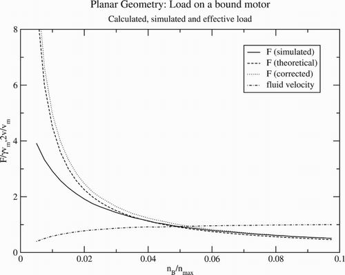
In Figure 2, we show a typical flow profile obtained for a relatively high density of bound motors. As the figure shows, it is well approximated by the constant gradient profile one would expect if the motor-cargo complexes effectively act as a stick boundary. Further this holds to a good approximation at all points along the axial direction, regardless of the configuration of motors. That is, the assumption made in the free ride theory is justified. On the other hand, if the density of motors is sufficiently low this is clearly not the case (see Figure 3). The flow profile is more complex, notably near the motors the streamlines bend in towards the motors. This is a kind of ‘ carburettor’ effect due to the acceleration of the fluid in the vicinity of a motor. In Figure 4, we have plotted the mean flow velocity in the fluid generated by the motor-cargo complexes and the corresponding hydrodynamic force acting on the motors. As the figure shows, the assumption that the force on the bound motors is given by Equation (5(5) ) is justified only while . The same is true for the assumption that the mean flow velocity is proportional to the motor velocity independent of the concentration of bound motors. Below this point the assumption breaks down (Figure 3) and, due to the low concentration of motors, the average fluid velocity progressively drops below the motor velocity. Correspondingly, the hydrodynamic load also drops (the motors are doing less work because they are generating less flow). Since we are operating at a regime where the Navier–Stokes equations that govern the fluid transport are linear, one might suspect that the drop in the force and mean flow velocities are proportionate, that is, (26) This function is also plotted in Figure 4 and as the figure shows, this is the case (to a very good approximation). Consequently, the theory will still correctly predict the load on each molecular motor if we relax the assumption that the flow velocity is constant, but this contradicts our definition of efficiency.

Figure 2. Simulation of the flow near a track in a planar geometry for a relatively high coverage of molecular motors (0.1). The white ‘cargoes’ represent the actual size of the hydrodynamic radius of the particles. The triangle-shaped figure shows the flow profile, which has a constant gradient.

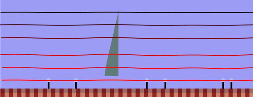
Figure 3. Simulation of the flow near a track in a planar geometry for a relatively low coverage (0.01) of molecular motors. As we can see from the shape of the streamlines, the flow patterns become axially non-uniform and complex.

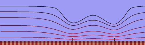
Figure 4. Results from the simulation of the flow near a track in a planar geometry as a function of bound motor coverage.

We now turn to the more realistic case of the coaxial cylindrical geometry. For the high-density simulations, we use a simulation box of 22 lattice units tall, 22 units wide and 60 lattice units long. As we decrease the density, quantisation of the number of motors present becomes an issue. In this regime, again we prefer to fix the number of motors present in the system and adjust the length of the system accordingly. For the minimum density used, the length of the system grows to 2500 lattice units. We use a value of a=0.243 for the hydrodynamic radius. The distance between the track and the cargo is 0.5 lattice unit. In all experiments, we use a motor velocity of .

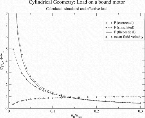
A cross-sectional profile of the flow velocity is shown in Figure 5. Again we see that the velocity profile we expected based on treating the motors as a stick surface is valid at high enough density but at low densities the streamlines near the motor-cargo complexes are distorted and the mean flow velocity decreases relative to the motor velocity. In Figure 6, we again plot the mean flow velocity and hydrodynamic force as a function of bound motor density. The assumption that the action of the motors on the track can be modelled as the solid surface of a cylinder holds up to an area fraction of about . Below that point, as in the planar case, the mean flow velocity and force decrease proportionately. At the cost of introducing an extra parameter , we could re-estimate the optimal motor density based on the simulation results. We do not, however, expect this to qualitatively change the conclusion and the results of the simulations at least confirm that the theory is reasonable as long as the optimal density is not too low.

Figure 5. Flow profile cross section along the radial direction of the coaxial cylinder geometry, for high (0.1) and low (0.01) coverage of bound motors.

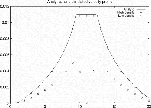
Figure 6. Results for the load on the motors on a track in a coaxial cylindrical geometry as a function of bound motor coverage.

5. Discussion

We have developed a simple theory that suggests that it can be energetically favourable for motors to detach. This is because of the free ride from the fluid flow generated by the bound motors. As the density of bound motors is decreased the free ride flux stays the same while the number of motors running decreases. This saves energy. The density can be decreased to a point where the hydrodynamic force on the motors starts to become significantly higher. Once this point is reached the bound motors start to require more fuel to drag the fluid along. This is energetically unfavourable. A trade-off between these two effects gives an optimal density. The theory predicts an optimal density of bound motors that is plausible (the actual density in vivo is not known). There is nothing adjustable in the theory so it could give any answer for the optimal density from zero to infinity. The fact that it gives something sensible suggests there could well be something in it. There are other explanations, the traffic jam argument for example [24,25]. This notes that if the density of the motors on tubule is too high they get in each other's way and the rate of transport reduces. However, these crowding effects come into play for surface coverage of about , much lower than the optimal values predicted here (at least for relatively low degrees of confinement). There is also the possibility of generating diffusive fluxes from an inhomogeneous distribution of suspended motor-cargo complexes [26,27].

The simple lattice Boltzmann model we developed confirmed the assumption as to the magnitude of the hydrodynamic force acting on the motors at relatively high coverage. It, in principle, also allows us to correct for the fact that the assumption breaks down at low coverage. This does not change the general conclusion from the theory.

The numerical model allows to go further and address more complex geometries and, importantly, transport mechanisms. In particular, for the work reported here the transport is unidirectional. In practice, it is often bidirectional. That is, motors move along different filaments in different directions. One would expect this to significantly change the situation.

One question we have not addressed is how the optimum coverage could be obtained. The degree of coverage is actually determined by the kinetics of attachment and detachment. We do not have the answer to this question but note the following. Because the optimum coverage uses energy at the minimum rate any other coverage will use ATP at a faster rate. If ATP is only being supplied at a given rate, determined by the optimum coverage, any new state can never be a steady state because it would end up running out of ATP. To see if there is a plausible mechanism based on this reasoning requires a more detailed model that takes into account the kinetics of attachment and detachment. At the least we have shown that there is an optimum coverage. Nature may or may not take advantage of it. ATP is generally abundant so maybe it is okay to be wasteful. However, there is considerable interest in constructing microscopic machines using motor proteins [28]. The tubular system we consider, for example, could be realised as a micro pump, if it is the fluid rather than cargoes we are interested in transporting. So even if nature does not make use of the free ride, perhaps when constructing such machines we could?

Disclosure statement

No potential conflict of interest was reported by the authors.

References

- R.D. Vale, Cell 112, 465 (2003). doi: 10.1016/S0092-8674(03)00111-9
- N. Hirokawa, Y. Noda, Y. Tanaka and S. Niwa, Nat. Rev. Mol. Cell Biol. 10, 682 (2003). doi: 10.1038/nrm2774
- A.J. Roberts, T. Kon, P.J. Knight, K. Sutoh and S.A. Burgess, Nat. Rev. Mol. Cell Biol. 14, 713 (2013). doi: 10.1038/nrm3667
- N.L. Badlangana, A. Bhagwandin, K. Fuxe and P.R. Manger, Neuroscience 148, 522 (2007). doi: 10.1016/j.neuroscience.2007.06.005
- A.E. Gioio, J.-T. Chun, M. Crispino, C.P. Capano, A. Giuditta and B.B. Kaplan, J. Neurochem. 63, 13 (1994). doi: 10.1046/j.1471-4159.1994.63010013.x
- G. Pigino, G. Morfini, A. Pelsman, M.P. Mattson, S.T. Brady and J. Busciglio, J. Neurosci 23, 4499 (2003). doi: 10.1523/JNEUROSCI.23-11-04499.2003
- M.J. Schnitzer and S.M. Block, Nature 388, 386 (1997). doi: 10.1038/41111
- C.P. Lowe, Phil. Trans. R. Soc. Lond. B 358, 1543 (2003). doi: 10.1098/rstb.2003.1340
- H. Wang and G. Oster, Europhys. Lett. 57, 134 (2002). doi: 10.1209/epl/i2002-00385-6
- I. Dernyi, M. Bier and R.D. Astumian, Phys. Rev. Lett 83, 903 (1999). doi: 10.1103/PhysRevLett.83.903
- P. Malgaretti, I. Pagonabarraga and D. Frenkel, Phys. Rev. Lett. 109, 168101 (2012). doi: 10.1103/PhysRevLett.109.168101
- A. Esseling-Ozdoba, D. Houtman, A.A van Lammeren, E. Eiser and A.M. Emons, J. Microsci. 231, 274 (2008). doi: 10.1111/j.1365-2818.2008.02033.x
- D. Houtman, I. Pagonabarraga, C.P. Lowe, A. Esseling-Ozdoba, A.M.C. Emons and E. Eiser, Europhys. Lett. 78, 18001 (2007). doi: 10.1209/0295-5075/78/18001
- J. Kerssemakers, J. Howard, H. Hess and S. Diez, PNAS 103, 15812 (2006). doi: 10.1073/pnas.0510400103
- E. Meyhofer and J. Howard, Proc. Natl Acad. Sci 92, 574 (1995). doi: 10.1073/pnas.92.2.574
- K. Visscher, M.J. Schnitzer and S.M. Block, Nature 400, 184 (1999). doi: 10.1038/22146
- O. Camps, Y. Kafri, K.B. Zeldovich, J. Casademunt and J.-F. Joanny, Phys. Rev. Lett. 97, 038101 (2006).
- J.A. Perge, J.E. Niven, E. Mugnaini, V. Balasubramanian and P. Sterling, J. Neurosci. 32, 626 (2012). doi: 10.1523/JNEUROSCI.4254-11.2012
- J. Verchot-Lubicz and R.E. Goldstein, Protoplasma 240, 99 (2010). doi: 10.1007/s00709-009-0088-x
- A.J.C. Ladd, J. Fluid Mech. 271, 285 (1994). doi: 10.1017/S0022112094001771
- P. Ahlrichs and B. Dunweg, Int. J. Mod. Phys. C 9, 1429 (1998). doi: 10.1142/S0129183198001291
- P. Ahlrichs, R. Everaers and B. Dunweg, Phys. Rev. E 64, 040501 (2001). doi: 10.1103/PhysRevE.64.040501
- A.J.C. Ladd, J. Fluid Mech. 271, 311 (1994). doi: 10.1017/S0022112094001783
- R. Lipowsky, S. Klumpp and T.M. Nieuwenhuizen, Phys. Rev. Lett. 87, 108101 (2001). doi: 10.1103/PhysRevLett.87.108101
- D. Chowdhury, A. Schadschneider and K. Nishinari, Phys. Life Rev 2, 318 (2005). doi: 10.1016/j.plrev.2005.09.001
- T.M. Nieuwenhuizen, S. Klumpp and R. Lipowsky, Europhys. Lett. 48, 468 (2002). doi: 10.1209/epl/i2002-00662-4
- T.M. Nieuwenhuizen, S. Klumpp and R. Lipowsky, Phys. Rev. E. 69, 061911 (2004). doi: 10.1103/PhysRevE.69.061911
- J. Clemmens, H. Hess, R. Doot, C.M. Matzke, G.D. Bachand and V. Vogel, Lab Chip 4, 83 (2004). doi: 10.1039/B317059D